The recent star formation in NGC 6822 from HST imaging

Abstract

We present HST WFPC2 and STIS imaging of the low metallicity galaxy NGC 6822, performed as part of a study of the young stellar populations in the galaxies of the Local Group. Eleven WFPC2 pointings, with some overlap, cover two regions, extending over 19 $arcmin^{2}$ and 13 $arcmin^{2}$  respectively, off the galaxy center. The filters used are F170W, F255W, F336W, F439W, and F555W. One 25$\times$25^′′ field observed with STIS’ FUV- and NUV- MAMA, includes Hodge’s OB8 association and the HII region Hubble V, contained in Field 1 of Bianchi et al.: this previous study provides additional WFPC2 four-band photometry.

We derive the physical parameters of the stars in the fields and the extinction by comparing the photometry to grids of model magnitudes. The environments studied in this work include one of the most luminous (in H$\alpha$) HII regions in the Local Group (Hubble V) with a compact star cluster, a typical OB association (OB15), the sparse field population and the outskirts of NGC6822. In the WFPC2 fields, most of the hot massive stars are found in the Hodge OB15 association, at about 5^′ [0.7kpc] East of the galaxy center, extending $\approx 90^{\prime\prime}$ [$\approx 200pc$] in our imaging. The color-magnitude diagram indicates a young age, $\leq$ 10Myrs, for this association, where we measure 70 stars hotter than $\sim$ 16000 K (earlier than mid-B spectral type ) according to their photometric colors. In the compact HII region Hubble V, we measure 80 stars brighter than m_NUV $<$ $22^{m}.5$, most of them have high temperatures. The density [per unit area] of hot massive stars in the core of the OB8 association is higher than in OB15 by a factor of 12, while the total stellar mass formed is similar ($\approx$ 4 or 7 10³ $\cal M_{\odot}$, when extrapolated to a mass range of 1-100$\cal M_{\odot}$  or 0.1-100$\cal M_{\odot}$respectively). In both OB15 and OB8 massive star candidates are found. In the general field outside of the OB15 association, we find few hot massive stars (0.7/arcmin²) and several A-type supergiants. No massive star candidates are found in the WFPC2 fields outside the main galaxy body ($\approx$ 10.5-14.5^′ [1.5-2.kpc] from the galaxy center), where the population is dominated by foreground stars, at least down to $V\sim 22$. At fainter magnitudes, we measure in these outer fields a significantly larger number of stars than the model for MW foreground objects would predict. The average extinction is found to vary among the three environments studied: $E(B-V)$= 0.22 in the outer regions, $E(B-V)$= 0.27 in the fields East of the galaxy main bar, and $E(B-V)$= 0.40 in the HII region Hubble V.

A quantitative discussion of the applicability of the reddening-free-index method for photometric determination of stellar parameters is provided for the filters used in this work, based on our grids of stellar models.

1 Introduction

The massive star populations of nearby galaxies are a subject of great interest, due to the impact that massive stars have on the galaxies’ properties and evolution. Massive stars, in their short lifetime, drive the chemical and dynamical evolution of the parent galaxies and trace the star–formation activity. The most luminous, most massive stars provide information on the Initial Mass Function (IMF) and its properties. The study of the IMF in different environments gives us a way to determine its dependence on parameters such as metallicity and star–formation rate. The galaxies of the Local Group provide an excellent opportunity to investigate the modalities of star formation through the resolved studies of their stellar populations, because they are close enough so that individual stars can be accurately measured, and all the stars are at approximately the same, known distance thus their absolute luminosity can be derived. With its high resolving power, and wide range of filters including UV wavelengths, the Hubble Space Telescope (HST) is the most suitable instrument for studying young stellar populations in the Local Group galaxies. In a global context, studies of resolved local starbursts provide a key to understand distant star-forming galaxies, for which only integrated properties can be measured. Resolved studies of the stellar content, extinction and global parameters of nearby starburst regions in different environments provide a calibration to interpret integrated studies of unresolved starbursts in distant galaxies.

NGC 6822 is an irregular dwarf galaxy, a member of the Local Group. The angular size of the galaxy at optical wavelengths is $6^{\prime}\times 11^{\prime}$ and its distance is estimated to be 500 kpc (McGonegal at al. 1983).

The old and intermediate stellar populations of NGC 6822 have been studied by Gallart et al. (1996) on a central 11.2^′ $\times$ 10.4^′ area, and by Wyder (2003) in four HST-WFPC2 fields, from V and I band photometry. Both studies infer from the CMD that the star formation began 12-15Gyr ago or more recently, depending on the initial metallicity assumed, and proceeded more or less uniformly until about 600Myr ago. The young stellar population of NGC 6822, and its recent star formation history, has also been the subject of previous photometric studies. The first galaxy–wide photographic UBV photometry of NGC 6822 was published by Kayser (1967), followed by a photographic and photoelectric study by Hodge (1977), who catalogued sixteen OB associations. Massey et al. (1995) ground-based photometric study found that O-type stars are present in several of the OB associations, but that NGC 6822 is relatively poor in very massive stars compared to M31, M33 and the Magellanic Clouds; the reddening varies from $E(B-V)$=0.26 on the periphery to 0.45 near the central regions, with an average ratio $E(U-B)/E(B-V)$ of $0.74\pm 0.07$. Bianchi at al. (2001a) presented ground–based UBV CCD photometry covering the whole body of the galaxy and HST Wide Field Planetary Camera 2 (WFPC2) four band photometry in two regions containing very rich and crowded OB associations. They found populations younger than 10 Myr in four of the OB associations included in their study, and in particular very young stellar populations (few Myr) in the star–forming HII regions Hubble V and Hubble X (Hubble 1925). The outer parts of the galaxy are much less studied. No young stellar population was found in the two outer regions of NGC 6822 analyzed by Hutchings, Cavanagh, & Bianchi (1999).

The search for young stars in different galaxy environments presented in this paper covers larger regions than previous HST studies, with deeper exposures, and has the advantages of the HST wide wavelength coverage (extending to the UV), and higher spatial resolution, compared to the ground-based UBV data. The UV bands (WFPC2 F170W and F255W, Space Telescope Imaging Spectrograph (STIS) MAMA-FUV and MAMA-NUV) in addition to the U, B, V bands, allow us to identify the most massive, luminous stars. In fact, due to their high effective temperatures, the earliest spectral types cannot be differenciated from optical colors (see e.g. the discussion in Massey (1998a) and Bianchi & Tolea, 2006, in preparation).

The observations and data reduction are described in section 2, the photometry measurements and the characteristics of the stellar populations are presented in section 3, the results are discussed in section 4, and summarized in Section 5.

2 Observations and Data Reduction. Photometry.

Hubble Space Telescope (HST) imaging of different regions in NGC 6822 were obtained between 6/16/2000 and 5/24/2002 as part of the program GO 8675 (P.I. L. Bianchi) to study the massive star content of this galaxy, with the Wide Field and Planetary Camera 2 (WFPC2) and the Space Telescope Imaging Spectrograph (STIS) imagers. The WFPC2 images were taken in parallel mode. We discuss the reduction and analysis procedures separately for the two sets of data. The photometry and the derived parameters for the sample stars are given in Table 3 (printed for the hottest stars subsample, in electronic form for the entire sample), and 4 (STIS data).

2.1 WFPC2 imaging

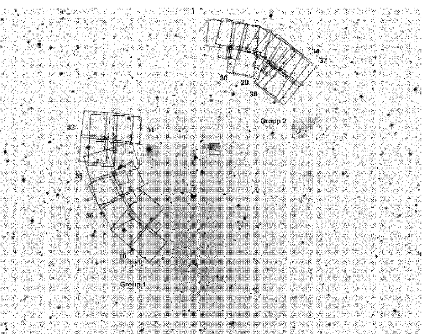
Figure 1: Ground-based V-band image ($\approx$ 21^′ $\times$ 16 ^′ ) of NGC 6822 with outlined WFPC2 and STIS fields. North is up, East is to the left. The small square between the two WFPC2 groups indicates the STIS field.

A total of 110 images in 11 different fields were obtained with WFPC2 on-board HST. The instrument consists of four $800\times 800$ CCD chips with angular resolution of $0\arcsec.046\,pix^{-1}$ [0.11pc at the distance of 500 kpc to NGC6822] for the Planetary Camera (PC) and $0\arcsec.099\,pix^{-1}$ [0.24pc] for the Wide Field chips (WF2, WF3 and WF4). In most of the fields imaging was taken with five WFPC2 broad – band filters: F170W, F255W, F336W, F439W and F555W. Table 1 lists the field positions, the filters used and the corresponding exposure times. The fields are partially overlapping, and are grouped in two areas, East and North-West the main body of the galaxy. The East group (Group 1), covers about 19 $arcmin^{2}$[$\approx$ 402kpc²] , and the N-W group (Group 2), covers about 13 $arcmin^{2}$[$\approx$ 275 kpc²]. The positions of the fields are shown in Figure 1.

The images processed with the Post Observation Data Processing System (PODS) pipeline for bias removal and flat fielding were downloaded from the MAST archive. In order to reject the cosmic rays, images taken with the same pointing and filter were combined using the IRAF task CRREJ. This task combines multiple exposures at the same pointing and rejects the high counts that occur in only one of the frames. It was possible to apply this procedure to all the fields, because we have at least two images per filter for each pointing. The Source Extractor code (Bertin and Arnouts 1996) was then used to detect the star-like objects exceeding the local background by more than $3.5~{}\sigma$ in the F555W images. Then aperture photometry was performed, using the same positions in all the filters. Slight recentering (less than 2 pixels) from the F555W position was needed to optimize centering of the objects from filter to filter. We performed the photometry with the PHOT task in the DAOPHOT/IRAF package, using the source list and positions from Source Extractor. The aperture chosen for both PC and WF chips was 3 pixels, and the sky was measured in an annulus with inner and outer radii of 5 and 8 pixels respectively. Aperture corrections to 0″.5 aperture were measured using isolated stars separately for the different chips and filters. Aperture photometry was chosen over psf photometry to ensure a uniform procedure among our fields, and consistent with previous works. Crowding effects are negligible in our fields. The WFPC2 fields in particular contain fairly sparse populations (the most crowded region is shown in Fig.6), and the only crowded region, Hubble V, was observed with STIS at UV wavelengths, where crowding is much less than at optical wavelengths. The flux calibration was performed following Holtzman et al. (1995a,b) with the refinements of Dolphin (2000), and included the following steps: (i) Distortion Correction: geometric distortion affects the integration in the photometric aperture. To account for this effect our images were multiplied by the correction image provided by Holtzman et al. (1995b). (ii) Correction for Contamination: due to contaminants buildup on the cold CCD plate the UV throughput decreases. The photometric correction to be applied depends on the time elapsed since the last decontamination procedure. Decontamination correction coefficients were taken from McMaster & Whitmore (2002). (iii) Charge Transfer Efficiency (CTE) correction: the formula of Dolphin (2000) was applied.

The magnitudes were then transformed in the HST VEGAMAG photometric system by applying the zero points as follows: for F336W, F439W and F555W, we used the zero points from Dolphin’s (2002) web site, which are relative to a 0″.5 aperture. The zero points for F170W and F255W were taken from the HST Data Handbook for WFPC2 with a $0^{m}.1$ correction for the transition from infinite to 0″.5 aperture. For our analysis we used the VEGAMAG WFPC2 photometric system, but in Table 3 (the hottest stars) the F336W, F439W and F555W magnitudes are also transformed to the Johnson’s UBV system to allow comparisons with other works. The error vs magnitude plots of a typical field (FIELD 10) for all the filters used are shown in Figure 2. Such diagrams are used to estimate the magnitude limits of our sample after we impose error cuts for the analysis described in Section 3.

The overlapping fields were processed separately and photometry was performed in each field independently. The measured magnitudes of stars included in several fields are consistent within the errors. The magnitude given in the final catalog is an error weighted average of all the measurements for the same star. The formula used is $\overline{m}=\frac{\sum_{i=1}^{n}\frac{m_{i}}{\Delta m_{i}^{2}}}{\sum_{i=1}^{n}\frac{1}{\Delta m_{i}^{2}}}$, where n is the number of overlapping fields in which the star is present. The corresponding error is calculated as: $\overline{\Delta m}=(\sum_{i=1}^{n}\frac{1}{\Delta m_{i}^{2}})^{-1/2}$

The deepest observations are in the F555W band, where 18244 stars are detected (above 3.5$\sigma$); 12423 (70%) of them have photometric accuracy better than $0^{m}.2$. The number of stars with errors smaller than $0^{m}.2$ in the F439W filter is 1757 and in F336W the number of stars with accuracy better than $0^{m}.2$ is only 535 (2.7% of the stars detected in F555W). Fewer stars are detectable in F170 and F255 with accuracy better than $0^{m}.2$. See Table 2 for details on errors and magnitude limits in the different filters.

2.2 STIS imaging

Four overlapping STIS images were taken with the 25MAMA aperture using the FUV-MAMA and NUV-MAMA photon counting detectors. All the images are centered at $RA\approx 19\,44\,52.2$ and $Dec\approx-14\,43\,14.5$ and cover a $25^{\prime\prime}\times 25^{\prime\prime}$ [60 $\times$ 60 pc] field of view. The size of the detectors is $1024\times 1024\,pixels$, and the resolution is $0^{\prime\prime}.024pixel^{-1}$ [0.06 pc], providing the highest resolution view of the compact HII region Hubble V to date. Details about the images are listed in Table 1. The STIS data were downloaded after being calibrated through the STScI calstis pipeline. Aperture photometry (5 pixels) was performed using the PHOT task in the DAOPHOT/IRAF package. The aperture corrections were measured from 20.8 pixel aperture (corresponding to $0^{\prime\prime}.5$) photometry of selected stars. The measured magnitudes were converted to the HST VEGAMAG system. There are 80 stars detected in both NUV and FUV. The magnitude - error diagram is shown in Figure 3, and the magnitude limits are listed in Table  2. Our entire STIS field is included in WFPC2 Field 1 of Bianchi et al. (2001a). This previous work provides photometry in four WFPC2 filters, F555W, F439W, F336W and F255W, that will be combined with the UV STIS photometry in the analysis described in the next section. The STIS images contain the OB8 association (Hodge 1977) embedded in the HII region Hubble V. The STIS imaging provides a gain of over 2 magnitudes in NUV with respect to the earlier WFPC2 data, and the first observations of this region in the FUV. We have six band photometry (four bands from Bianchi et al. 2001a WFPC2 photometry and two from our STIS photometry) for 72 out of the 80 stars detected in our STIS imaging.

3 Analysis. The Stellar Populations

In this section we analyze the multi-band photometry of individual stars and derive their physical parameters by comparison with model colors. Two methods are used, and the results are compared. For the stars with good photometric measurements in all the filters, we fit all the observed colors with model colors, to which various reddening amounts are applied, and derive simultaneously stellar $T_{\rm eff}$  and interstellar extinction. For the stars not detected in the UV filters, or with large uncertainties in the UV-band measurements, we use a method similar to the traditional “reddening-free” Q index.

3.1 The WFPC2 photometry. Foreground contamination

The observational color – magnitude diagrams in the F336W, F439W and F555W filters are shown in Figure 4, for all stars in the Group 1 fields (open circles) and in the Group 2 fields (filled circles). The dashed lines indicate the magnitude limits of the “restricted sample” analysed in the following sections.

As described in earlier studies a “blue plume” is present, at $(B-V)\approx 0$ (see e.g. Bianchi et al. 2001a) indicating H-burning massive stars, especially prominent in the Group 1 population. There are a few blue stars in the outer parts of NGC 6822 (Group 2 fields). Most of the blue stars in our sample are found in the Group 1 fields which are closer to the main body of the galaxy. The majority of the blue stars is located in the WF3 chip of Field 36, shown in Figure 6. This field contains most of the association OB15 identified by Hodge (1977). There are 47 blue stars with good photometry in all the five filters, 46 of them in the “Group 1” fields and only one in the “Group 2” fields. Their photometry is given in Table  3.

The majority of red and intermediate color stars in our sample is expected to be foreground contamination at the latitude of NGC 6822. The model of Ratnatunga & Bachall (1985) predicts most of the foreground stars in the direction of NGC 6822 with observed magnitudes $17\leq\mbox{$m_{V}$}\leq 22$ to have $0.8\leq(B-V)\leq 1.3$, which is the area of the HR diagram where most of the stars from the “Group 2” fields are found. There is excellent agreement between the expected number of foreground stars in a given color and visual magnitude range, and the number of Group 2 stars with the same colors and magnitudes, for the brighter magnitudes, but at fainter magnitudes the number of stars measured exceeds the number of predicted foreground stars (Figure 5). The number of foreground stars given in the figure is calculated from the model of Ratnatunga & Bachall (1985) for an area $13\mbox{$arcmin^{2}$}$ (as covered by our Group 2 fields), the number of stars detected in each bin is also reported. For magnitudes above the limits of our “restricted sample” (next section) there is good agreement, suggesting that most stars in “Group 2” are foreground, therefore we can use the “Group 2” sample to estimate the foreground contamination in the “Group 1” sample, above $V\approx 22$. At fainter magnitudes, we detect significantly more objects than predicted by the Ratnatunga & Bachall (1985) model. However, these authors warn that for $20>|b|>10$ or $V>22$ their model should be used with caution because these regions are outside the Galactic latitudes or apparent magnitudes tested. We cannot establish, with our present sample, whether the excess of faint stars (up to 7 times more stars detected than predicted for (B-V)$<$0.8 and $21>V>23$) is due to an old population in the outskirts of NGC 6822, or if the model of Ratnatunga & Bachall (1985) needs to be significantly revised in this magnitude range. The question could be clarified by deep imaging with a ground-based telescope.

Using the CMD of the Group 2 sample to estimate the foreground contamination of the Group 1 sample, we find that the majority ($\approx 70\%$) of the intermediate color stars ($0.8\leq(B-V)\leq 1.3$) are foreground objects. The fraction drops to $\approx 30\%$ for stars with bluer color ($0.3\leq(B-V)\leq 0.8$), and is negligible at $B-V\approx 0$. We conclude that foreground stars are a significant contamination in the red part of the CMD (both from the Ratnatunga & Bachall model and by using our Group 2 fields as a proxy for the foreground stars estimate) while they don’t affect the estimate of the hot massive stars ($(B-V)\approx 0$) content.

3.2 Derivation of stellar parameters

Here we use the observed photometry to determine the stellar physical parameters. In the first method, known as the “Q-method”, we construct reddening free indexes (Q), using different combinations of two colors to determine the amount of reddening and the stellar temperature concurrently. This method is applicable to all stars that have good measurements in at least three photometric bands. In the second method we determine the values of $E(B-V)$  and $T_{\rm eff}$  using all available bands by simultaneous fitting of the observed colors to synthetic colors using $\chi^{2}$ minimization. For this purpose we used both a modified version of the Bianchi et al. (2001a), Romaniello (1998) code, and the CHORIZOS code by Maíz-Apellaniz (2004). Both codes give consistent results. This method is applicable to the stars with good photometry in four or more bands.

To describe the analysis with the reddening-free index method, we first consider photometry in the F336W, F439W, and F555W filters, since our data reach fainter magnitudes in these bands (figure 2). We limit the analysis to stars with photometric errors of 0.05, 0.08 and 0.10 mag in F555W, F439W and F336W respectively (“restricted sample”). The error on the reddening-free index, and hence on the derived parameters, is a combination of the errors in the three bands. We applied a progressively less stringent error cut from the V-band to the U-band measurements, in order to approximately match the depth of the sample in these three bands for the “blue plume”, and still have an overall good accuracy of the Q-index. The blue plume has average colors of (m₄₃₉ - m₅₅₅) $\approx$ 0.2 and (m₃₃₆ - m₄₃₉) $\approx$ -1.2, therefore the same “depth” of the sample is reached for m₃₃₆ $\approx$ m₄₃₉ - 1.2 $\sim$ m₅₅₅ - 1. Our chosen error cut of 0.1 mag for the m₃₃₆ magnitudes, limits the m₃₃₆ measurements to $\sim$ 21.5 mag (figure 2). The corresponding errors limits in m₄₃₉ and m₅₅₅ are 0.08 and 0.05 mag for our “restricted sample”. These error limits combined translate in a maximum uncertainty for reddening-free index of Q_err$<$ 0.16, which propagates into errors on the derived parameters according to the parameters regime, as can be seen in Figure 7. The restricted sample defined above is hence limited to m₅₅₅ $\sim$ 22.5 mag, and the number of objects to 230. For red supergiants, having (m₄₃₉ - m₅₅₅) $\approx$ 1. and (m₃₃₆ - m₄₃₉) $\approx$ 0.–0.5, the limit of our restricted sample becomes m₅₅₅ $\sim$ 20.5–21.0 mag, basically driven by the U-band error cut of 0.1 mag. We also consider a less restrictive sample (“wider sample”), with error limits of 0.17, 0.11, and 0.07 mag in m₃₃₆, m₄₃₉ and m₅₅₅ respectively (Q_err$<$0.24), which increases the number of objects by 130 stars, and extends the limit to m₅₅₅ $\sim$ 23 mag. The total number of objects in the “wider sample” is therefore 360; values of $T_{\rm eff}$  and $E(B-V)$  from the analysis described below are given in Table 3 (electronic version) for 345 stars of this sample; the remaining 15 objects have colors in the range where the Q-method is not applicable (Q is not reddening-free), and are probably foreground cool stars. Table 2 gives the number of objects in each filter within given error limits.

The “reddening free” Q index is a combination of two different colors (usually from three bands) with the ratio of the two color-excesses, so that its value does not depend on the reddening. The classical Q-index is constructed with magnitudes in U, B and V (e.g. Massey 1998a):

$$Q_{UBV}=(U-B)-\frac{E(U-B)}{E(B-V)}(B-V)=$$

$$=(U-B)_{0}+E(U-B)-\frac{E(U-B)}{E(B-V)}[(B-V)_{0}+E(B-V)]=$$

$$=(U-B)_{0}-\frac{E(U-B)}{E(B-V)}(B-V)_{0}=Q_{UBV0},$$

where the subscript ₀ indicates intrinsic colors. A similar index can be constructed for any combination of at least three filters. The observed value of $Q$ is equal to the intrinsic one, hence it provides a reddening independent direct measurement of $T_{\rm eff}$, to the extent that the ratio $C=\frac{E(U-B)}{E(B-V)}$ is actually constant. This is a good approximation for low values of $E(B-V)$. If we were using monochromatic fluxes, $C$ would be constant for any amount of reddening, and would only depend on the type of extinction, i.e. on the extinction curve adopted. In practice, when we use broad band filters, because both $T_{\rm eff}$  and reddening variations change the slope of the spectrum within the band, $C$ is constant only within limited ranges of $E(B-V)$  and $T_{\rm eff}$  (see Bianchi & Tolea 2006 for further discussion).

We constructed Q indexes (as a function of stellar parameters) in the HST filter system using a grid of synthetic colors, obtained by applying the transmission curves of the WFPC2 filters to Kurucz synthetic stellar spectra models of Lejeune et al. (1997) and Bianchi et al. (in preparation). Our model colors cover a large range in stellar parameters $T_{\rm eff}$ and log(g), for different metallicities. The effects of differing amounts and types of extinction are applied to the model spectra, and synthetic colors are computed applying the filter curves to the reddened models. Therefore, our grids of model colors allow us to also derive the value of C for various types of reddening, and to verify within what limits it remains actually constant. We initially adopt MW type extinction ($R_{V}=3.1$) assuming that in our sample most of the extinction is due to Milky Way foreground dust, which is confirmed by our results. The MW reddening law ($R_{V}=3.1$) was also found appropriate for NGC 6822 by Massey et al. (1995). From our model colors, we found $C_{F336W,F439W,F555W}$ to be constant in the temperature range $\mbox{$T_{\rm eff}$}\in[8000,50000]$ and $E(B-V)$$<$ 0.7], with a value of $C_{F336W,F439W,F555W}$ =0.96. We use the $Q_{F336W,F439W,F555W}$ index to derive the extinction and the stellar temperatures in these intervals. We can also use $Q_{F336W,F439W,F555W}$ for the stars in the range $\mbox{$T_{\rm eff}$}\in[5000,8000]$ and $E(B-V)$$<$ 0.7], with $C_{F336W,F439W,F555W}$=0.90.

Because a higher reddening applied to a hot star spectrum can mimic a less reddened cooler spectrum, in certain parameter ranges the solution [$T_{\rm eff}$, $E(B-V)$] is not unique, as can be seen from Figure 7. Since the Q index is reddening independent (within the applicable range), on the Color – Q diagram the reddening only displaces the points in color (along the x-axis in figure 7). The difference in color between the observed points and the model colors (corresponding to the intrinsic colors) provides an estimate of the extinction, while the value of Q provides $T_{\rm eff}$. In the ranges where, for a given observed color and Q, the intrinsic color has more than one possible value ( $Q_{F336W,F439W,F555W}\in[-0.7,-0.2]$, (m₄₃₉ - m₅₅₅) $>$ 0.2 for solar metallicity, see Figure 7) different solutions for [ $T_{\rm eff}$, $E(B-V)$] exist.

In the upper panel of Figure 7 we plot the synthetic $Q_{F336W,F439W,F555W}$ index vs the color $\mbox{$m_{439}$}-\mbox{$m_{555}$}$. The observed values are shown as dots for our “restricted” sample (stars with error in Q better than 0.16), and with crosses for the “wider” sample (0.24$>Q_{err}>$0.16). The solid lines represent model colors for main sequence stars (thick: solar metallicity, thin: Z=0.002). The model curves show that: for $Q_{F336W,F439W,F555W}$ $\lesssim$ - 0.7 (the exact value slightly depending on metallicity) there is only one solution; for more positive values of $Q_{F336W,F439W,F555W}$ there are the following possibilities: when $(\mbox{$m_{439}$}-\mbox{$m_{555}$})\leq 0.1$ there is a unique solution for [$E(B-V)$,$T_{\rm eff}$], for stars with $0.1<(\mbox{$m_{439}$}-\mbox{$m_{555}$})<0.6$ there are two possible solutions, and for $(\mbox{$m_{439}$}-\mbox{$m_{555}$})>0.6$, there are three possible solutions. In the case of this study, however, we notice that when there are more than one possible solution, the lowest value of $E(B-V)$  is similar to the average $E(B-V)$  in the field. The values of $E(B-V)$  from the other possible solutions significantly exceed any value of $E(B-V)$  determined in these fields for the stars with a unique solution, and exceed by $\sim$ 0.8 mag the average $E(B-V)$  determined in the galaxy by this and previous works. This difference can be appreciated at a glance from figure 7. Therefore we choose the solution [$E(B-V)$, $T_{\rm eff}$ ] with the lowest extinction value, assuming that there is no reason for the extinction to vary extremely in such sparse fields. For the same reason, for those stars that have $(\mbox{$m_{439}$}-\mbox{$m_{555}$})>0.5$ and formally a unique solution from the Q- diagram implying $E(B-V)$$>$ 0.5, we adopted instead the average value of $E(B-V)$= 0.27 (as determined from the “restricted sample” in the field population outside of OB15) for those stars in the “Group 1” fields, and $E(B-V)$= 0.2 for those located in the “Group 2” fields. These objects are seen as a small “plume” above the model-Q curves for red stars in figure 7, and are indentified with flags “c” and “d” respectively in the electronic version of Table 3. Theoretically, they could be hot stars with very high extinction, but the majority is likely foreground stars.

An interesting feature of the color $-$ Q diagram is the separation of the model color curves for different gravities. Main sequence (solid lines), and supergiants (dashed lines) are plotted in the $T_{\rm eff}$  range [50000, 4000] in Fig. 7. The curves separate for $T_{\rm eff}$$\lesssim$ 10,000 K ($Q>-0.2$). A group of $\approx$ 25 stars with high values of Q can be classified as supergiants, based on the photometry, indicating that these cooler objects belong to NGC 6822 and are not foreground stars. They are found in the “Group 1” fields, (4 in the area of OB15) and only 1 or 2 are found in the “Group 2” fields.

We have also calculated $Q_{F336W,F439W,F555W}$ using low metallicity models (Z=0.002; thin lines in Fig. 7 upper panel) in order to check how metallicity affects the color – Q diagram. The solutions for hot stars (down to 10000K) do not differ significantly with metallicity but for low temperature stars the results for $E(B-V)$  and $T_{\rm eff}$  depend on metallicity. This paper is focussed on the hot massive stellar population of NGC6822, so the choice of metallicity does not affect our results.

For stars detected also in the UV, we constructed additional Q indexes including the F170W magnitude, which provides a more sensitive measurement of the high temperatures and especially of the extinction. As shown in the bottom panel of Figure 7, $Q_{F170W,F439W,F555W}$ spans over 2 mag in the $T_{\rm eff}$  range 10000-35000 K, compared to the $\sim$1 mag variation of Q_{F336W,F439W,F555W}. However, the larger uncertainties in the UV photometry, due to the lower sensitivity of the CCD at UV wavelengths, limit the advantage of these broader wavelength coverage to the hottest objects. We found, from our model colors, $C_{F170W,F439W,F555W}$=4.15, approximately constant for $\mbox{$T_{\rm eff}$}\in[11000,50000]$ and $\mbox{$E(B-V)$}<$ 0.7. The model values of $Q_{F170W,F439W,F555W}$ for low gravity stars again separate from the dwarfs for temperatures between 10000K and 8000K. This part of the diagram is not shown since only the hottest stars in our sample are detected in F170W. The analysis using 5 band photometry is restricted to objects with photometric accuracy in F170W and F255W better than $0^{m}.2$. There are 47 such stars in the WFPC2 sample. All of the stars with good photometry in five bands lay in the unique-solution part of the Color – Q diagrams, and the values of $E(B-V)$  and $T_{\rm eff}$  obtained from different Q indexes are consistent within the errors.

For our restricted sample $E(B-V)$  varies between 0.17 and 0.37, with a mean value of $E(B-V)$  of 0.27 which is in agreement with the estimate of Massey et al. (1995) for the outer parts of NGC 6822.

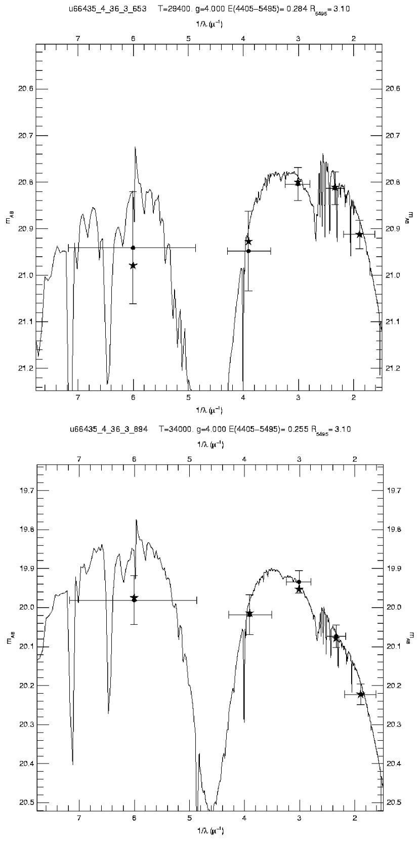
Figure 8: Two examples of $\chi^{2}$ fits obtained with the CHORIZOS code. The crosses are the observed magnitudes with their errors, the stars are the synthetic magnitudes with the width of the filters. The model spectrum from which the synthetic magnitudes are generated is also shown. The lines appear very strong in the spectrum because of the flux scale in magnitudes.

In the second method we derive the values of extinction and stellar temperature by simultaneous $\chi^{2}$ minimization fitting of all the observed colors with the same library of model colors. The advantage of this method is the use of all the available photometric information simultaneously, each magnitude being weighted according to its uncertainty. We used the CHORIZOS code by Maíz-Apellaniz (2004), as well as a code developed by us (based on the method by Romaniello 1998) and find consistent results. We obtain a good fit with $\chi^{2}\in[0.6,5.5]$ for approximately $60\%$ of the stars with five band photometry. Two examples of good fits are shown in Fig. 8. The model spectrum that best fits the observed colors is shown along with the model magnitudes and the observed magnitudes with their errors. The derived $T_{\rm eff}$  and $E(B-V)$  correlate well with the values obtained from the Q – method within the errors, although there is a slight trend of higher extinction values, and consequently $T_{\rm eff}$, from the $\chi^{2}$ fit.

In both the reddening-free and the $\chi$² fitting method we used MW-type extinction with R_V=3.1 and also tried UV-steeper extinction laws, such as LMC-type extinction. We found the MW-type extinction to provide better match to the observed photometry, consistent with the result that most of the extinction is due to foreground MW dust. In order to construct physical HR diagrams (next section), for the stars with five band photometry we adopt the values of $T_{\rm eff}$  and reddening from the $\chi^{2}$ fit (given in the printed version of Table 3) and for the stars with three good measurements the values from the Q – method. Stars with B and V measurements having errors better than 0.2 mag, but errors larger than our “wider sample” limits in other bands, are also included the end of Table 3 (electronic version).

3.3 STIS photometry

Most of the UV sources (72 out of 80) in the STIS imaging of OB 8 have measured counterparts in the WFPC2 photometry of Bianchi et al. (2001a) that provides additional measurements in four bands: F255W, F336W, F439W, and F555W. We derived temperatures and $E(B-V)$  by comparing the photometry to the model colors as described in the previous section, using $\chi^{2}$ fitting.

The additional STIS FUV band gives us the opportunity to refine the determination of extinction and temperature with respect to our previous work. The errors in the WFPC2 imaging of Bianchi et al. (2001a) in the F255W and F336W filters are larger than 0.2 mag for more than one third of the sample, and our new STIS UV photometry with relatively small errors significantly improves the determination of the stellar parameters. The stellar temperatures determined from the $\chi^{2}$ fit including UV bands tend to be higher than the previous results. The HR diagram of the Hubble V region is shown in fig.  10 with filled circles. The results from the photometry of Bianchi et al. (2001a) are shown with crosses for comparison. The photometric measurements and derived stellar parameters, as well as the identification with the sources from Bianchi et al. (2001) are listed in Table 4. The coordinates are from the STIS images, however we applied a constant shift of $+0.684^{\prime\prime}$ and $-0.54^{\prime\prime}$ in R.A., and $-0.684^{\prime\prime}$ and $-0.72^{\prime\prime}$ in declination, for fields o66410 and o66420 respectively, in order to register the astrometry to the WFPC2 coordinates of Bianchi et al. (2001). After the shift, positions for matched stars coincide within 0.2” arcseconds.

4 Results and Discussion

Absolute magnitudes for our sample were calculated using the reddening derived in the previous section and a distance modulus of DM=23.47 (McGonegal at al. 1983). In Figure 9 the Color–Magnitude diagram for stars in the Group 1 fields is shown with superimposed theoretical isochrones for Z=0.004 from Girardi et al. (2002) and Bertelli et al. (1994). Isochrones for solar metallicity do not fit as well the observations. The majority of the Group 1 stars with five band photometry (34 stars, or 74%) are in the association OB15 (Hodge 1977) centered at $\alpha=19^{h}\,45^{m}\,14^{s}$ , $\delta=-14^{\circ}\,45^{m}\,7^{s}$, with an angular size of $\approx 90^{\prime\prime}$ ($\approx 200pc$ linear size), and a distance from the center of the galaxy of $\approx 5^{\prime}$ or 730 pc. The main part of the association is included in the WF3 chip of Field 36 shown in Fig. 6. For these stars we estimated $T_{\rm eff}$$>$ 20,000 K (spectral type earlier than B2). Their “scale distance”, defined as the largest distance between two close neighbors in the group (see Battinelli 1991 and Ivanov 1996) is $d_{S}=26\arcsec\,(46pc)$, and the mean distance between close neighbors is $d_{M}=5\arcsec\,(13pc)$, with $\sigma=4.5\arcsec\,(11.4pc)$. If we add fainter hot star candidates that have photometry only in three bands, using the $(\mbox{$m_{336}$}-\mbox{$m_{439}$})_{o}<-1$ and $(\mbox{$m_{439}$}-\mbox{$m_{555}$})_{o}<0.0$ criteria to select stars hotter than 16,000 K (i.e. earlier than sp.type $\sim$ B5 V), we find 35 additional stars in OB 15 (down to magnitude V_o= 22.2 (V$\approx$ 23.0, M_V=-1.27) and the association properties become $d_{S}=13\arcsec\,(32pc)$ and $d_{M}=4\arcsec\,(10pc)$ with $\sigma=3\arcsec\,(8pc)$. The total number of stars with estimated $T_{\rm eff}$$>$ 16,000 K in OB 15, is therefore about 70. The expected foreground contamination is negligible for the hot star sample (Section 3.1), so we assume all of the observed massive stars to be members of the OB association. The HR diagram indicates the stellar population in OB15 to be younger than 10 Myr.

Our data, geared towards the characterization of the young massive stars, do not provide conclusive information on the number of red supergiants. In fact, the U-band filter drives the magnitude limit in our “restricted sample” to very bright limits for cool stars ($m_{555}$ $\approx$ 20.5, or $(m_{555})_{o}$ =19.7/19.3 in OB8 and OB15 respectively). If we consider the (B-V) color only, we can reach fainter magnitudes (see figure 4) but we have no way to separate the foreground (MW halo) dwarfs from the NGC 6822 supergiants, whose apparent magnitudes are in the same range (e.g. Massey 1998c, Bianchi et al. 2001b). The number of red foreground stars ($(B-V)$ $>$ 1.3 ) expected from the model of Ratnatunga & Bachall (1985) is 0.35 per square arcmin down to V=19 and 1.5 per square arcmin between V=19 and 21. Therefore, we expect 24 and 35 red foreground stars brighter than V=21 in our Group 2 and Group 1 samples respectively. The number of stars with measured photometry $(B-V)$ $>$ 1.3, V $<$ 21, is 14 and 32 respectively in the Group 2 and Group 1 samples. Considering the effects of small number statistics, no detection of red supergiants can be claimed without spectroscopic follow-up, which we plan to pursue. A better estimate of the evolved stellar population in this region can be obtained from the red supergiants survey of Massey (1998c). This survey is complete (photometrically) to V=20.5. The OB15 association is contained in Massey’s N6822-C field. There is only one star (NGC 6822c-438) from the Massey (1998c) catalog inside the OB15 area, and it is classified by the author as a foreground object. The 4 closest neighbors are also classified as foreground stars, so we can conclude that there are no red supergiants in the region of OB15, and we are looking at stars born in a very recent star formation process in that field. The non-detection is consistent with the expected number from evolutionary models. In the initial-mass range where both blue and red supergiants are expected to cohexist in the HRD, 15 to 30 $\cal M_{\odot}$(e.g. Salasnich, Bressan & Chiosi 1999), our sample is complete only for the blue objects. At the higher end of this mass range, even if all of our blue stars were supergiants, we would expect less than 1 red supergiant in the sample (although the ratio depends on metallicity, and rotation: extremely high rotation can reverse the ratio, see Maeder & Meynet 2001).

The physical HR diagram for the associations OB 15 and OB8 is shown in Fig. 11 with the evolutionary tracks of Fagotto et. al. (1994) for Z=0.004. The initial-mass value is indicated for each track. The lower mass limit ($\approx$ 12 $\cal M_{\odot}$) reflects the depth of our photometry for stars with 5-band measurements: the magnitude limit is $m_{555}$=21.5, which for an average $E(B-V)$ =0.27 and DM=23.47 corresponds to M_V=-2.7 or spectral type $\sim$ B2V. A few very massive star candidates are found. The errors on photometrically derived luminosity and mass are unavoidably large, and will be refined with follow-up spectroscopy. The most massive star in OB 15, taking into account the uncertainties in temperature and luminosity, can be placed within a range of masses between 40 and 70 $\cal M_{\odot}$. The range is slightly higher for OB8. For the objects with good photometry in all five bands the uncertainties in the photometrically derived $T_{\rm eff}$  are typically $\sim$ 20%. To refine the stellar parameters and to determine more precisely the mass distribution, a spectroscopic study needs to be done. The UV bands F170W, and F255W used in this study give us an opportunity to distinguish between the optically brightest ($M_{V}$), and the bolometrically most luminous stars with highest effective temperatures and largest bolometric corrections.

The association OB8 contained in our STIS observations is much more compact (size about 35″or 85pc, of which 25x25^′′ or 60x60pc are covered by the STIS image) and densely populated. We detect 80 stars in our STIS FUV and NUV imaging (25x25 ^′′) of this region, down to a limit of m_NUV=22.5 (V$\approx$ 23.4), and derive physical parameters for 72 of them that are also contained in the WFPC2 photometric sample of Bianchi et al. (2001a). The mean distance between closest neighbors is $d_{M}=1.2\arcsec(3~{}pc)$, and the maximum separation (“scale distance”) is $d_{S}=7.5\arcsec(18~{}pc)$. There is an HII region associated with this object, Hubble V. Its nebular properties were studied by O’Dell et al. (1999), and its young stellar population by Bianchi et al. (2001a). The HRD derived from our STIS photometry is shown in Fig. 10, together with the previous results from Bianchi et al. (2001a). The temperatures estimated for most stars in this sample are $\mbox{$T_{\rm eff}$}>15000K$, consistent with spectral classes earlier than $\sim$B5V. The extinction is higher in this region, having a mean value $E(B-V)$ $\sim$0.4, with large variations.

The values of $E(B-V)$  found in our WFPC2 fields suggest that in regions far from the galaxy center the reddening is mostly Milky Way foreground dust. The average value for all the stars in the Group 1 fields is $E(B-V)$ =0.27 with a standard deviation of 0.14. For the hot stars sample the mean value of the reddening obtained by $\chi^{2}$ fitting is $E(B-V)$=0.29 with $\sigma=0.06$. The stars in the Group 2 fields show a similar distribution of reddening with a mean value of $E(B-V)$ =0.22 and standard deviation of 0.12. The large scatter and somewhat lower value than the average extinction towards NGC 6822 is likely due to the fact that most stars detected in this field are foreground MW stars.

5 Conclusions

We have explored with HST multi-band imaging four extremely different environments in NGC 6822. In the “Group 2” fields, $\approx$ 1.5-2.0 Kpc off (North of) the galaxy center, we find a very small number of hot stars, comparable to the expected number of foreground stars. The entire sample in the “Group 2” fields is dominated by foregound stars, at least down to $V\sim 22$, and consistently, we find in this area the smallest extinction (average $E(B-V)$ =0.22) measured in this galaxy. At fainter magnitudes, we find up to $\sim$7 times more stars than the Ratnatunga & Bachall (1985) model for MW stars predicts. However, these authors warn that their extrapolation to faint magnitudes is uncertain, so our fainter objects may either be stars in the outskirts of NGC 6822 or foreground stars that the current MW model fails to predict. The “Group 1” fields, covering an area of 19 $arcmin^{2}$  ($\approx$ 402 kpc²) East of the galaxy’s main bar, include the OB15 association ($\approx$ 90^′′, or 200pc size). In OB15 there are 34 (out of the 46 total in the “Group 1” sample) hot massive stars hotter than $\sim$ 20,000K (in our “restricted sample” photometry with limit V$\approx$21.5, corresponding to a $\sim$B2V star at the distance of NGC 6822). About 35 additional stars (detected in $U,B,V$ only) have an estimated $T_{\rm eff}$$>$ 16000 K. The HRD indicates an age of a few million years for OB15. The general field population, in the “Group 1” fields excluding OB15, contains much fewer hot massive stars. We found twenty-five A-type supergiant candidates in the Group 1 fields outside of OB 15. These objects are visually bright and would be ideal targets for ground-based spectroscopy to determine chemical abundances.

The fourth environment, studied with STIS imaging, covers a much smaller and crowded area, including most of the OB8 association in the HII region Hubble V, whose nebular properties and stellar content were previously studied by O’Dell, Hodge & Kennicutt (1999) and by Bianchi et al. (2001a) respectively. Our new STIS imaging provides a gain of $\approx$2 mag in NUV over our previous study (Bianchi et al. 2001a), and the first FUV imaging, as well as the best resolution (0.06 pc/pxl) view, of this compact cluster. In this $25^{\prime\prime}\times 25^{\prime\prime}$ [60 $\times$ 60 pc] field, we measure 80 stars in both NUV and FUV, down to magnitude 22.5 in NUV (V_o $\approx$ 22.2, $\approx$B5V).

To compare the general properties of the young stellar populations in OB15 and OB8, we estimate the average density of hot stars per unit area, down to the magnitude limit of V_o = 22.2 or M_V=-1.27 (approximately spectral type B5V). We find a density of 40 and 460 hot stars/arcmin², i.e. 0.0019 stars/pc² and 0.0218 stars/pc² in OB15 and OB8 respectively, adopting sizes of 80^′′ and 25^′′ for OB15 and OB8. In the general field (“Group 1”) the density of hot stars detected is much lower, 0.7 /arcmin² (3.x10^-5/pc²). Assuming that the IMF does not vary, and given the similar ages of these two associations as indicated by their HRDs, the ratio of hot stars density above the same intrinsic magnitude limit should correspond directly to the ratio of star formation density among the two regions. Therefore, the SF surface density is higher in OB8 than in OB15 by a factor of 12, while the total SFR is the same in both associations (approximately 70 stars hotter than 16,000 K). We scaled the total number of stars with M $>$ 12$\cal M_{\odot}$  according to their absolute luminosity (42 and 44 stars), to derive the total mass of the clusters. Assuming a Salpeter IMF ($\alpha$=2.35) over a mass range of 100$-$1 $\cal M_{\odot}$  (for comparison to other works on Local Group galaxies) we estimate a cluster mass of M_tot$\sim$3.5-4 x 10³ $\cal M_{\odot}$ . By using instead $IMF=AM^{-\alpha}$ with $\alpha$=2.3 in the range 0.5-100$\cal M_{\odot}$  and $\alpha$=1.3 in the range 0.1-0.5$\cal M_{\odot}$  (Kroupa et al. 2001) we estimate a total mass of the clusters of M_tot$\sim$6-7 x 10³ $\cal M_{\odot}$  in the wider mass range of 0.1-100$\cal M_{\odot}$.

This result is interesting in view of the numerous current studies estimating the SF in more distant galaxies, or in nearby extended galaxies with lower resolution imaging (e.g. Calzetti et al. 2005, Bianchi et al. 2005, Thilker et al. 2005 and references therein). In the case of the two star-forming regions studied, integrated measurements such as UV or IR emission might estimate the total SF to be equal, but not discern the extremly differing spatial properties. The H$\alpha$ emission, another indicator of star formation, also reflects the different spatial properties of the associations. We measured the H$\alpha$ emission in the regions of H V and OB15 using publicly released images from the recent NOAO survey of the Local Group (Massey et al., 2006), and examined the H$\alpha$ morphology. The H$\alpha$ flux, when integrated over the spatial extent of the stellar associations, is about 3 times higher in H V than in OB15. However, while the H$\alpha$ emission in H V appears compact, as is the stellar cluster, the OB15 association is surrounded by a larger, multi-shell like H$\alpha$ envelope. When we integrate the H$\alpha$ flux over this larger bubble, seemingly associated with the OB 15 stars from its morphology, its total flux is comparable to the emission from H V. It is also important that we could extend the census of massive stars in these two associations down to early B spectral types, where a few Myr age difference would not change the sample (numerical) statistics, making the comparison robust. Earlier ground-based surveys comparing the massive star content of Local Group galaxies were necessarily limited to higher masses, where both small number (IMF) statistics, and a few Myrs difference in the ages of the very young clusters (dominating the census of massive stars) can bias the results significantly. For example, Massey et al. 1995 seminal paper on three representative Local Group galaxies M31, M33 and NGC6822, compared the number of stars more massive than 40$\cal M_{\odot}$  per Kpc². From the massive star content, we estimated the total mass of the associations, and found $\sim$ 4  x 10³$\cal M_{\odot}$  for a mass range of 1-100$\cal M_{\odot}$(Salpeter IMF), or $\sim$ 7 x 10³$\cal M_{\odot}$  extending the mass range to 0.1 $\cal M_{\odot}$  with the IMF of Kroupa (2001).

Our results confirm and quantify previous evidence that the recent/current star formation in NGC 6822 occurs episodically with extreme spatial variations in intensity and modality. The earlier star formation in this galaxy, according to Gallart et al. (1999) and Wyder (2003) has proceeded smoothly (relatively constant, or slightly increasing with time) until $\approx$ 1 Gyr ago. Of course, while time and space variations of the recent star formation can be appreciated in detail from the study of young massive stars, such distinctions cannot be made for older populations, where the SFH is inferred from an HRD integrated over longer epochs, and dynamical relaxation blurs or erases initial spatial stuctures. More extended imaging studies of the entire galaxy are planned using GALEX (far-UV and near-UV) and ground-based imaging. Follow-up detailed studies of the stellar properties are planned with ground-based (VLT) spectroscopy.

Figure 2: Error – Magnitude diagrams for the WFPC2 photometry. The data are from a field with long exposures; fields with shorter individual exposures mostly overlap thus the combined magnitudes for the objects in these fields have errors comparable to those for objects in a single field with longer exposures.

Figure 3: Error – Magnitude diagrams for the STIS photometry.

Figure 4: Color – Magnitude diagrams for stars measured in the WFPC2 fields with the F336W, F439W and F555W filters. Stars in the Group 1 fields are indicated with open circles, stars in Group 2 fields are the filled circles. Typical errors for representative values of magnitude and color are shown. The dashed lines indicate the magnitude limits imposed by a photometry error cut of $<$0.1, $<$ 0.08 and and $<$0.05  mag in F336W, F439W and F555W respectively, showing the limit of our “restricted sample” for the analysis described in section 3.

Figure 5: Color – Magnitude diagram of stars detected in the Group 2 fields with the number of foreground stars per color – magnitude bin predicted by the Ratnatunga & Bachall (1985) model in a 13 arcmin² area. There is agreement between the number of stars in Group 2 and the expected amount of foreground stars, except for the fainter magnitude bins, indicating that at the galactocentric distance of these fields the stellar objects detected (brighter than the magnitude limits of our restricted sample) are essentially foreground Milky Way stars. The excess of detected objects in the fainter magnitude bins may be due to the uncertainty of the Ratnatunga & Bachall (1985) models for magnitudes fainter than $V\sim 22$. Filled circles are the “wider sample” analyzed in Section 3.2.

Figure 6: The WFPC2 image of OB15 in the F555W band (Field 36, WF3 chip, 80^′′ on a side). The stars detected in all five bands (F170W, F255W, F336W, F439W, F555W) are indicated with thick circles and their identification from Table 3 is given. The thin circles indicate hot stars with good photometry in only three filters ( $\mbox{$m_{336}$}-\mbox{$m_{439}$}<-1$ and $\mbox{$m_{439}$}-\mbox{$m_{555}$}<0$).

Figure 7: Upper panel: the reddening-free index $Q_{F336W,F439W,F555W}$ vs ($\mbox{$m_{439}$}-\mbox{$m_{555}$}$). The dots represent our “restricted sample” and the crosses are the “wider sample”. The lines are constructed from model colors, for main sequence stars (solid lines) and supergiants (dashed), thick lines are for solar metallicity and thin lines for models with Z= 0.002. Bottom panel: $Q_{F170W,F439W,F555W}$ vs ($\mbox{$m_{439}$}-\mbox{$m_{555}$}$). The dots represent the stars from our restricted sample that are detected also in the F170W band. The model $Q_{F170W,F439W,F555W}$ (solar metallicity) for main sequence and supergiant stars are overplotted as above. Filled diamonds of decreasing size mark models of $T_{\rm eff}$= 35,000 , 25000, 10000, 5000 K.

Figure 9: HR diagram for the stars in the Group 1 fields (“wider sample”). The observed magnitudes and colors have been dereddened as described in section 3. The filled symbols represent the stars with good photometry in all the five filters used. Stars in the region of the OB15 association are shown as diamonds, stars outside this region with circles. Isochrones for Z=0.004 from Girardi et al. (2002) and Bertelli et al. (1994) are shown, with ages (in log years) indicated.

Figure 10: The HR diagram of the Hubble V region: The results from combined STIS (this paper) and WFPC2 (Bianchi et al. 2001a) photometry are shown with filled circles. For comparison, the results from Bianchi et al. (2001a) are also plotted (crosses). Isochrones for Z=0.004 from Girardi et al. (2002) and Bertelli et al. (1994) are plotted, ages (in log years) are indicated.

Figure 11: The HR diagram of the hot stars in the area of the OB15 association (filled circles are stars with 5-band photometry, empty circles are stars with U,B,V only) and in the OB8 field (diamonds). Overplotted are the evolutionary tracks of Fagotto et al. (1994) for Z=0.004. Redder stars with the same range of luminosity are not shown because the foreground contamination is significant.

Table 1: The HST data (program GO-8675)

Field (Dataset root)	RA (J2000)	Dec (J2000)	Exposure Time [s] in each filter
			—— WFPC2 imaging ——–
			F170W	F255W	F336W	F439W	F555W
NGC6822-PARFIELD10 (u6641)	19 45 06.47	-14 47 05.8	$2\times 300$	$3\times 400$
			$2\times 500$	$2\times 500$	$2\times 350$	$2\times 350$	$2\times 100$
			$2\times 700$
NGC6822-PARFIELD20 (u6642)	19 44 46.07	-14 38 17.2	$2\times 300$	$1\times 300$
			$2\times 500$	$2\times 400$	$2\times 350$	$2\times 350$	$2\times 100$
			$2\times 700$	$2\times 500$
NGC6822-PARFIELD30 (u66430)	19 44 47.97	-14 38 13.2	—	—	$2\times 260$	$2\times 260$	$2\times 100$
NGC6822-PARFIELD31 (u66431)	19 45 12.62	-14 42 45.8	$2\times 500$	$2\times 500$	$2\times 300$	$2\times 260$	$2\times 100$
NGC6822-PARFIELD32 (u66432)	19 45 14.25	-14 42 36.9	$2\times 500$	$2\times 500$	$2\times 300$	$2\times 260$	$2\times 100$
NGC6822-PARFIELD33 (u66433)	19 44 40.29	-14 38 59.5	$2\times 500$	$2\times 500$	$2\times 300$	$2\times 260$	$2\times 100$
NGC6822-PARFIELD34 (u66434)	19 44 39.18	-14 39 14.1	$2\times 400$	$2\times 350$	—	—	—
NGC6822-PARFIELD35 (u66435)	19 45 12.71	-14 44 23.9	—	—	$2\times 260$	$2\times 260$	$2\times 100$
NGC6822-PARFIELD36 (u66436)	19 45 11.26	-14 45 30.2	$2\times 500$	$2\times 500$	$2\times 300$	$2\times 260$	$2\times 100$
NGC6822-PARFIELD37 (u66437)	19 44 37.87	-14 39 22.5	$2\times 500$	$2\times 500$	$2\times 300$	$2\times 260$	$2\times 100$
NGC6822-PARFIELD38 (u66438)	19 44 44.88	-14 38 22.1	$2\times 500$	$2\times 500$	$2\times 300$	$2\times 260$	$2\times 100$
			—— STIS imaging ——–
			FUV-MAMA		NUV-MAMA
NGC6822-HV-LBFLD1 (o6641)	19 44 52.20	-14 43 14.5	1320.		600.
NGC6822-HV-LBFLD1B (o6642)	19 44 52.12	-14 43 15.0	1320.		480.

Table 2: Magnitude limits and number of stars for different photometric error limits

Error	Magnitude limit (number of stars)
[mag]	——- WFPC2 ——-					——- STIS ——-
	F170W	F255W	F336W	F439W	F555W	FUV-MAMA	NUV-MAMA
$<$0.2	19.6 (105)	20.5 (100)	22.3 (536)	23.7 (1757)	24.0 (12423)	22.0 (79)	22.5 (80)
$<$0.1	18.6 (54)	19.5 (57)	21.4 (269)	22.8 (616)	23.3 (4946)	21.5 (61)	22.5 (80)
$<$0.05	17.8 (19)	18.5 (23)	20.3 (129)	21.8 (302)	22.3 (1386)	20.5 (45)	21.5 (67)

Table 3: WFPC2 photometry for the hottest stars

. Num. RA (J2000) Dec (J2000) $m_{555}$ $m_{439}$ $m_{336}$ $m_{255}$ $m_{170}$ V B U $E(B-V)$ $T_{\rm eff}$[K] $BE\_WFPC2\_1$ 19 44 37.145 -14 39 49.48 20.94$\pm 0.03$ 21.15$\pm 0.04$ 19.55$\pm 0.04$ 19.00$\pm 0.11$ 19.09$\pm 0.20$ 20.93 21.15 20.22 0.32$\pm 0.03$ $42700.^{+7500.}_{-4900.}$ $BE\_WFPC2\_2$ 19 45 03.565 -14 46 14.96 21.11$\pm 0.03$ 21.12$\pm 0.03$ 19.98$\pm 0.04$ 19.93$\pm 0.09$ 19.75$\pm 0.12$ 21.11 21.12 20.48 0.27$\pm 0.05$ $22600.^{+3000.}_{-1900.}$ $BE\_WFPC2\_3$ 19 45 06.802 -14 47 04.43 20.39$\pm 0.03$ 20.40$\pm 0.03$ 19.14$\pm 0.03$ 18.93$\pm 0.05$ 18.70$\pm 0.05$ 20.39 20.40 19.69 0.27$\pm 0.04$ $26200.^{+3000.}_{-1900.}$ $BE\_WFPC2\_4$ 19 45 06.989 -14 47 01.86 21.32$\pm 0.03$ 21.35$\pm 0.04$ 20.13$\pm 0.04$ 19.99$\pm 0.10$ 19.81$\pm 0.14$ 21.32 21.35 20.66 0.30$\pm 0.06$ $26800.^{+4000.}_{-2900.}$ $BE\_WFPC2\_5$ 19 45 08.502 -14 47 09.98 20.42$\pm 0.03$ 20.44$\pm 0.03$ 19.01$\pm 0.03$ 18.70$\pm 0.05$ 18.25$\pm 0.05$ 20.42 20.44 19.62 0.29$\pm 0.04$ $41200.^{+5000.}_{-7400.}$ $BE\_WFPC2\_6$ 19 45 08.604 -14 46 26.46 21.05$\pm 0.03$ 21.12$\pm 0.03$ 20.02$\pm 0.04$ 20.13$\pm 0.12$ 19.80$\pm 0.13$ 21.05 21.12 20.50 0.31$\pm 0.06$ $22700.^{+3000.}_{-1900.}$ $BE\_WFPC2\_7$ 19 45 09.247 -14 45 51.89 20.24$\pm 0.03$ 20.21$\pm 0.03$ 18.72$\pm 0.03$ 18.39$\pm 0.05$ 18.03$\pm 0.06$ 20.24 20.21 19.35 0.25$\pm 0.03$ $36900.^{+7500.}_{-2900.}$ $BE\_WFPC2\_8$ 19 45 09.408 -14 47 10.14 21.49$\pm 0.03$ 21.52$\pm 0.04$ 20.27$\pm 0.05$ 20.15$\pm 0.12$ 19.69$\pm 0.11$ 21.49 21.52 20.81 0.28$\pm 0.07$ $29700.^{+10500.}_{-3900.}$ $BE\_WFPC2\_9$ 19 45 10.140 -14 44 12.39 21.71$\pm 0.04$ 21.76$\pm 0.05$ 20.49$\pm 0.06$ 20.24$\pm 0.20$ 19.55$\pm 0.19$ 21.71 21.76 21.04 0.27$\pm 0.08$ $33400.^{+14000.}_{-6900.}$ $BE\_WFPC2\_10$ 19 45 11.411 -14 44 24.89 20.92$\pm 0.03$ 20.92$\pm 0.03$ 19.63$\pm 0.04$ 19.07$\pm 0.08$ 18.82$\pm 0.10$ 20.92 20.92 20.19 0.16$\pm 0.05$ $24900.^{+4000.}_{-1900.}$ $BE\_WFPC2\_11$ 19 45 11.836 -14 44 22.31 20.46$\pm 0.03$ 20.42$\pm 0.03$ 19.13$\pm 0.03$ 18.78$\pm 0.06$ 18.42$\pm 0.07$ 20.46 20.42 19.69 0.18$\pm 0.05$ $24900.^{+2000.}_{-2900.}$ $BE\_WFPC2\_12$ 19 45 12.206 -14 46 59.01 20.72$\pm 0.03$ 20.81$\pm 0.03$ 19.37$\pm 0.03$ 19.32$\pm 0.09$ 18.90$\pm 0.10$ 20.71 20.81 19.98 0.37$\pm 0.03$ $42400.^{+5000.}_{-7400.}$ $BE\_WFPC2\_13$ 19 45 12.229 -14 46 58.89 20.77$\pm 0.03$ 20.78$\pm 0.03$ 19.48$\pm 0.03$ 19.51$\pm 0.07$ 19.16$\pm 0.10$ 20.77 20.78 20.04 0.36$\pm 0.05$ $34300.^{+9500.}_{-5900.}$ $BE\_WFPC2\_14$ 19 45 12.250 -14 44 47.56 19.93$\pm 0.02$ 19.95$\pm 0.03$ 18.64$\pm 0.03$ 18.55$\pm 0.05$ 18.10$\pm 0.06$ 19.93 19.95 19.20 0.36$\pm 0.05$ $39400.^{+7500.}_{-9900.}$ $BE\_WFPC2\_15$ 19 45 12.657 -14 45 00.28 19.42$\pm 0.02$ 19.42$\pm 0.03$ 18.14$\pm 0.03$ 18.02$\pm 0.04$ 17.80$\pm 0.05$ 19.42 19.42 18.69 0.32$\pm 0.04$ $28900.^{+4000.}_{-2900.}$ $BE\_WFPC2\_16$ 19 45 12.768 -14 45 20.39 20.92$\pm 0.03$ 20.97$\pm 0.03$ 19.63$\pm 0.03$ 19.39$\pm 0.09$ 19.06$\pm 0.12$ 20.92 20.97 20.21 0.31$\pm 0.05$ $35000.^{+12000.}_{-4900.}$ $BE\_WFPC2\_17$ 19 45 12.827 -14 45 17.53 19.46$\pm 0.02$ 19.51$\pm 0.03$ 18.23$\pm 0.03$ 17.98$\pm 0.04$ 18.08$\pm 0.06$ 19.46 19.51 18.78 0.32$\pm 0.04$ $27100.^{+4000.}_{-900.}$ $BE\_WFPC2\_18$ 19 45 12.972 -14 43 00.83 20.36$\pm 0.03$ 20.30$\pm 0.03$ 18.89$\pm 0.03$ 18.61$\pm 0.06$ 17.90$\pm 0.05$ 20.36 20.30 19.49 0.27$\pm 0.04$ $45100.^{+2500.}_{-7400.}$ $BE\_WFPC2\_19$ 19 45 13.001 -14 43 00.80 20.24$\pm 0.03$ 20.24$\pm 0.03$ 18.84$\pm 0.03$ 18.66$\pm 0.05$ 18.19$\pm 0.06$ 20.24 20.24 19.44 0.32$\pm 0.04$ $41000.^{+5000.}_{-8400.}$ $BE\_WFPC2\_20$ 19 45 13.310 -14 45 32.98 21.49$\pm 0.03$ 21.49$\pm 0.04$ 20.12$\pm 0.04$ 19.68$\pm 0.11$ 19.57$\pm 0.19$ 21.49 21.49 20.71 0.24$\pm 0.06$ $32200.^{+10000.}_{-3900.}$ $BE\_WFPC2\_21$ 19 45 13.319 -14 44 51.42 20.08$\pm 0.03$ 20.08$\pm 0.03$ 18.61$\pm 0.03$ 18.27$\pm 0.04$ 17.85$\pm 0.05$ 20.08 20.08 19.23 0.27$\pm 0.03$ $39200.^{+5000.}_{-6900.}$ $BE\_WFPC2\_22$ 19 45 13.356 -14 45 25.61 20.08$\pm 0.03$ 20.04$\pm 0.03$ 18.53$\pm 0.03$ 18.24$\pm 0.04$ 17.75$\pm 0.05$ 20.08 20.04 19.17 0.27$\pm 0.03$ $41500.^{+5000.}_{-7400.}$ $BE\_WFPC2\_23$ 19 45 13.435 -14 44 38.02 20.24$\pm 0.03$ 20.23$\pm 0.03$ 18.84$\pm 0.03$ 18.69$\pm 0.06$ 18.11$\pm 0.07$ 20.24 20.23 19.43 0.33$\pm 0.04$ $43000.^{+5000.}_{-7400.}$ $BE\_WFPC2\_24$ 19 45 13.459 -14 44 38.39 19.22$\pm 0.02$ 19.35$\pm 0.02$ 17.88$\pm 0.02$ 17.77$\pm 0.04$ 17.47$\pm 0.04$ 19.21 19.35 18.50 0.39$\pm 0.03$ $42000.^{+5000.}_{-4900.}$ $BE\_WFPC2\_25$ 19 45 13.551 -14 45 11.10 20.03$\pm 0.03$ 20.24$\pm 0.03$ 18.77$\pm 0.03$ 18.62$\pm 0.05$ 18.48$\pm 0.08$ 20.02 20.24 19.39 0.41$\pm 0.03$ $41600.^{+5000.}_{-7400.}$ $BE\_WFPC2\_26$ 19 45 13.590 -14 45 12.82 18.98$\pm 0.02$ 19.07$\pm 0.02$ 17.58$\pm 0.02$ 17.42$\pm 0.03$ 16.84$\pm 0.03$ 18.97 19.07 18.21 0.35$\pm 0.01$ $48300.^{+0.}_{-4900.}$ $BE\_WFPC2\_27$ 19 45 14.388 -14 44 52.07 20.92$\pm 0.03$ 20.94$\pm 0.03$ 19.60$\pm 0.04$ 19.27$\pm 0.08$ 18.89$\pm 0.10$ 20.92 20.94 20.18 0.26$\pm 0.06$ $32300.^{+10000.}_{-3900.}$ $BE\_WFPC2\_28$ 19 45 14.529 -14 45 47.99 20.38$\pm 0.03$ 20.38$\pm 0.03$ 19.06$\pm 0.03$ 18.80$\pm 0.06$ 18.45$\pm 0.08$ 20.38 20.38 19.63 0.26$\pm 0.05$ $29500.^{+6000.}_{-2900.}$ $BE\_WFPC2\_29$ 19 45 14.797 -14 44 53.35 21.04$\pm 0.03$ 21.04$\pm 0.03$ 19.66$\pm 0.04$ 19.49$\pm 0.10$ 19.17$\pm 0.14$ 21.04 21.04 20.25 0.30$\pm 0.05$ $35800.^{+10000.}_{-5900.}$ $BE\_WFPC2\_30$ 19 45 14.889 -14 45 17.63 20.65$\pm 0.03$ 20.68$\pm 0.03$ 19.32$\pm 0.03$ 18.85$\pm 0.07$ 18.55$\pm 0.09$ 20.65 20.68 19.90 0.22$\pm 0.05$ $29900.^{+6000.}_{-2900.}$ $BE\_WFPC2\_31$ 19 45 14.978 -14 45 08.35 21.11$\pm 0.03$ 21.17$\pm 0.04$ 19.98$\pm 0.04$ 19.59$\pm 0.11$ 19.33$\pm 0.19$ 21.11 21.17 20.50 0.24$\pm 0.06$ $24200.^{+3000.}_{-2900.}$ $BE\_WFPC2\_32$ 19 45 15.103 -14 45 04.31 20.10$\pm 0.03$ 20.10$\pm 0.03$ 18.82$\pm 0.03$ 18.50$\pm 0.05$ 18.33$\pm 0.07$ 20.10 20.10 19.37 0.24$\pm 0.04$ $25700.^{+3000.}_{-1900.}$ $BE\_WFPC2\_33$ 19 45 15.125 -14 45 11.46 18.59$\pm 0.02$ 18.69$\pm 0.02$ 17.47$\pm 0.02$ 17.37$\pm 0.03$ 17.50$\pm 0.05$ 18.58 18.69 18.00 0.39$\pm 0.04$ $26900.^{+3000.}_{-900.}$ $BE\_WFPC2\_34$ 19 45 15.193 -14 45 11.53 20.57$\pm 0.03$ 20.62$\pm 0.03$ 19.10$\pm 0.03$ 18.87$\pm 0.06$ 18.21$\pm 0.07$ 20.57 20.62 19.74 0.30$\pm 0.02$ $45800.^{+2500.}_{-4900.}$ $BE\_WFPC2\_35$ 19 45 15.367 -14 45 33.47 21.11$\pm 0.03$ 21.17$\pm 0.04$ 19.67$\pm 0.04$ 19.55$\pm 0.10$ 19.23$\pm 0.17$ 21.11 21.17 20.30 0.33$\pm 0.03$ $41600.^{+5000.}_{-7400.}$ $BE\_WFPC2\_36$ 19 45 15.454 -14 45 33.65 21.22$\pm 0.03$ 21.39$\pm 0.04$ 19.95$\pm 0.04$ 19.61$\pm 0.12$ 19.25$\pm 0.18$ 21.21 21.39 20.56 0.36$\pm 0.04$ $41700.^{+5000.}_{-7400.}$ $BE\_WFPC2\_37$ 19 45 15.521 -14 45 21.51 20.58$\pm 0.03$ 20.52$\pm 0.03$ 19.03$\pm 0.03$ 18.75$\pm 0.06$ 18.17$\pm 0.06$ 20.58 20.52 19.66 0.25$\pm 0.04$ $41900.^{+5000.}_{-7400.}$ $BE\_WFPC2\_38$ 19 45 15.618 -14 45 23.69 18.66$\pm 0.02$ 18.63$\pm 0.02$ 17.10$\pm 0.02$ 16.85$\pm 0.03$ 16.41$\pm 0.03$ 18.66 18.63 17.75 0.28$\pm 0.03$ $40000.^{+5000.}_{-4900.}$ $BE\_WFPC2\_39$ 19 45 15.638 -14 45 20.66 20.23$\pm 0.03$ 20.23$\pm 0.03$ 18.76$\pm 0.03$ 18.46$\pm 0.05$ 18.10$\pm 0.06$ 20.23 20.23 19.38 0.28$\pm 0.03$ $38000.^{+7500.}_{-4400.}$ $BE\_WFPC2\_40$ 19 45 15.685 -14 45 06.49 20.33$\pm 0.03$ 20.29$\pm 0.03$ 18.84$\pm 0.03$ 18.54$\pm 0.05$ 18.00$\pm 0.06$ 20.33 20.29 19.46 0.27$\pm 0.04$ $41800.^{+5000.}_{-7400.}$ $BE\_WFPC2\_41$ 19 45 15.737 -14 45 32.75 20.60$\pm 0.03$ 20.65$\pm 0.03$ 19.29$\pm 0.03$ 19.02$\pm 0.07$ 18.41$\pm 0.08$ 20.60 20.65 19.87 0.31$\pm 0.05$ $42300.^{+5000.}_{-11900.}$ $BE\_WFPC2\_42$ 19 45 15.908 -14 45 33.89 20.91$\pm 0.03$ 20.87$\pm 0.03$ 19.43$\pm 0.03$ 19.00$\pm 0.07$ 18.74$\pm 0.10$ 20.91 20.87 20.04 0.22$\pm 0.05$ $33400.^{+8000.}_{-3900.}$ $BE\_WFPC2\_43$ 19 45 15.922 -14 44 58.13 19.54$\pm 0.02$ 19.55$\pm 0.03$ 18.10$\pm 0.03$ 17.85$\pm 0.04$ 17.56$\pm 0.04$ 19.54 19.55 18.72 0.30$\pm 0.02$ $35200.^{+3500.}_{-1900.}$ $BE\_WFPC2\_44$ 19 45 16.115 -14 45 38.47 20.58$\pm 0.03$ 20.61$\pm 0.03$ 19.08$\pm 0.03$ 18.59$\pm 0.06$ 17.98$\pm 0.06$ 20.58 20.61 19.73 0.23$\pm 0.03$ $44800.^{+5000.}_{-4900.}$ $BE\_WFPC2\_45$ 19 45 16.366 -14 45 14.88 18.49$\pm 0.02$ 18.53$\pm 0.02$ 17.12$\pm 0.02$ 17.07$\pm 0.03$ 16.89$\pm 0.03$ 18.49 18.53 17.72 0.38$\pm 0.01$ $34300.^{+1000.}_{-900.}$ $BE\_WFPC2\_46$ 19 45 16.832 -14 45 07.13 20.74$\pm 0.03$ 20.78$\pm 0.03$ 19.32$\pm 0.03$ 18.98$\pm 0.07$ 18.50$\pm 0.10$ 20.74 20.78 19.94 0.29$\pm 0.04$ $41500.^{+5000.}_{-7400.}$ $BE\_WFPC2\_47$ 19 45 16.941 -14 45 22.50 21.27$\pm 0.03$ 21.30$\pm 0.04$ 19.98$\pm 0.04$ 19.42$\pm 0.12$ 19.11$\pm 0.14$ 21.27 21.30 20.55 0.21$\pm 0.06$ $29400.^{+10500.}_{-2900.}$

Table 4: STIS photometry.

Name	RA (J2000)	Dec (J2000)	NUV	FUV	$E(B-V)$	$T_{\rm eff}$[K]	Identification
$BE\_STIS\_1$	19 44 51.197	-14 43 08.67	22.03$\pm 0.06$	21.29$\pm 0.12$	—-	—-	—-
$BE\_STIS\_2$	19 44 51.234	-14 43 09.26	19.96$\pm 0.02$	19.14$\pm 0.02$	0.35$\pm 0.05$	$26200.^{+2800.}_{-2200.}$	LB-f1-540
$BE\_STIS\_3$	19 44 51.308	-14 43 12.65	18.49$\pm 0.01$	17.79$\pm 0.01$	0.41$\pm 0.01$	$38500.^{+1000.}_{-1000.}$	LB-f1-536
$BE\_STIS\_4$	19 44 51.343	-14 43 19.69	17.90$\pm 0.01$	17.19$\pm 0.01$	0.40$\pm 0.01$	$37300.^{+2700.}_{-200.}$	LB-f1-525
$BE\_STIS\_5$	19 44 51.351	-14 43 06.87	22.07$\pm 0.06$	21.48$\pm 0.13$	0.43$\pm 0.22$	$23900.^{+11100.}_{-8900.}$	LB-f1-555
$BE\_STIS\_6$	19 44 51.380	-14 43 08.42	21.63$\pm 0.05$	21.10$\pm 0.10$	0.34$\pm 0.13$	$18900.^{+5100.}_{-2900.}$	LB-f1-549
$BE\_STIS\_7$	19 44 51.387	-14 43 07.07	21.83$\pm 0.05$	21.40$\pm 0.12$	0.20$\pm 0.15$	$15000.^{+3000.}_{-2000.}$	LB-f1-558
$BE\_STIS\_8$	19 44 51.388	-14 43 18.82	21.84$\pm 0.05$	21.19$\pm 0.09$	0.11$\pm 0.17$	$14000.^{+5000.}_{-2000.}$	LB-f1-527
$BE\_STIS\_9$	19 44 51.550	-14 43 19.79	19.16$\pm 0.01$	18.31$\pm 0.01$	0.37$\pm 0.01$	$35100.^{+4900.}_{-1100.}$	LB-f1-531
$BE\_STIS\_10$	19 44 51.630	-14 43 06.44	22.08$\pm 0.06$	21.43$\pm 0.11$	0.32$\pm 0.21$	$19100.^{+5900.}_{-5100.}$	LB-f1-578
$BE\_STIS\_11$	19 44 51.667	-14 43 19.51	19.02$\pm 0.01$	18.24$\pm 0.01$	0.40$\pm 0.01$	$36600.^{+3400.}_{-2600.}$	LB-f1-535
$BE\_STIS\_12$	19 44 51.667	-14 43 13.09	19.71$\pm 0.02$	18.96$\pm 0.02$	0.41$\pm 0.04$	$27200.^{+2800.}_{-3200.}$	LB-f1-552
$BE\_STIS\_13$	19 44 51.681	-14 43 13.61	20.54$\pm 0.03$	19.73$\pm 0.03$	0.37$\pm 0.08$	$28900.^{+8600.}_{-5900.}$	LB-f1-550
$BE\_STIS\_14$	19 44 51.696	-14 43 10.88	20.63$\pm 0.03$	19.99$\pm 0.04$	0.31$\pm 0.09$	$21900.^{+4100.}_{-2900.}$	LB-f1-566
$BE\_STIS\_15$	19 44 51.725	-14 43 18.91	17.10$\pm 0.01$	16.39$\pm 0.01$	0.41$\pm 0.01$	$37200.^{+2800.}_{-300.}$	LB-f1-539
$BE\_STIS\_16$	19 44 51.740	-14 43 16.22	18.90$\pm 0.01$	18.30$\pm 0.01$	0.52$\pm 0.01$	$39500.^{+3000.}_{-2000.}$	LB-f1-546
$BE\_STIS\_17$	19 44 51.747	-14 43 15.02	21.02$\pm 0.03$	20.31$\pm 0.05$	0.29$\pm 0.13$	$23000.^{+9000.}_{-5000.}$	LB-f1-548
$BE\_STIS\_18$	19 44 51.747	-14 43 13.87	21.08$\pm 0.03$	20.68$\pm 0.05$	0.07$\pm 0.02$	$14000.^{+1000.}_{-1000.}$	LB-f1-557
$BE\_STIS\_19$	19 44 51.799	-14 43 10.62	21.77$\pm 0.05$	21.24$\pm 0.10$	0.30$\pm 0.15$	$18100.^{+3900.}_{-3100.}$	LB-f1-573
$BE\_STIS\_20$	19 44 51.806	-14 43 17.16	21.24$\pm 0.04$	20.59$\pm 0.06$	0.12$\pm 0.11$	$15100.^{+2900.}_{-2100.}$	LB-f1-547
$BE\_STIS\_21$	19 44 51.813	-14 43 18.25	21.45$\pm 0.04$	20.73$\pm 0.07$	0.06$\pm 0.08$	$15000.^{+3000.}_{-1000.}$	LB-f1-544
$BE\_STIS\_22$	19 44 51.821	-14 43 07.57	16.82$\pm 0.00$	16.52$\pm 0.01$	0.51$\pm 0.01$	$38300.^{+800.}_{-800.}$	LB-f1-584
$BE\_STIS\_23$	19 44 51.864	-14 43 15.50	19.57$\pm 0.02$	18.82$\pm 0.02$	0.26$\pm 0.05$	$23200.^{+2800.}_{-3200.}$	LB-f1-559
$BE\_STIS\_24$	19 44 51.872	-14 43 12.44	20.68$\pm 0.03$	20.07$\pm 0.04$	0.39$\pm 0.10$	$25800.^{+8200.}_{-4800.}$	LB-f1-571
$BE\_STIS\_25$	19 44 51.894	-14 43 20.21	20.84$\pm 0.03$	20.08$\pm 0.04$	0.48$\pm 0.03$	$45000.^{+5000.}_{-12000.}$	LB-f1-541
$BE\_STIS\_26$	19 44 51.894	-14 43 19.68	22.20$\pm 0.06$	21.46$\pm 0.10$	0.46$\pm 0.06$	$38600.^{+11400.}_{-11600.}$	LB-f1-543
$BE\_STIS\_27$	19 44 51.938	-14 43 19.86	19.79$\pm 0.02$	19.05$\pm 0.02$	0.42$\pm 0.04$	$35000.^{+15000.}_{-4000.}$	LB-f1-545
$BE\_STIS\_28$	19 44 51.989	-14 43 14.81	17.88$\pm 0.01$	17.23$\pm 0.01$	0.41$\pm 0.01$	$38700.^{+1300.}_{-1200.}$	LB-f1-569
$BE\_STIS\_29$	19 44 52.011	-14 43 05.20	17.24$\pm 0.01$	16.73$\pm 0.01$	0.43$\pm 0.01$	$38400.^{+900.}_{-900.}$	LB-f1-597
$BE\_STIS\_30$	19 44 52.018	-14 43 17.91	20.79$\pm 0.03$	20.13$\pm 0.04$	0.18$\pm 0.09$	$17000.^{+3000.}_{-2000.}$	LB-f1-561
$BE\_STIS\_31$	19 44 52.055	-14 43 17.83	21.26$\pm 0.04$	20.63$\pm 0.06$	0.49$\pm 0.07$	$28000.^{+5000.}_{-7000.}$	LB-f1-563
$BE\_STIS\_32$	19 44 52.055	-14 43 14.87	17.00$\pm 0.01$	16.34$\pm 0.01$	0.41$\pm 0.01$	$38300.^{+800.}_{-800.}$	LB-f1-575
$BE\_STIS\_33$	19 44 52.062	-14 43 14.20	21.55$\pm 0.05$	21.10$\pm 0.11$	0.24$\pm 0.15$	$15100.^{+2900.}_{-2100.}$	LB-f1-579
$BE\_STIS\_34$	19 44 52.062	-14 43 02.12	17.99$\pm 0.01$	17.49$\pm 0.01$	—-	—-	—-
$BE\_STIS\_35$	19 44 52.070	-14 43 16.57	21.25$\pm 0.04$	20.53$\pm 0.05$	0.47$\pm 0.05$	$38200.^{+11800.}_{-16200.}$	LB-f1-567
$BE\_STIS\_36$	19 44 52.091	-14 43 02.50	19.52$\pm 0.02$	19.23$\pm 0.03$	0.30$\pm 0.01$	$18000.^{+1000.}_{-1000.}$	LB-f1-609
$BE\_STIS\_37$	19 44 52.128	-14 43 08.46	20.16$\pm 0.02$	19.45$\pm 0.03$	0.43$\pm 0.05$	$34200.^{+13300.}_{-4200.}$	LB-f1-593
$BE\_STIS\_38$	19 44 52.187	-14 43 09.37	17.49$\pm 0.01$	16.79$\pm 0.01$	0.41$\pm 0.01$	$40100.^{+100.}_{-100.}$	LB-f1-594
$BE\_STIS\_39$	19 44 52.238	-14 43 18.27	20.30$\pm 0.02$	19.54$\pm 0.03$	0.24$\pm 0.06$	$19900.^{+4100.}_{-1900.}$	LB-f1-574
$BE\_STIS\_40$	19 44 52.253	-14 43 12.37	22.39$\pm 0.06$	21.62$\pm 0.14$	0.14$\pm 0.05$	$15600.^{+2300.}_{-700.}$	LB-f1-591
$BE\_STIS\_41$	19 44 52.282	-14 43 14.85	20.48$\pm 0.03$	19.75$\pm 0.03$	0.43$\pm 0.03$	$38100.^{+9400.}_{-5100.}$	LB-f1-586
$BE\_STIS\_42$	19 44 52.304	-14 43 01.53	21.31$\pm 0.04$	21.32$\pm 0.11$	0.27:	$16100.:$	LB-f1-621
$BE\_STIS\_43$	19 44 52.319	-14 43 16.19	20.91$\pm 0.03$	20.14$\pm 0.05$	0.45$\pm 0.08$	$31800.^{+18200.}_{-8800.}$	LB-f1-585
$BE\_STIS\_44$	19 44 52.348	-14 43 15.88	17.82$\pm 0.01$	17.06$\pm 0.01$	0.40$\pm 0.01$	$38300.^{+800.}_{-800.}$	LB-f1-587
$BE\_STIS\_45$	19 44 52.370	-14 43 10.28	19.03$\pm 0.01$	18.28$\pm 0.01$	0.29$\pm 0.01$	$23900.^{+3100.}_{-1900.}$	LB-f1-603
$BE\_STIS\_46$	19 44 52.384	-14 43 03.97	20.45$\pm 0.02$	20.54$\pm 0.06$	0.53$\pm 0.08$	$24100.^{+3900.}_{-3100.}$	LB-f1-618
$BE\_STIS\_47$	19 44 52.399	-14 43 12.80	22.27$\pm 0.06$	21.43$\pm 0.11$	0.46$\pm 0.17$	$26300.^{+16200.}_{-10300.}$	LB-f1-596
$BE\_STIS\_48$	19 44 52.399	-14 43 12.24	20.33$\pm 0.02$	19.64$\pm 0.03$	0.28$\pm 0.09$	$20900.^{+4100.}_{-2900.}$	LB-f1-598
$BE\_STIS\_49$	19 44 52.406	-14 43 15.61	20.00$\pm 0.02$	19.26$\pm 0.03$	0.43$\pm 0.05$	$35100.^{+7400.}_{-10100.}$	LB-f1-589
$BE\_STIS\_50$	19 44 52.414	-14 43 11.82	22.12$\pm 0.05$	21.47$\pm 0.12$	:	:	LB-f1-601
$BE\_STIS\_51$	19 44 52.487	-14 43 14.25	21.85$\pm 0.05$	21.33$\pm 0.11$	—-	—-	—-
$BE\_STIS\_52$	19 44 52.502	-14 43 13.96	21.30$\pm 0.04$	20.60$\pm 0.06$	0.17$\pm 0.12$	$17000.^{+3000.}_{-2000.}$	LB-f1-599
$BE\_STIS\_53$	19 44 52.502	-14 43 13.38	20.25$\pm 0.02$	19.60$\pm 0.03$	0.25$\pm 0.06$	$20100.^{+2900.}_{-3100.}$	LB-f1-602
$BE\_STIS\_54$	19 44 52.516	-14 43 12.47	21.84$\pm 0.05$	21.29$\pm 0.10$	0.55$\pm 0.12$	$31200.^{+18800.}_{-11200.}$	LB-f1-604
$BE\_STIS\_55$	19 44 52.648	-14 43 12.07	21.83$\pm 0.05$	21.48$\pm 0.11$	—-	—-	—-
$BE\_STIS\_56$	19 44 52.670	-14 43 11.65	18.51$\pm 0.01$	17.76$\pm 0.01$	0.40$\pm 0.01$	$37900.^{+400.}_{-400.}$	LB-f1-610
$BE\_STIS\_57$	19 44 52.721	-14 43 21.44	22.12$\pm 0.05$	21.46$\pm 0.11$	—-	—-	—-
$BE\_STIS\_58$	19 44 52.765	-14 43 12.02	18.24$\pm 0.01$	18.34$\pm 0.01$	0.63$:$	$39500.:$	LB-f1-614
$BE\_STIS\_59$	19 44 52.824	-14 43 20.67	21.88$\pm 0.05$	21.24$\pm 0.10$	0.40$\pm 0.15$	$21800.^{+6200.}_{-4800.}$	LB-f1-595

Table 4: STIS photometry - continued.

Name	RA (J2000)	Dec (J2000)	NUV	FUV	$E(B-V)$	$T_{\rm eff}$[K]	ID
$BE\_STIS\_60$	19 44 52.831	-14 43 12.89	20.84$\pm 0.03$	20.23$\pm 0.05$	0.68$:$	$50000.:$	LB-f1-616
$BE\_STIS\_61$	19 44 52.897	-14 43 11.38	21.14$\pm 0.04$	21.31$\pm 0.13$	0.45$\pm 0.31$	$18100.^{+5900.}_{-5100.}$	LB-f1-626
$BE\_STIS\_62$	19 44 52.904	-14 43 12.20	17.08$\pm 0.00$	16.72$\pm 0.01$	0.50$\pm 0.01$	$37900.^{+2100.}_{-400.}$	LB-f1-622
$BE\_STIS\_63$	19 44 52.904	-14 43 09.81	22.06$\pm 0.05$	21.71$\pm 0.14$	0.57$\pm 0.25$	$22100.^{+10900.}_{-9100.}$	LB-f1-635
$BE\_STIS\_64$	19 44 52.926	-14 43 13.35	22.07$\pm 0.07$	21.75$\pm 0.16$	:	$:$	LB-f1-619
$BE\_STIS\_65$	19 44 52.934	-14 43 11.80	20.06$\pm 0.02$	19.91$\pm 0.05$	0.47$\pm 0.15$	$22100.^{+6900.}_{-4100.}$	LB-f1-628
$BE\_STIS\_66$	19 44 52.948	-14 43 12.38	22.07$\pm 0.09$	21.99$\pm 0.28$	—-	—-	—-
$BE\_STIS\_67$	19 44 52.956	-14 43 11.03	20.45$\pm 0.03$	20.29$\pm 0.05$	0.65$\pm 0.06$	$38200.^{+11800.}_{-18200.}$	LB-f1-632
$BE\_STIS\_68$	19 44 52.963	-14 43 12.35	19.56$\pm 0.02$	19.04$\pm 0.02$	0.58$\pm 0.02$	$38300.^{+4200.}_{-3300.}$	LB-f1-627
$BE\_STIS\_69$	19 44 52.963	-14 43 11.70	20.07$\pm 0.02$	19.62$\pm 0.04$	0.61$\pm 0.02$	$40200.^{+4800.}_{-2700.}$	LB-f1-630
$BE\_STIS\_70$	19 44 52.978	-14 43 13.41	21.02$\pm 0.04$	20.52$\pm 0.06$	—-	—-	—-
$BE\_STIS\_71$	19 44 52.978	-14 43 11.67	19.79$\pm 0.02$	19.37$\pm 0.03$	—-	—-	—-
$BE\_STIS\_72$	19 44 52.985	-14 43 11.16	19.65$\pm 0.02$	19.55$\pm 0.03$	0.62$\pm 0.03$	$40800.^{+9200.}_{-6800.}$	LB-f1-636
$BE\_STIS\_73$	19 44 53.000	-14 43 12.75	18.23$\pm 0.01$	17.62$\pm 0.01$	0.47$\pm 0.02$	$37000.^{+5500.}_{-3000.}$	LB-f1-629
$BE\_STIS\_74$	19 44 53.022	-14 43 12.17	20.19$\pm 0.02$	19.92$\pm 0.04$	0.73$\pm 0.06$	$45100.^{+4900.}_{-16100.}$	LB-f1-634
$BE\_STIS\_75$	19 44 53.029	-14 43 11.34	20.43$\pm 0.03$	20.32$\pm 0.05$	0.70$\pm 0.04$	$43100.^{+6900.}_{-14100.}$	LB-f1-640
$BE\_STIS\_76$	19 44 53.044	-14 43 12.07	21.11$\pm 0.04$	21.23$\pm 0.12$	0.76$\pm 0.03$	$40000.^{+10000.}_{-6000.}$	LB-f1-637
$BE\_STIS\_77$	19 44 53.073	-14 43 11.26	19.86$\pm 0.02$	19.73$\pm 0.03$	0.64$\pm 0.04$	$37000.^{+13000.}_{-5000.}$	LB-f1-644
$BE\_STIS\_78$	19 44 53.175	-14 43 12.92	20.16$\pm 0.02$	19.80$\pm 0.04$	0.53$\pm 0.02$	$35100.^{+7400.}_{-2100.}$	LB-f1-646
$BE\_STIS\_79$	19 44 53.183	-14 43 12.48	21.16$\pm 0.03$	20.74$\pm 0.07$	0.43$\pm 0.10$	$22000.^{+10000.}_{-10000.}$	LB-f1-648
$BE\_STIS\_80$	19 44 53.219	-14 43 12.29	21.52$\pm 0.04$	21.12$\pm 0.11$	0.44$\pm 0.16$	$21200.^{+6800.}_{-5200.}$	LB-f1-651

References

- (1)
- (2) Battinelli, P. 1991, A&A, 244, 69
- (3) Bertelli, G., Bressan, A., Chiosi, C., Fagotto, F., Nasi, E. 1994, A&AS, 106, 275
- (4) Bertin, E., and Arnouts, S. 1996, A&A, 117, 393
- (5) Bianchi, L. , Thilker, D., Burgarella, D., et al. 2005, ApJ, 619, L71
- (6) Bianchi, L., Scuderi, S., Massey, P., & Romaniello, M. 2001a, AJ, 121, 2020
- (7) Bianchi, L., Catanzaro, G., Scuderi, S., & Hutchings, J.B. 2001b, AJ, 113, 697
- (8) Calzetti, D., Kennicutt, R., Bianchi, L. et al. 2005, ApJ, in press
- (9) Dolphin, A. 2000, PASP, 112, 1397
- (10) Fagotto, F. Bressan, A. Bertelli, G., & Chiosi, C. 1994, A&AS, 105, 29
- (11) Gallart, C., Aparicio, A., Bertelli, G., & Chiosi, C. 1006, AJ, 112, 1950
- (12) Girardi, L., Bressan, A., Bertelli, G., Chiosi, C., 2000, A&AS 141, 371
- (13) Girardi, L., Bertelli, G., Bressan, A., Chiosi, C., Groenewegen, M.A.T., Marigo, P., Salasnich, B., and Weiss, A. 2002, A&A, 391, 195
- (14) Hodge, P. W. 1977, ApJS, 33, 69
- (15) Holtzman, J. A., Hester, J. J., Casertano, S., Trauger, J. T., Watson, A. M., & The WFPC2 IDT. 1995, PASP, 107, 156
- (16) Holtzman, J. A., Burrows, C. J.,Casertano, S., Hester, J. J., Trauger, J. T., Watson, A. M., Worthey, G. 1995, PASP, 107, 1065H
- (17) Hubble, E. P. 1925, ApJ, 62, 409
- (18) Hutchings, J. B., Cavanagh, B., & Bianchi, L. 1999, PASP, 111, 559
- (19) Humphreys, R. M. 1980, ApJ, 238, 65
- (20) Ivanov, G. R. 1996, A&A, 305, 708
- (21) Johnson, H. L. & Morgan, W. W. 1953, ApJ, 117, 313
- (22) Kayser, S. E. 1967, AJ, 72, 134
- (23) Kroupa, P. 2001, MNRAS, 322, 231
- (24) Kurucz, R. L. 1993, in IAU Col. 138, Peculiar versus normal phenomena in A-type and related stars, ed. M. M. Dworetsky, F. Castelli, & R. Faraggiana, ASP Conf. Ser., 44, 87
- (25) Lejeune, T., Cuisinier, F., Buser, R. 1997, A&AS, 125, 229
- (26) Maeder, A. & Meynet, G. 2001, A&A, 373, 555
- (27) Maíz-Apellaniz, J. 2004, PASP, 116, 859
- (28) Massey, P., Olsen, K., Hodge, P., et al. 2006, AJ, in press
- (29) Massey, P. 1998a, in Stellar Astrophysics for the Local Group, ed. A. Aparicio, A. Herrero, & F. Sanchez (Cambridge: Cambridge Univ. Press), 95
- (30) Massey, P. 1998c, ApJ, 501, 153
- (31) Massey, P., Armandroff, T. E., Pyke, R., Patel, K., & Wilson, C. D. 1995, AJ, 110, 2715
- (32) McGonegal, R., McLaren, R. A., Welch, D. L., Madore, B. F., McAlary, C. W. 1983, ApJ, 273, 539
- (33) McMaster, M. and Whitmore, B. 2002, in HST Calibration Workshop ed. S. Arribas, A. Koekemoer, & B. Whitmore (Baltimore: STScI), 350
- (34) O’Dell, C.R., Hodge, P.W., and Kennicutt, R.C. 1999, PASP, 111, 1382
- (35) Ratnatunga, K. U., & Bahcall, J. N. 1985, ApJS, 59, 63
- (36) Romaniello, M. 1998, PhD dissertation, University of Pisa
- (37) Romaniello, M., Panagia, N., Scuderi, S., & Kirshner, R. P. 2002, AJ, 123, 915
- (38) Salasnich, B., Bressan, A., & Chiosi, C. 1999, A&A, 342, 131
- (39) Thilker, D., Bianchi, L. et al. 2005, ApJ, 619, L79
- (40) Wilson, C. D. 1992, AJ, 104, 1374
- (41) Wyder, T.K., 2003, AJ, 125, 3097
- (42)