Inflation model constraints from the
Wilkinson Microwave Anisotropy Probe three-year data

Abstract

We extract parameters relevant for distinguishing among single-field inflation models from the Wilkinson Microwave Anisotropy Probe (WMAP) three-year data set, and also from WMAP in combination with the Sloan Digital Sky Survey (SDSS) galaxy power spectrum. Our analysis leads to the following conclusions: 1) the Harrison–Zel’dovich model is consistent with both data sets at a 95% confidence level; 2) there is no strong evidence for running of the spectral index of scalar perturbations; 3) Potentials of the form $V\propto\phi^{p}$ are consistent with the data for $p=2$, and are marginally consistent with the WMAP data considered alone for $p=4$, but ruled out by WMAP combined with SDSS. We perform a “Monte Carlo reconstruction” of the inflationary potential, and find that: 1) there is no evidence to support an observational lower bound on the amplitude of gravitational waves produced during inflation; 2) models such as simple hybrid potentials which evolve toward an inflationary late-time attractor in the space of flow parameters are strongly disfavored by the data, 3) models selected with even a weak slow-roll prior strongly cluster in the region favoring a “red” power spectrum and no running of the spectral index, consistent with simple single-field inflation models.

I Introduction

Inflation lrreview has become the dominant paradigm for understanding the initial conditions for structure formation and for Cosmic Microwave Background (CMB) temperature anisotropies. In the inflationary picture, primordial density and gravitational-wave fluctuations are created from quantum fluctuations, “redshifted” beyond the horizon during an early period of superluminal expansion of the universe, then “frozen” Starobinsky:1979ty ; muk81 ; bardeen83 . Perturbations at the surface of last scattering are observable as temperature anisotropies in the CMB, as first detected by the Cosmic Background Explorer satellite bennett96 ; gorski96 . The latest and most impressive confirmation of the inflationary paradigm has been recently provided by the three-year data from the Wilkinson Microwave Anisotropy Probe (WMAP) satellite wmap3cosm ; wmap3pol ; wmap3temp ; wmap3beam . The WMAP collaboration has produced new full-sky temperature maps in five frequency bands from 23 to 94 GHz based on the first three years of the WMAP sky survey. The new maps, which are consistent with the first-year maps and more sensitive, incorporate improvements in data processing made possible by the additional years of data and by a more complete analysis of the polarization signal. WMAP data support the inflationary model as the mechanism for the generation of super-horizon curvature fluctuations.

The goal of this paper is to make use of the recent WMAP three-year data (WMAP3) to discriminate among the various single-field inflationary models. As such, this paper represents a complete update of our previous analysis wmapping1 of the first-year WMAP data.

For single-field inflation models, the relevant parameter space for distinguishing among models is defined by the scalar spectral index $n$, the ratio of tensor to scalar fluctuations $r$, and the running of the scalar spectral index $dn/d\ln{k}$. We employ Monte Carlo reconstruction, a stochastic method for “inverting” observational constraints to generate an ensemble of inflationary potentials compatible with observation kinney02 ; easther02 . In addition to encompassing a broader set of models than usually considered (large-field, small-field, hybrid and linear models), Monte Carlo reconstruction makes it possible easily to include effects to higher order in slow roll.

The paper is organized as follows: In Sec. II we will quickly review single-field inflation models and their observables. In Sec. III we define the inflationary model space as a function of the slow-roll parameters $\epsilon$ and $\eta$. In Sec. IV we describe our analysis method as well as our results. Since a study of the implications of the WMAP3 data for single field models of inflation has been already performed by the WMAP collaboration themselves wmap3cosm , we will also specify briefly the differences between our analysis and theirs. In Sec. V we describe a Monte Carlo reconstruction method to determine an ensemble of inflationary potentials compatible with observations. In Sec. VI we present our conclusions.

II Single-field inflation and the inflationary observables

In this section we briefly review scalar field models of inflationary cosmology, and explain how we relate model parameters to observable quantities. Inflation, in its most general sense, can be defined to be a period of accelerating cosmological expansion during which the universe evolves toward homogeneity and flatness. Within this broad framework, many specific models for inflation have been proposed. We limit ourselves here to models with “normal” gravity (i.e., general relativity) and a single order parameter for the vacuum, described by a slowly rolling scalar field $\phi$, the inflaton.

A scalar field in a cosmological background evolves with an equation of motion $\ddot{\phi}+3H\dot{\phi}+V^{\prime}\left(\phi\right)=0.$ The evolution of the scale factor is given by the scalar-field dominated FRW equation,

$$H^{2} ={8\pi\over 3m_{\rm Pl}^{2}}\left[{1\over 2}\dot{\phi}^{2}+V\left(\phi\right)\right],$$ (1)

$$\left(\ddot{a}\over a\right) ={8\pi\over 3m_{\rm Pl}^{2}}\left[V\left(\phi\right)-\dot{\phi}^{2}\right].$$ (2)

We have assumed a flat Friedmann-Robertson-Walker metric $g_{\mu\nu}={\rm diag}(1,-a^{2},-a^{2}-a^{2})$, where $a^{2}(t)$ is the scale factor of the universe. Inflation is defined to be a period of accelerated expansion, $\ddot{a}>0$. A powerful way of describing the dynamics of a scalar field-dominated cosmology is to express the Hubble parameter as a function of the field $\phi$, $H=H(\phi)$, which is consistent provided $\phi$ is monotonic in time. The equations of motion become grishchuk88 ; muslimov90 ; salopek90 ; lidsey95 :

$$\dot{\phi}=-{m_{\rm Pl}^{2}\over 4\pi}H^{\prime}(\phi),$$ (3)

$$\left[H^{\prime}(\phi)\right]^{2}-{12\pi\over m_{\rm Pl}^{2}}H^{2}(\phi)=-{32\pi^{2}\over m_{\rm Pl}^{4}}V(\phi).$$ (4)

These are completely equivalent to the second-order equation of motion. The second of the above equations is referred to as the Hamilton-Jacobi equation, and can be written in the useful form

$$H^{2}(\phi)\left[1-{1\over 3}\epsilon(\phi)\right]=\left({8\pi\over 3m_{\rm Pl}^{2}}\right)V(\phi),$$ (5)

where $\epsilon$ is defined to be

$$\epsilon(\phi)\equiv{m_{\rm Pl}^{2}\over 4\pi}\left({H^{\prime}(\phi)\over H(\phi)}\right)^{2}.$$ (6)

The physical meaning of $\epsilon(\phi)$ can be seen by expressing Eq. (2) as

$$\left({\ddot{a}\over a}\right)=H^{2}(\phi)\left[1-\epsilon(\phi)\right],$$ (7)

so that the condition for inflation, $(\ddot{a}/a)>0$, is equivalent to $\epsilon<1$. The scale factor is given by

$$a\propto e^{N}=\exp\left[\int_{t_{0}}^{t}{H\,dt}\right],$$ (8)

where the number of e-folds $N$ is

$$N\equiv\int_{t}^{t_{e}}{H\,dt}=\int_{\phi}^{\phi_{e}}{{H\over\dot{\phi}}\,d\phi}={2\sqrt{\pi}\over m_{\rm Pl}}\int_{\phi_{e}}^{\phi}{d\phi\over\sqrt{\epsilon(\phi)}}.$$ (9)

We will frequently work within the context of the slow-roll approximation, which is the assumption that the evolution of the field is dominated by the drag from the cosmological expansion, so that $\ddot{\phi}\simeq 0$ and $\dot{\phi}\simeq-V^{\prime}/3H$. The equation of state of the scalar field is dominated by the potential, so that $p\simeq-\rho$, and the expansion rate is approximately $H^{2}\simeq 8\pi V(\phi)/3m_{\rm Pl}^{2}$. The slow roll approximation is consistent if both the slope and curvature of the potential are small, $V^{\prime},\ V^{\prime\prime}\ll V$. In this case the parameter $\epsilon$ can be expressed in terms of the potential as

$$\epsilon\equiv{m_{\rm Pl}^{2}\over 4\pi}\left({H^{\prime}\left(\phi\right)\over H\left(\phi\right)}\right)^{2}\simeq{m_{\rm Pl}^{2}\over 16\pi}\left({V^{\prime}\left(\phi\right)\over V\left(\phi\right)}\right)^{2}.$$ (10)

We will also define a second “slow-roll parameter” $\eta$ by

$$\eta\left(\phi\right) \equiv {m_{\rm Pl}^{2}\over 4\pi}\left({H^{\prime\prime}\left(\phi\right)\over H\left(\phi\right)}\right)$$ (11)

$$\simeq {m_{\rm Pl}^{2}\over 8\pi}\left[{V^{\prime\prime}\left(\phi\right)\over V\left(\phi\right)}-{1\over 2}\left({V^{\prime}\left(\phi\right)\over V\left(\phi\right)}\right)^{2}\right].$$ (12)

Slow roll is then a consistent approximation for $\epsilon,\ \eta\ll 1$.

Inflation models not only explain the large-scale homogeneity of the universe, but also provide a mechanism for explaining the observed level of inhomogeneity as well. During inflation, quantum fluctuations on small scales are quickly redshifted to scales much larger than the horizon size, where they are “frozen” as perturbations in the background metric. The metric perturbations created during inflation are of two types: scalar, or curvature perturbations, which couple to the stress-energy of matter in the universe and form the “seeds” for structure formation, and tensor, or gravitational-wave perturbations, which do not couple to matter. Both scalar and tensor perturbations contribute to CMB anisotropy. Scalar fluctuations can also be interpreted as fluctuations in the density of the matter in the universe. Scalar fluctuations can be quantitatively characterized by the comoving curvature perturbation $P_{\cal R}$. As long as the equation of state $\epsilon$ is slowly varying, the curvature perturbation can be shown to be lrreview

$$P_{\cal R}^{1/2}\left(k\right)=\left({H^{2}\over 2\pi\dot{\phi}}\right)_{k=aH}=\left[{H\over m_{\rm Pl}}{1\over\sqrt{\pi\epsilon}}\right]_{k=aH}.$$ (13)

The fluctuation power spectrum is in general a function of wavenumber $k$, and is evaluated when a given mode crosses outside the horizon during inflation, $k=aH$. Outside the horizon, modes do not evolve, so the amplitude of the mode when it crosses back inside the horizon during a later radiation- or matter-dominated epoch is just its value when it left the horizon during inflation. Instead of specifying the fluctuation amplitude directly as a function of $k$, it is convenient to specify it as a function of the number of e-folds $N$ before the end of inflation at which a mode crossed outside the horizon.

The spectral index $n$ for $P_{\cal R}$ is defined by

$$n-1\equiv{d\ln P_{\cal R}\over d\ln k},$$ (14)

so that a scale-invariant spectrum, in which modes have constant amplitude at horizon crossing, is characterized by $n=1$.

The power spectrum of tensor fluctuation modes is given by lrreview

$$P_{T}^{1/2}\left(k_{N}\right)=\left[\frac{4H}{m_{\rm Pl}\sqrt{\pi}}\right]_{N}.$$ (15)

The ratio of tensor-to-scalar modes is then $P_{T}/P_{\cal R}=16\epsilon$, so that tensor modes are negligible for $\epsilon\ll 1$.

III The inflationary model space

To summarize the results of the previous section, inflation generates scalar (density) and tensor (gravitational-wave) fluctuations which are generally well approximated by power laws: $P_{\cal R}\left(k\right)\propto k^{n-1}$, $P_{T}\left(k\right)\propto k^{n_{T}}$. In the limit of slow roll, the spectral indices $n$ and $n_{T}$ vary slowly or not at all with scale. We can write the spectral indices $n$ and $n_{T}$ to lowest order in terms of the slow roll parameters $\epsilon$ and $\eta$ as:

$$n\simeq 1-4\epsilon+2\eta,$$ (16)

$$n_{T}\simeq -2\epsilon.$$ (17)

The tensor/scalar ratio is frequently expressed as a quantity $r$, which is conventionally normalized as

$$r\equiv 16\epsilon={P_{\rm T}\over P_{\cal R}}.$$ (18)

The tensor spectral index is not an independent parameter, but is proportional to the tensor/scalar ratio, given to lowest order in slow roll by $n_{T}\simeq-2\epsilon=-r/8$. This is known as the consistency relation for inflation. A given inflation model can therefore be described to lowest order in slow roll by three independent parameters, $P_{\cal R}$, $P_{T}$, and $n$. If we wish to include higher-order effects, we have a fourth parameter describing the running of the scalar spectral index, $dn/d\ln{k}$.

Calculating the CMB fluctuations from a particular inflation model reduces to the following basic steps: (1) from the potential, calculate $\epsilon$ and $\eta$. (2) From $\epsilon$, calculate $N$ as a function of the field $\phi$. (3) Invert $N\left(\phi\right)$ to find $\phi_{N}$. (4) Calculate $P_{\cal R}$, $n$, and $P_{T}$ as functions of $\phi$, and evaluate them at $\phi=\phi_{N}$. For the remainder of the paper, all parameters are assumed to be evaluated at $\phi=\phi_{N}$, where $N$ varies from $46$ to $60$.

With the normalization fixed, the relevant parameter space for distinguishing between inflation models to lowest order in slow roll is then the $r$—$n$ plane. (To next order in slow-roll parameters, one must introduce the running of $n$.) Different classes of models are distinguished by the value of the second derivative of the potential, or, equivalently, by the relationship between the values of the slow-roll parameters $\epsilon$ and $\eta$. Each class of models has a different relationship between $r$ and $n$. For a more detailed discussion of these relations, the reader is referred to Refs. dodelson97 ; kinney98a .

Even restricting ourselves to a simple single-field inflation scenario, the number of models available to choose from is large lrreview . It is convenient to define a general classification scheme, or “zoology” for models of inflation. We divide models into three general types: large-field, small-field, and hybrid, with a fourth classification, linear models, serving as a boundary between large- and small-field models.

First order in $\epsilon$ and $\eta$ is sufficiently accurate for the purposes of this Section, and for the remainder of this Section we will only work to first order. The generalization to higher order in slow roll will be discussed in the following.

III.1 Large-field models: $-\epsilon<\eta\leq\epsilon$

Large-field models have inflaton potentials typical of “chaotic” inflation scenarios linde83 , in which the scalar field is displaced from the minimum of the potential by an amount usually of order the Planck mass. Such models are characterized by $V^{\prime\prime}\left(\phi\right)>0$, and $-\epsilon<\eta\leq\epsilon$. The generic large-field potentials we consider are polynomial potentials $V\left(\phi\right)=\Lambda^{4}\left({\phi/\mu}\right)^{p}$, and exponential potentials, $V\left(\phi\right)=\Lambda^{4}\exp\left({\phi/\mu}\right)$.

For the case of an exponential potential, $V\left(\phi\right)\propto\exp\left({\phi/\mu}\right)$, the tensor/scalar ratio $r$ is simply related to the spectral index as

$$r=8\left(1-n\right),$$ (19)

but the slow roll parameters have no dependence on the number of e-folds $N$.

For inflation with a polynomial potential, $V\left(\phi\right)\propto\phi^{p}$, we have

$$n-1 = -\frac{2+p}{2N}\,,$$

$$r = \frac{8p}{2N}=8\left({p\over p+2}\right)\left(1-n\right)\,,$$ (20)

so that tensor modes are large for significantly tilted spectra.

III.2 Small-field models: $\eta<-\epsilon$

Small-field models are the type of potentials that arise naturally from spontaneous symmetry breaking (such as the original models of “new” inflation linde82 ; albrecht82 ) and from pseudo Nambu-Goldstone modes (natural inflation freese90 ). The field starts from near an unstable equilibrium (taken to be at the origin) and rolls down the potential to a stable minimum. Small-field models are typically characterized by $V^{\prime\prime}\left(\phi\right)<0$ and $\eta<-\epsilon$. Typically $\epsilon$ (and hence the tensor amplitude) is close to zero in small-field models. The generic small-field potentials we consider are of the form $V\left(\phi\right)=\Lambda^{4}\left[1-\left({\phi/\mu}\right)^{p}\right]$, which can be viewed as a lowest-order Taylor expansion of an arbitrary potential about the origin. The cases $p=2$ and $p>2$ have very different behavior. For $p=2$, $n-1\simeq-(1/2\pi)(m_{\rm Pl}/\mu)^{2}$ and there is no dependence upon the number of e-foldings. On the other hand

$$r=8(1-n)\exp\left[-1-N\left(1-n\right)\right].$$ (21)

For $p>2$, the scalar spectral index is

$$n\simeq 1-{2\over N}\left({p-1\over p-2}\right),$$ (22)

independent of $(m_{\rm Pl}/\mu)$. Assuming $\mu<m_{\rm Pl}$ results in an upper bound on $r$ of

$$r<8{p\over N\left(p-2\right)}\left[{8\pi\over Np\left(p-2\right)}\right]^{p/\left(p-2\right)}.$$ (23)

III.3 Hybrid models: $0<\epsilon<\eta$

The hybrid scenario linde91 ; linde94 ; copeland94 ; lr97 frequently appears in models which incorporate supersymmetry into inflation. In a typical hybrid-inflation model, the scalar field responsible for inflation evolves toward a minimum with nonzero vacuum energy. The end of inflation arises as a result of instability in a second field. Such models are characterized by $V^{\prime\prime}\left(\phi\right)>0$ and $0<\epsilon<\eta$. We consider generic potentials for hybrid inflation of the form $V\left(\phi\right)=\Lambda^{4}\left[1+\left({\phi/\mu}\right)^{p}\right].$ The field value at the end of inflation is determined by some other physics, so there is a second free parameter characterizing the models. Because of this extra freedom, hybrid models fill a broad region in the $r$—$n$ plane. For $\left({\phi_{N}/\mu}\right)\gg 1$ (where $\phi_{N}$ is the value of the inflaton field when there are $N$ e-foldings till the end of inflation) one recovers the same results as the large-field models. On the contrary, when $\left({\phi_{N}/\mu}\right)\ll 1$, the dynamics are analogous to small-field models, except that the field is evolving toward, rather than away from, a dynamical fixed point. While in principle “hybrid” models can populate a broad region of the inflationary parameter space, the presence of a dynamical fixed point means that there is a simple subclass of hybrid models that live in a narrow band of parameter space along a line with $r\simeq 0$, $n>1$, and $dn/d\ln{k}\simeq 0$. We will see below that while the WMAP3 data do not rule out the entire region which we label here as “hybrid,” the simplest hybrid models evolving near the dynamical fixed point are clearly disfavored by the data.

An example of a model which falls into the“hybrid” region of the $r$—$n$ plane away from the dynamical fixed point is a potential with a negative power of the scalar field, $V\left(\phi\right)=V_{0}\left[1+\alpha\left(m_{\rm Pl}/\phi\right)^{p}\right]$, used in intermediate inflation barrow93 and dynamical supersymmetric inflation kinney97 . The power spectrum is blue: the spectral index given by $n-1\simeq 2(p+1)/[(p+2)(N_{\rm tot}-N)]$, where $N_{\rm tot}$ is the total number of e-foldings, and the parameter $r$ is generally negligible. However, the model exhibits running of the spectral index which would be potentially detectable by future experiments,

$${dn\over d\ln{k}}=-{1\over 2}\left({p+2\over p+1}\right)\left(n-1\right)^{2}.$$ (24)

For example, for $p=2$ and $n=1.2$, the running is $dn/d\ln{k}=-0.05$ kinney98 . When the running is sizable, the tensor contribution is totally negligible,

$$r\ll P_{\cal R}^{1/2}(n-1)^{(3p+5)/(p+2)}.$$ (25)

III.4 Linear models: $\eta=-\epsilon$

Linear models, $V\left(\phi\right)\propto\phi$, live on the boundary between large-field and small-field models, with $V^{\prime\prime}\left(\phi\right)=0$ and $\eta=-\epsilon$. The spectral index and tensor/scalar ratio are related as

$$r={8\over 3}\left(1-n\right).$$ (26)

III.5 Other models

This enumeration of models is certainly not exhaustive. There are a number of single-field models that do not fit well into this scheme, for example logarithmic potentials $V\left(\phi\right)=V_{0}\left[1+(Cg^{2}/8\pi)\ln\left(\phi/\mu\right)\right]$ typical of supersymmetry lrreview , where $C$ counts the degrees of freedom coupled to the inflaton field and $g$ is a coupling constant. For this kind of potential, one gets $n-1\simeq-(1/N)(1+3Cg^{2}/16\pi^{2})$ and $r\simeq(Cg^{2}/\pi^{2})(1/N)$. This model requires an auxiliary field to end inflation and is more properly categorized as a hybrid model, but falls into the small-field region of the $r$—$n$ plane.

III.6 Beyond first order

The four classes of inflation models, categorized by the relationship between the slow-roll parameters as $-\epsilon<\eta\leq\epsilon$ (large field), $\eta\leq-\epsilon$ (small field, linear), and $0<\epsilon<\eta$ (hybrid), cover the entire $r$—$n$ plane and are in that sense complete at first order in the slow roll parameters. However, this feature is lost going beyond first order: models can evolve from one region to another. This feature is manifest when changing the parameter $N$, and is particularly relevant for those models for which the running of the observables with the scale is sizable kinneyriotto05 . Therefore, it is important to realize that the lowest-order correspondence between the slow-roll parameters and the class of models does not always survive to higher order in slow roll. For instance, for potentials of the form $V\left(\phi\right)=\Lambda^{4}f\left(\phi/\mu\right)$, the parameter $\Lambda$ is generally fixed by CMB normalization, leaving the mass scale $\mu$ and the number of e-folds $N$ as free parameters. For some choices of potential, for example $V\propto\exp{(\phi/\mu)}$ or $V\propto 1-(\phi/\mu)^{2}$, the spectral index $n$ varies as a function of $\mu$. These models therefore appear for fixed $N$ as lines on $r$—$n$ plane. Changing $N$ results in a broadening of the lines. For other choices of potential, for example $V\propto 1-(\phi/\mu)^{p}$ with $p>2$, the spectral index is independent of $\mu$, and each choice of $p$ describes a point on the zoo plot for fixed $N$. A change in $N$ turns each of these points into lines, which smear together into a continuous region.

IV Analysis and Results

The method we adopt is based on the publicly available Markov Chain Monte Carlo (MCMC) package cosmomc Lewis:2002ah . We sample the following eight-dimensional set of cosmological parameters, adopting flat priors on them: the physical baryon and CDM densities, $\omega_{b}=\Omega_{b}h^{2}$ and $\omega_{c}=\Omega_{c}h^{2}$, the ratio of the sound horizon to the angular diameter distance at decoupling, $\theta_{s}$, the scalar spectral index, its running and the overall normalization of the spectrum, $n$, $dn/d{\rm ln}\,k$ and $A$ at $k=0.002$ Mpc^-1, the tensor contribution $r$, and, finally, the optical depth to reionization, $\tau$. Furthermore, we consider purely adiabatic initial conditions, we impose flatness, and we use the inflation consistency relation to fix the value of the tensor spectral index $n_{T}$. We also restrict our analysis to the case of three massless neutrino families; introducing a neutrino mass in agreement with current neutrino oscillation data doesn’t change our results in a significant way.

We include the three-year data wmap3cosm (temperature and polarization) with the routine for computing the likelihood supplied by the WMAP team and available at the LAMBDA web site. We marginalize over the amplitude of the Sunyaev-Zel’dovich signal, but the effect is small: including/excluding the correction changes our conclusions on the best fit value of any single parameter by less than 2%, and always well within the 68% C.L. contours. We treat beam errors with the highest possible accuracy (see Ref. wmap3temp , Appendix A.2), using full off-diagonal temperature covariance matrix, Gaussian plus lognormal likelihood, and fixed fiducial $C_{\ell}$’s. The MCMC convergence diagnostic is done on $8$ chains though the Gelman and Rubin “variance of chain mean”$/$“mean of chain variances” $R$ statistic for each parameter. Our $1-D$ and $2-D$ constraints are obtained after marginalization over the remaining “nuisance” parameters, again using the programs included in the cosmomc package. In addition to the CMB data, we also consider the constraints on the real-space power spectrum of galaxies from the Sloan Digital Sky Survey (SDSS) thx . We restrict the analysis to a range of scales over which the fluctuations are assumed to be in the linear regime ($k<0.2h^{-1}$Mpc). When combining the matter power spectrum with CMB data, we marginalize over a bias $b$ considered as an additional nuisance parameter. Furthermore, we make use of the HST measurement of the Hubble parameter $H_{0}=100h\text{ km s}^{-1}\text{Mpc}^{-1}$ hst by multiplying the likelihood by a Gaussian likelihood function centered around $h=0.72$ and with a standard deviation $\sigma=0.08$. Finally, we include a top-hat prior on the age of the universe: $10<t_{0}<20$ Gyrs.

IV.1 Results

As now common practice, we plot the likelihood contours obtained from our analysis on three different planes, $r$ vs. $n$, $dn/d\ln{k}$ vs. $n$, and $r$ vs. $dn/d\ln{k}$: we do so in Figs. 1–3. Presenting our results on these planes is useful for understanding the effects of theoretical assumptions and/or external priors.

We consider two different choices of datasets: the WMAP3 dataset alone, and WMAP3 plus the additional information of the SDSS. By analyzing these different datasets we can check the consistency of the SDSS large-scale structure data with WMAP3, something that is not completely trivial since the WMAP3 data seems to prefer models with a lower value for the $\sigma_{8}$ parameter than the one inferred from the SDSS data (see Refs. wmap3temp and thx ).

In Fig. 1, we show the 68% and 95% likelihood contours on the $r$ vs. $n$ plane in the case of WMAP3 only (left panel) and WMAP3+SDSS (right panel). We also consider a prior on the running: the results on the top panel are obtained allowing the possibility of $dn/d\ln k\neq 0$ while on the bottom panel assume no running. The WMAP3 only case including running exhibited relatively poor convergence due to a degeneracy in the four-dimensional parameter space of $r$, $n$, $dn/d\ln{k}$, and normalization. Adding the SDSS data set removed the degeneracy and substantially improved the convergence of the MCMC code.

Let’s first investigate the case of no running. Marginalizing over all the remaining nuisance parameters we constrain $n$ and $r$ to $0.94<n<1.04$ and $r<0.60$ at $95$% C.L. Models with $n<0.9$ are therefore ruled out at high significance, as are models with $n>1.05$. The data clearly set interesting constraints on tensor modes. Models with $n<1$ must have $r<0.4$ at $95$% C.L. Models with $n<0.9$ must have a negligible tensor component. Including the SDSS data further reduces the limit on the amplitude of the gravitational wave component with a relatively smaller effect on the spectral index parameter. For WMAP3+SDSS we constrain $n$ and $r$ to $0.93<n<1.01$ and $r<0.31$.

Figure 1: Constraints on the $n$—$r$ plane for different choices of experimental datasets. The analyses in the top panels include a running spectral index, while the analyses in the bottom panels are without running. The shaded regions indicate 68% and 95% C.L.

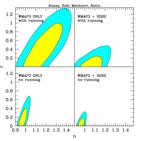
If we allow running the main effect is to open the contours toward higher value of $n$ and $r$. With running, marginalizing over all the remaining nuisance parameters, we constrain $n$ and $r$ to $1.02<n<1.38$ and $r<1.09$ at $95$% C.L. for WMAP3 alone and $0.97<n<1.21$ and $r<0.38$ in the case of WMAP3 plus SDSS.

Table 1: One-dimensional confidence limits on inflationary parameters, marginalized over all other parameters, for WMAP3 alone and WMAP3 + SDSS.

no running/	limits on $n$, $r$	data
running	95% C.L.	set
	$0.94<n<1.04$	WMAP3 ONLY
	$r<0.60$	WMAP3 ONLY
no running
	$0.93<n<1.01$	WMAP3 + SDSS
	$r<0.31$	WMAP3 + SDSS
	$1.02<n<1.38$	WMAP3 ONLY
	$r<1.09$	WMAP3 ONLY
	$-0.17<dn/d\ln k<-0.02$	WMAP3 ONLY
running
	$0.97<n<1.21$	WMAP3 + SDSS
	$r<0.38$	WMAP3 + SDSS
	$-0.13<dn/d\ln k<0.007$	WMAP3 + SDSS

Models with $n=1$ are therefore in very good agreement with CMB data in the presence of a tensor component or running different from zero. Of particular interest is the Harrison–Zel’dovich (HZ) model: $n=1$, $r=0$, $dn/d\ln k=0$. As we see from the bottom panel of Fig. 1, pure HZ spectra are not ruled out at more than 95% C.L. from CMB data alone. In particular, we found that, considering the whole sets of models in our $8$-D chain, the HZ best-fit model is at $\Delta\chi^{2}/2=2.04$, $2.77$, and $3.96$ with respect to the the best fit in the case of no running and no tensors, including tensors but no running and including tensors and running. When we include the SDSS data we found that the HZ best fit model is at $\Delta\chi^{2}/2=3.07$ with respect to the best fit in the case of no running and no tensor, $\Delta\chi^{2}/2=3.4$ with respect to the best fit with no running and $\Delta\chi^{2}/2=5.1$ with respect to the overall best fit. Since $\Delta\chi^{2}/2=6.4$ at $95.4$% confidence level for $6$ degrees of freedom, those numbers clearly indicate that even when the SDSS data is included, the HZ spectrum is in reasonable agreement with the data.

The fact that the scale-invariant value $n=1$ is consistent with the data at the 95% C.L. when no running is imposed, considerably weakens the bounds on inflationary models found in Ref. alabidi where the original WMAP3 error bars were adopted concluding that $n=1$ was ruled out at more than 99% C.L.

Figure 2: Constraints on the $n$—$dn/d\ln k$ plane for different choices of experimental datasets. The shaded regions indicate 68% and 95% C.L.

Figure 3: Constraints on the $dn/d\ln k$—$r$ plane for different choices of experimental datasets. The shaded regions indicate 68% and 95% C.L.

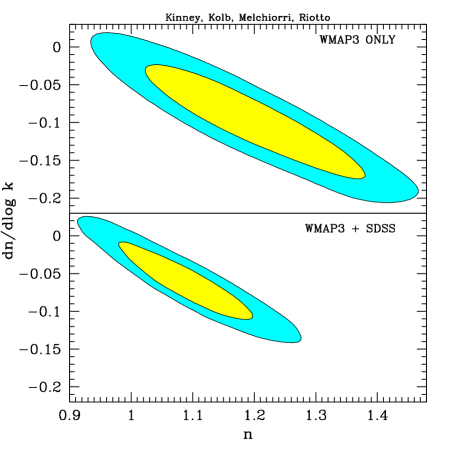
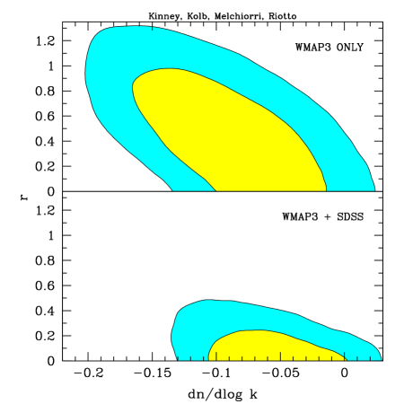
In Fig. 3 and Fig. 3 a degeneracy is evident: an increase in the spectral index $n$ is equivalent to a negative scale dependence ($dn/d\ln{k}<0$). We emphasize, however, that this behavior depends strictly on the position of the pivot scale $k_{0}$: choosing $k_{0}=0.05h$ Mpc^-1 would change the direction of the degeneracy. Models with $n\sim 1.1$ need a negative running at more than about the 95% C.L. (about $4\sigma$ in the case of WMAP3+SDSS). It is interesting also to note that models with a red spectral index, $n<1.0$, are in better agreement with the data with a zero or positive running (see Fig. 13), while models with a sizable gravity wave background need a negative running (see Fig. 3). For the WMAP3 alone case the running is bounded by $-0.02\gtrsim dn/d\ln{k}\gtrsim-0.17$ at 95% C.L. ($0.007\gtrsim dn/d\ln{k}\gtrsim-0.13$ for WMAP3+SDSS). We found that the best fit from WMAP3 alone with $dn/d\ln k=0$ is at $\Delta\chi^{2}/2=1.2$ ($\Delta\chi^{2}/2=0.2$ when including SDSS) with respect to the overall best fit. The current data, therefore, do not suggest the presence of running at more than 95% C.L.

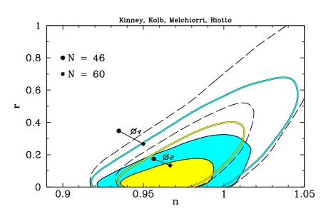
Finally, we compare our results with those presented in Spergel, et al. wmap3cosm . While there is qualitatively good agreement, a tension appears when we compare our contour plots in Fig. 4 (the no running case) with those presented in Fig. $14$ of Ref. wmap3cosm . Models with a pure HZ spectrum appear to be ruled out by WMAP3 alone at about the 99% C.L. in Ref. wmap3cosm , while our analysis indicates broader contours, with the Harrison-Zel’dovich spectrum inside the 95% C.L. region. Similarly, the contours in Ref. wmap3cosm appear to rule out $V(\phi)=\lambda\phi^{4}$, while our analysis indicates that this potential is still marginally consistent with the WMAP3 data alone at 95% confidence. In order to better understand this discrepancy, we compared our results directly with the chains made public by the WMAP team and available at the Lambda web site. We found that the error contours derived from the publicly available chains are considerably larger than those shown in Fig. 14 of Ref. wmap3cosm : error contours from our analysis of the WMAP chains are plotted as dashed lines in Fig. 4. None of the contours are as tight as those shown in Spergel et al., and the discrepancy is significant enough to influence important conclusions about the model space, in particular, the consistency of a Harrison-Zel’dovich spectrum with the data. There appears to be a clear inconsistency between our results and contours shown in Spergel et al., Figs. $12$ and $14$.

Figure 4: The $n$,$r$ parameter space WMAP3 alone (open contours) and WMAP3 + SDSS (filled contours), with a prior of $dn/d\ln{k}=0$. The line segments show the predictions for $V(\phi)=m^{2}\phi^{2}$ and $V(\phi)=\lambda\phi^{4}$ for $N=[46,60]$. The dashed lines show the 68% C.L. and 95% C.L. contours from the chains made public by the WMAP team, which do not include an HST prior on $H_{0}$ or an age prior. The scale of the plot is chosen to allow direct comparison with Fig. $14$ of Spergel et al. wmap3cosm . The shaded regions indicate 68% and 95% C.L.

V Monte Carlo reconstruction

In this section we describe Monte Carlo reconstruction, a stochastic method for “inverting” observational constraints to determine an ensemble of inflationary potentials compatible with observation. The method is described in more detail in Refs. kinney02 ; easther02 . In addition to encompassing a broader set of models than we considered in the previous section, Monte Carlo reconstruction allows us easily to incorporate constraints on the running of the spectral index $dn/d\ln{k}$ as well as to include effects to higher order in slow roll.

We have defined the slow-roll parameters $\epsilon$ and $\eta$ in terms of the Hubble parameter $H\left(\phi\right)$ in a previous section. Taking higher derivatives of $H$ with respect to the field, we can define an infinite hierarchy of slow roll parameters liddle94 :

$$\sigma \equiv {m_{\rm Pl}\over\pi}\left[{1\over 2}\left({H^{\prime\prime}\over H}\right)-\left({H^{\prime}\over H}\right)^{2}\right],$$ (27)

$${}^{\ell}\lambda_{\rm H} \equiv \left({m_{\rm Pl}^{2}\over 4\pi}\right)^{\ell}{\left(H^{\prime}\right)^{\ell-1}\over H^{\ell}}{d^{(\ell+1)}H\over d\phi^{(\ell+1)}}.$$ (28)

Here we have chosen the parameter $\sigma\equiv 2\eta-4\epsilon\simeq n-1$ to make comparison with observation convenient.

It is convenient to use $N$ as the measure of time during inflation. As above, we take $t_{e}$ and $\phi_{e}$ to be the time and field value at end of inflation. Therefore, $N$ is defined as the number of e-folds before the end of inflation, and increases as one goes backward in time ($dt>0\Rightarrow dN<0$):

$${d\over dN}={d\over d\ln a}={m_{\rm Pl}\over 2\sqrt{\pi}}\sqrt{\epsilon}{d\over d\phi},$$ (29)

where we have chosen the sign convention that $\sqrt{\epsilon}$ has the same sign as $H^{\prime}\left(\phi\right)$:

$$\sqrt{\epsilon}\equiv+{m_{\rm PL}\over 2\sqrt{\pi}}{H^{\prime}\over H}.$$ (30)

Then $\epsilon$ itself can be expressed in terms of $H$ and $N$ simply as

$${1\over H}{dH\over dN}=\epsilon.$$ (31)

Similarly, the evolution of the higher-order parameters during inflation is determined by a set of “flow” equations hoffman00 ; schwarz01 ; kinney02 ,

$${d\epsilon\over dN} = \epsilon\left(\sigma+2\epsilon\right),$$ (32)

$${d\sigma\over dN} = -5\epsilon\sigma-12\epsilon^{2}+2\left({}^{2}\lambda_{\rm H}\right),$$ (33)

$${d\left({}^{\ell}\lambda_{\rm H}\right)\over dN} = \left[\frac{\ell-1}{2}\sigma+\left(\ell-2\right)\epsilon\right]\left({}^{\ell}\lambda_{\rm H}\right)+{}^{\ell+1}\lambda_{\rm H}.$$ (34)

The derivative of a slow roll parameter at a given order is higher order in slow roll.

A boundary condition can be specified at any point in the inflationary evolution by selecting a set of parameters $\epsilon,\sigma,{}^{2}\lambda_{\rm H},\ldots$ for a given value of $N$. This is sufficient to specify a “path” in the inflationary parameter space that specifies the background evolution of the spacetime. Taken to infinite order, this set of equations completely specifies the cosmological evolution, up to the normalization of the Hubble parameter $H$. Furthermore, such a specification is exact, with no assumption of slow roll necessary. In practice, we must truncate the expansion at finite order by assuming that the ${}^{\ell}\lambda_{\rm H}$ are all zero above some fixed value of $\ell$. We choose initial values for the parameters at random from the following ranges:

$$N = [46,60]$$ (35)

$$\epsilon = \left[0,0.8\right]$$ (36)

$$\sigma = \left[-0.5,0.5\right]$$ (37)

$${}^{2}\lambda_{\rm H} = \left[-0.05,0.05\right]$$ (38)

$${}^{3}\lambda_{\rm H} = \left[-0.025,0.025\right],$$ (39)

$$\cdots$$ (40)

$${}^{M+1}\lambda_{\rm H} = 0.$$ (41)

Here the expansion is truncated to order $M$ by setting ${}^{M+1}\lambda_{\rm H}=0$. In this case, we still generate an exact solution of the background equations, albeit one chosen from a subset of the complete space of models. This is equivalent to placing constraints on the form of the potential $V\left(\phi\right)$, but the constraints can be made arbitrarily weak by evaluating the expansion to higher order. For the purposes of this analysis, we choose $M=5$. The results are not sensitive to either the choice of order $M$ (as long as it is large enough) or to the specific ranges from which the initial parameters are chosen.

Solutions to the truncated flow equations are solutions for which all of the derivatives of the Hubble constant above order $M+1$ vanish:

$${d^{\ell}H\over d\phi^{\ell}}=0,\ \ell\geq M+2,$$ (42)

with a simple polynomial solution Liddle:2003py ,

$$H\left(\phi\right)=H_{0}\left(1+A_{1}\phi+\cdots+A_{M+1}\phi^{M+1}\right).$$ (43)

The Hamilton-Jacobi Equation (5) can be applied to this solution to derive an analytic form for the potential in terms of the parameters $A_{1},\ldots,A_{M+1}$. The set of boundary conditions in Eq. (41) then consist of a weak slow-roll prior on the polynomial fit for $H(\phi)$: the inflaton must be slowly rolling at least at one point in its evolution. Thus, while the flow equations in and of themselves simply define an expansion in $H(\phi)$, the choice of boundary condition and the requirement that inflation last at least 46 e-folds comprise a well-defined physical prior on the inflationary model space.

Some interesting recent papers have explored alternative methods for constraining the “model space” of inflation. In particular, Ref. Peiris:2006ug incorporates the lowest-order flow parameters directly into the Monte Carlo Markov Chain fit, although they do not include effects to higher order in slow roll. Refs. Parkinson:2006ku ; Pahud:2006kv apply a Bayesian model selection approach to the problem, but also do not consider higher-order effects which in principle contribute to a running spectral index. Our analysis extends these results by including running of the spectral index as well as effects to higher order in slow roll.

Once we obtain a solution to the flow equations $[\epsilon(N),\sigma(N),{}^{\ell}\lambda_{\rm H}(N)]$, we can calculate the predicted values of the tensor/scalar ratio $r$, the spectral index $n$, and the “running” of the spectral index $dn/d\ln k$. To lowest order, the relationship between the slow roll parameters and the observables is especially simple: $r=16\epsilon$, $n-1=\sigma$, and $dn/d\ln k=0$. To second order in slow roll, the observables are given by liddle94 ; stewart93 ,

$$r=16\epsilon\left[1-C\left(\sigma+2\epsilon\right)\right]$$ (44)

for the tensor/scalar ratio, and

$$n-1=\sigma-\left(5-3C\right)\epsilon^{2}-{1\over 4}\left(3-5C\right)\sigma\epsilon+{1\over 2}\left(3-C\right)\left({}^{2}\lambda_{\rm H}\right)$$ (45)

for the spectral index. The constant $C\equiv 4(\ln{2}+\gamma)-5=0.0814514$, where $\gamma\simeq 0.577$ is Euler’s constant. Derivatives with respect to wavenumber $k$ can be expressed in terms of derivatives with respect to $N$ as liddle95

$${d\over dN}=-\left(1-\epsilon\right){d\over d\ln k}.$$ (46)

The scale dependence of $n$ is then given by the simple expression

$${dn\over d\ln k}=-\left({1\over 1-\epsilon}\right){dn\over dN},$$ (47)

which can be evaluated by using Eq. (45) and the flow equations. For example, for the case of $V\propto\phi^{4}$, the observables to lowest order are

$$r \simeq {16\over N+1},$$ (48)

$$n-1 \simeq -{3\over N+1},$$ (49)

$${dn\over d\ln k} \simeq -{3\over N\left(N+1\right)}.$$ (50)

The final result following the evaluation of a particular path in the $M$-dimensional “slow-roll space” is a point in “observable parameter space,” i.e., $(r,n,dn/d\ln k)$, corresponding to the observational prediction for that particular model.

The reconstruction method works as follows:

1. Specify a “window” of parameter space: e.g., central values for $n-1$, $r$, or $dn/d\ln{k}$ and their associated error bars.

2. Select a random point in slow roll space, $[\epsilon,\eta,{}^{\ell}\lambda_{\rm H}]$, truncated at order $M$ in the slow roll expansion.

3. Evolve forward in time ($dN<0$) until either (a) inflation ends ($\epsilon>1$), or (b) the evolution reaches a late-time fixed point ($\epsilon={}^{\ell}\lambda_{\rm H}=0,\ \sigma={\rm const.}$).

4. If the evolution reaches a late-time fixed point, calculate the observables $r$, $n-1$, and $dn/d\ln k$ at this point.

5. If inflation ends, evaluate the flow equations backward $N$ e-folds from the end of inflation. Calculate the observable parameters at that point.

6. If the observable parameters lie within the specified window of parameter space, compute the potential and add this model to the ensemble of “reconstructed” potentials.

7. Repeat steps 2 through 6 until the desired number of models have been found.

We performed the Monte Carlo reconstruction using the more restrictive of the data sets considered, combining the WMAP3 data with the Sloan Digital Sky Survey. We ran the reconstruction code long enough (10,703,502 iterations) to collect 10,000 models consistent with the WMAP3 + SDSS error bars: 4115 are within the 68% C.L. contours, and 5885 are within the 95% C.L. contours.

To illustrate the degree of overlap between the various classes of model, the predictions for different models are shown in the top panel of Fig. 5, including the effect of the uncertainty in the number of e-folds $N$. The different classes of potential do not have significant overlap, and it is therefore possible to distinguish one from another observationally.

Figure 5 also shows the points generated by Monte Carlo Reconstruction in the $n,r$ parameter space. Since there is no measure on the space of initial conditions, the distribution of points generated by the flow equations cannot be interpreted in a rigorously statistical fashion: the error bars are those generated from the data using COSMOMC, and the points plotted are points generated by the flow equations consistent with those errors, including running of the spectral index as a parameter. The clustering of the models in the parameter space, however, is significant: selecting models based on even an extremely weak assumption of slow-roll results in a strong clustering of the models in the region favoring a red spectrum and $dn/d\ln{k}=0$.

In this sense, the preference for running and a blue spectrum present in the data itself contains very little information relevant to constraining slow-roll inflation models: it can be interpreted simply an artifact of an “accidental” parameter degeneracy in the data. Allowing running as a parameter but assuming slow roll inflation gives constraints on the inflationary model space largely consistent with an analysis which assumes negligible running as a prior on the parameter space from the beginning. In other words: there is no evidence for inflation with a measurable running of the spectral index.

Figure 5: Inflationary models plotted against the 68% and 95% WMAP3 + SDSS error contours. Top panel: the predictions of various specific inflationary potentials (solid bands) plotted against the error bars from WMAP3 + SDSS with a prior of $dn/d\ln{k}=0$. Bottom panel: 10,000 models generated by flow Monte Carlo consistent with the WMAP3 + SDSS data sets including running as a parameter, indicated by the larger error contours. The contours with a $dn/d\ln{k}=0$ prior are plotted as a reference, and were not used in the Monte Carlo reconstruction. (Some data points fall outside the error contours plotted because likelihoods for the models were calculated using the full three-dimensional likelihood function ${\cal L}(n,r,dn/d\ln{k})$, and the contours were obtained by marginalizing over $dn/d\ln{k}$).

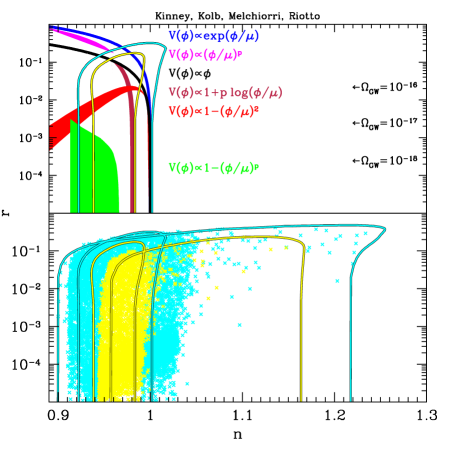
From the flow equations (34) it is evident that the line along the $r=0$ axis, with $\epsilon={}^{\ell}\lambda_{\rm H}=0$ is a fixed point of the flow evolution, including taking the flow equations to infinite order. For parameters on the “red” side of scale invariance, i.e. $\sigma<0$, this fixed point is unstable: flow moves away from the fixed point as $N\rightarrow 0$, and toward the fixed point as $N\rightarrow\infty$. Conversely, the fixed point for $\sigma>0$ is stable: models evolve toward this fixed point at late times, $N\rightarrow 0$. Integrating the flow equations forward in time yields one of two possible outcomes. One possibility is that the condition $\epsilon=1$ may be satisfied for some finite value of $N$, which defines the end of inflation. We identify this point as $N=0$ so that the primordial fluctuations are actually generated when $N=[46,60]$. Alternatively, the solution can evolve toward an inflationary fixed point with $r=0$ and $n>1$, in which case inflation never stops. In reality, inflation must stop at some point, presumably via some sort of instability, such as the “hybrid” inflation mechanism linde91 ; linde94 ; copeland94 ; lr97 . Examples of potentials which fall into this class of models are the simplest hybrid potentials,

$$V\left(\phi\right)=\Lambda^{4}\left[1+\left({\phi\over\mu}\right)^{p}\right].$$ (51)

Here we take the observables for such models to be the values at the late-time attractor. Since models on the attractor are by definition those for which the variation in the slow roll parameters with $N$ vanishes, such models also predict zero running of the scalar spectral index. We find that the WMAP3 data strongly disfavor models which evolve to a late-time asymptote with $r=0$, $n>1$, and $dn/d\ln{k}=0$. The $95$% confidence limit for a blue spectrum with no tensors and no running (i.e., not marginalized over $r$) from WMAP3 alone is $n<1.0007$, and from WMAP3 + SDSS is $n<1.001$. Of more than ten million models tested, only one model consistent with the data relaxed to the late-time asymptote, with a spectral index $n=1.0004$ and $r=0.0000002$; for all intents and purposes a Harrison-Zel’dovich spectrum. Every other model in the Monte Carlo reconstruction set was of the “nontrivial” type, with inflation ending naturally by evolving through $\epsilon=1$ at late times. We note that the level of running required to accommodate a blue spectrum is severe: even dynamical supersymmetric inflation, which predicts a blue spectrum and negative running [Eq. (24)], does not produce a strong enough running to match the data, and is also ruled out to more than 95% C.L. by WMAP3 + SDSS for $n>1.001$.

Figure 6: Potentials generated by Monte Carlo Reconstruction consistent with WMAP3 + SDSS to 68% C.L. in the light shaded (yellow) region and 95% C.L. in the darker shaded (cyan) region. The WMAP3 data place an upper limit of about $2\times 10^{16}\ {\rm GeV}$ on the energy scale of inflation. No lower limit is possible without a detection of a tensor mode signal. The concave-up line at the bottom of the figure is the single model in $10^{7}$ models generated which converged to an inflationary fixed point at late time.

We can also place constraints on the energy scales relevant to inflation, in particular the “height” of the potential $V\sim\Lambda^{4}$, and the “width” of the potential, typically quantified as the field variation $\Delta\phi$ during inflation. Given a path in the slow roll parameter space, the form of the potential is fixed, up to normalization hodges90 ; copeland93 ; beato00 ; easther02 . The starting point is the Hamilton-Jacobi equation,

$$V(\phi)=\left({3m_{\rm Pl}^{2}}\over 8\pi\right)H^{2}(\phi)\left[1-{1\over 3}\epsilon(\phi)\right].$$ (52)

We have $\epsilon(N)$ trivially from the flow equations. In order to calculate the potential, we need to determine $H(N)$ and $\phi(N)$. With $\epsilon$ known, $H(N)$ can be determined by inverting the definition of $\epsilon$, Eq. (31). Similarly, $\phi(N)$ follows from the first Hamilton-Jacobi equation, Eq. (4):

$${d\phi\over dN}={m_{\rm PL}\over 2\sqrt{\pi}}\sqrt{\epsilon}.$$ (53)

Using these equations and Eq. (52), the form of the potential can then be fully reconstructed from the numerical solution for $\epsilon(N)$. The only necessary observational input is the normalization of the Hubble parameter $H$, which enters the above equations as an integration constant. Here we use the simple condition that the density fluctuation amplitude (as determined by a first-order slow roll expression) be of order $10^{-5}$,

$${\delta\rho\over\rho}\simeq{H\over m_{\rm Pl}}\frac{1}{\sqrt{\pi\epsilon}}=10^{-5}.$$ (54)

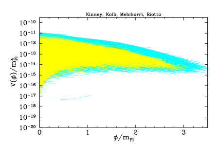
A more sophisticated treatment would perform a full normalization to the CMB data bunn94 ; stompor95 . The value of the field, $\phi$, also contains an arbitrary, additive constant. Fig. 6 shows the reconstructed potentials consistent with the WMAP3 + SDSS data set.

We see that the energy scale for inflation favored by the flow Monte Carlo gives $V_{0}$ between $5\times 10^{14}\ {\rm GeV}$ and $2\times 10^{16}\ {\rm GeV}$, although without a detection of a nonzero tensor/scalar ratio, it is not possible to put a purely observational lower limit on the height of the inflationary potential. Inflationary potentials with very low energy scales (in particular those with $\Delta\phi\ll m_{\rm Pl}$ during inflation) require the imposition of a symmetry to suppress the mass term for the inflaton Knox:1992iy ; Kinney:1995cc ; Easther:2006qu . Such potentials (corresponding to the region labeled $V(\phi)\propto 1-(\phi/\mu)^{p}$ in Fig. 5) are consistent with the WMAP3 data and predict an unobservably small value for the tensor/scalar ratio $r$. Even if one wished to consider such models fine-tuned (see, e.g. Ref. Efstathiou:2006ak ) and therefore disfavored, the range of energy scales favored by the flow Monte Carlo (Fig. 6) is consistent with tensor/scalar ratios as low as $r\sim 10^{-5}$, a level unlikely to be detectable by any currently foreseen experiments. Refs. Boyle:2005ug ; Bock:2006yf suggest that fine-tuning considerations force the tensor/scalar ratio for a red spectrum to detectable levels of $r\sim 0.01$. We see no evidence of such an effect in the flow analysis, for which no explicit tuning of the potential is performed.

VI Conclusions

In this paper, we presented an analysis of the recent WMAP three-year data set with an emphasis on parameters relevant for distinguishing among the various possible models for inflation. Our results are in good agreement with other analyses of the data Lewis:2006ma ; Seljak:2006bg , but show significant inconsistencies with the results reported by the WMAP team in Figs. $12$ and $14$ of Ref. wmap3cosm .

We found that the WMAP3 data alone are consistent within 95% C.L. with a scale-invariant power spectrum, $n=1$, with no running of the spectral index, $dn/d\ln{k}=0$ and no tensor component. The Harrison-Zel’dovich spectrum is therefore still not ruled out at high significance, a conclusion in accord with Refs. Parkinson:2006ku ; Magueijo:2006we . While a detection of a running spectral index would be of great significance for inflationary model building Easther:2006tv ; Cline:2006db , no clear evidence for running is present in the WMAP3 data. The data are, however, consistent with strongly negative running combined with a large tensor/scalar ratio and a “blue” power spectrum.

The inclusion of the Sloan Digital Sky Survey datasets in the analysis has the effect of reducing the error bars and gives a better determination of the inflationary parameters. For instance, the inclusion of SDSS rules out quartic chaotic models of inflation of the form $V(\phi)\sim\lambda\phi^{4}$. Chaotic inflation with a quadratic potential $V(\phi)\sim m^{2}\phi^{2}$ is consistent with all datasets considered.

In addition, we applied the Monte Carlo reconstruction technique to generate an ensemble of inflationary potentials consistent with observation. Our results may be summarized as follows: Models which evolve to a late-time fixed point in the space of flow parameters are strongly disfavored by the data. Of more than 10 million models analyzed in the flow Monte Carlo, one evolved to a late-time inflationary asymptote indistinguishable from a Harrison-Zel’dovich spectrum. The rest were characterized by a dynamical end to inflation, with the first slow-roll parameter $\epsilon$ evolving to unity in finite time. The late-time attractor in flow space corresponds to models with a “blue” power spectrum ($n>1$) and negligible $r$ and $dn/d\ln{k}$, and we conclude that such models are inconsistent with the data for $n>1.001$. This is a significant constraint on the inflationary model space. In particular, the data rule out the simplest models of hybrid inflation of the form $V(\phi)=V_{0}+m^{2}\phi^{2}$ as well as models such as $V(\phi)\propto 1+(\mu/\phi)^{p}$, which predict some negative running. This of course does not rule out all models for which inflation ends via a hybrid mechanism. Some hybrid models are characterized by a red spectrum, for example “inverted” hybrid models and models with logarithmic potentials inspired by (global) supersymmetry. Finally, we find that there is no evidence to support any lower bound on the amplitude of gravitational waves. Tensor/scalar ratios as low as $r\sim 10^{-5}$ were produced by the flow Monte Carlo without explicit tuning of the inflationary potential.