Markov chain Monte Carlo analysis of Bianchi ${\rm VII_{h}}$ models

Abstract

We have extended the analysis of Jaffe et al. (2005a, 2006) to a complete Markov chain Monte Carlo (MCMC) parameter space study of the Bianchi type ${\rm VII_{h}}$ models including a dark energy density, using Wilkinson Microwave Anisotropy Probe (WMAP) cosmic microwave background (CMB) data from the 1-year and 3-year releases. Since we perform the analysis in a Bayesian framework our entire inference is contained in the multidimensional posterior distribution from which we can extract marginalised parameter constraints and the comparative Bayesian evidence. Treating the left-handed Bianchi CMB anisotropy as a template centred upon the ‘cold-spot’ in the southern hemisphere, the parameter estimates derived for the total energy density, ‘tightness’ and vorticity from 3-year data are found to be: $\Omega_{tot}=0.43\pm 0.04$, $h=0.32^{+0.02}_{-0.13}$, $\omega=9.7^{+1.6}_{-1.5}\times 10^{-10}$ with orientation $\gamma={337^{\circ}}^{+17}_{-23}$). This template is preferred by a factor of roughly unity in log-evidence over a concordance cosmology alone. A Bianchi type template is supported by the data only if its position on the sky is heavily restricted. All other Bianchi ${\rm VII_{h}}$ templates including all right handed models, are disfavoured. The low total energy density of the preferred template, implies a geometry that is incompatible with cosmologies inferred from recent CMB observations. Jaffe et al. (2005b) found that extending the Bianchi model to include a term in $\Omega_{\Lambda}$ creates a degeneracy in the $\Omega_{m}-\Omega_{\Lambda}$ plane. We explore this region fully by MCMC and find that the degenerate likelihood contours do not intersect areas of parameter space that 1 or 3 year WMAP data would prefer at any significance above $2\sigma$. Thus we can confirm the conclusion that a physical Bianchi ${\rm VII_{h}}$ model is not responsible for this signature, which we have treated in our analysis as merely a template.

1 Introduction

It has recently been proposed that some of the current anomalous results seen in observations of the CMB sky by WMAP, namely non-Gaussian structure centered on the so called ‘cold spot’ in the southern hemisphere (Vielva et al. 2005; Cruz et al. 2005), low quadrupole (Efstathiou, 2004) and multipole alignments (de Oliveira-Costa et al., 2003), could be removed by allowing for large scale vorticity and shear. Components such as these arise in Bianchi type ${\rm VII_{h}}$ models (Barrow et al., 1985) due to large scale rotation of the universe distorting the CMB since the time of last scattering. This assumption has the unfortunate side-effect of violating universal isotropy and hence the cosmological principle, so any such result should be examined very carefully.

Such a finding was indeed made by Jaffe et al. (2005a) [hereafter referred to as Jaffe] where a significant correlation was found between a class of Bianchi ${\rm VII_{h}}$ models and WMAP observations. However the resultant best-fit Bianchi component was derived directly from Barrow et al. (1985) for a universe with a large negative curvature with total energy density $\Omega_{tot}=0.5$ and including no dark energy component. Such a cosmology cannot be reconciled with cosmologies inferred from either current CMB or other astronomical observations. In Jaffe et al. (2005b) the authors extended their study to include a cosmological constant and searched for a morphologically identical template to their first analysis in the increased parameter space. We perform a new study to explore fully the parameter space of both Bianchi and cosmological parameters in order to select the best fitting template. We carry out this investigation using Markov chain Monte Carlo (MCMC) sampling in a fully Bayesian manner. Hence we also find the comparative Bayesian evidence allowing an assessment of whether the inclusion of such a template is supported by the data.

2 MCMC Analysis and Model Selection Framework

Several recent studies have been performed using a Bayesian approach to cosmological parameter estimation and model selection (Jaffe 1996, Drell et al. 2000, John & Narlikar 2002, Slosar et al. 2003, Saini et al. 2004, Marshall et al. 2003, Niarchou et al. 2004, Basset et al. 2004, Mukherjee et al. 2005, Trotta 2005, Beltran et al. (2005), Bridges et al. 2005, Parkinson et al. 2006). Here we are interested in determining the best fitting Bianchi ${\rm VII_{h}}$ sky from WMAP data using a selection of all sky maps available; the 1-year WMAP Internal Linear Combination (WILC) map (Bennett et al., 2003), the Lagrange Internal Linear Combination (LILC) map (Eriksen et al., 2004), the Tegmark, de Oliveira-Costa & Hamilton (TOH) map (Tegmark et al., 2003), the Maximum Entropy Method (MEM) map (Stolyarov et al., 2005) and the new 3-year WILC map (Hinshaw et al., 2006). We have incorporated Bianchi sky simulations into an adapted version of the cosmoMC package (Lewis & Bridle, 2002) which we show via simulated sky maps is capable of extracting both the underlying cosmology and the Bianchi signal, while also determining when the addition of such a component is favoured by the data.

The Bayesian framework allows the examination of a set of data $\bf{D}$ under the assumption of a model $M$ defined by a set of parameters $\bf{\Theta}$ with Bayes’ Theorem:

$$P(\bf{\Theta|\bf{D},M})=\frac{P(\bf{D}|\bf{\Theta},M)P(\bf{\Theta}|M)}{P(\bf{D}|M)},$$ (1)

where $P(\bf{\Theta}|\bf{D},M)$ is the posterior distribution, $P(\bf{D}|\bf{\Theta},M)$ the likelihood, $P(\bf{\Theta}|M)$ the prior and $P(\bf{D}|M)$ the Bayesian evidence. We explore the parameter space by MCMC sampling to maximise the likelihood utilising a reasonable convergence criteria from the Gelman & Rubin $R$ statistic (Gelman & Rubin, 1992) so that once the Markov chain has reached its stationary distribution, samples from it reliably reflect the actual posterior distribution of the model. The final result will be parameter estimates marginalised from the multi-dimensional posterior and a value of the evidence for the model being studied.

2.1 Likelihood

A CMB experiment records the temperature anisotropy on the sky $\bf{T}(\bf{\hat{p}})$. We wish to find a cosmological model that can optimally describe these fluctuations by maximising the probability of observing the data $\bf{T}(\bf{\hat{p}})$ given a model described by a set of parameters $\bf{\Theta}_{\rm{C}}$. Then for a Gaussian model, from Bayes’ Theorem we can express this probabilty, the likelihood, as:

$$P(\bf{T}(\bf{\hat{p}})|\bf{\Theta}_{\rm{C}})\propto\frac{1}{\sqrt{|\mathcal{C}|}}e^{-\frac{1}{2}(\bf{T}^{\rm T}\mathcal{C}^{-1}\bf{T})}$$ (2)

where $\mathcal{C}$ is the covariance matrix containing the predictions of the model $\bf{\Theta}_{\rm{C}}$ and $|\mathcal{C}|$ its determinant. Expanding the temperature sky in spherical harmonmics $\bf{T}(\bf{\hat{p}})=\sum_{lm}a_{lm}Y_{lm}$, in a universe that is globally isotropic means $\mathcal{C}_{lm,l^{\prime}m^{\prime}}=\langle a_{lm}a^{*}_{l^{\prime}m^{\prime}}\rangle=C_{l}\delta_{ll^{\prime}}\delta_{mm^{\prime}}$ where the variance of the harmonic coefficients $a_{lm}$ is $C_{l}=\frac{1}{2l+1}\sum_{m}|a_{lm}|^{2}$. Thus Eqn. 2 becomes :

$$P(\{\hat{a}_{lm}\}|{\bf{\Theta}_{\rm{C}}})\propto\prod_{lm}\frac{e^{\left(-|\hat{a}_{lm}|^{2}/2C_{l}\right)}}{\sqrt{C_{l}}}.$$ (3)

If one assumes universal isotropy the likelihood is then independent of $m$ which can be summed over to give (for a full sky survey) the form used in most conventional CMB analyses:

$$\ln P(\hat{C_{l}}|{\bf{\Theta}_{\rm{C}}})=(2l+1)\left(\frac{\hat{C_{l}}}{C_{l}}+\ln|C_{l}|\right),$$ (4)

where $\hat{C}_{l}$ is the observed quantity. However Bianchi $\rm{VII_{h}}$ models are anisotropic so one cannot simply compare observed $\hat{C}_{l}$’s with theoretical $C_{l}$’s, instead the full set of $a_{lm}$’s must be used.

In this analysis we make the assumption that there is both a background cosmological contribution and Bianchi $\rm{VII_{h}}$ contribution to the CMB. We take the cosmological component to be that of a standard $\Lambda$CDM universe, producing a set of $a_{lm}$’s, while the Bianchi model component (defined by parameters $\bf{\Theta}_{\rm{B}}$) is given by $a_{lm}^{\rm{B}}$. The Bianchi component can then be subtracted from the observed $\hat{a}_{lm}$’s so that Eqn 3 becomes:

$$P(\{\hat{a}_{lm}\}|\Theta_{\rm{B}},\Theta_{\rm{C}})\propto\prod_{l}\frac{1}{\sqrt{C_{l}}}e^{-\left(\frac{(\hat{a}_{l0}-a_{l0}^{B})^{2}}{C_{l}}\right)}\cdot\\ \prod_{m=1}^{l}\frac{2}{C_{l}}e^{-\left(\frac{|\hat{a}_{lm}-a_{lm}^{B}|^{2}}{2C_{l}}\right)}.$$ (5)

For numerical convenience we take the natural logarithm to yield the final likelihood function used in this analysis, hereafter referred to as $\mathcal{L}$:

$$\ln\mathcal{L}\propto\sum_{l}-(l+1/2)\ln(C_{l})\\ -\frac{(a_{l0}-a_{l0}^{\rm{B}})^{2}}{2C_{l}}-\frac{1}{C_{l}}\sum_{m=1}^{l}\left(|a_{lm}-a_{lm}^{\rm{B}}|^{2}\right),$$ (6)

which would reduce to Eqn. 4 if the Bianchi signal were zero.

2.2 Evidence

The Bayesian evidence is the average likelihood over the entire prior parameter space of the model:

$$\int\int{\mathcal{L}(\Theta_{\rm{C}},\Theta_{\rm{B}})P(\Theta_{\rm{C}})P(\Theta_{\rm{B}})}d^{N}\Theta_{\rm{C}}d^{M}\Theta_{\rm{B}},$$ (7)

where $N$ and $M$ are the number of cosmological and Bianchi parameters respectively. Those models having large areas of prior parameter space with high likelihoods will produce high evidence values and vice versa. This effectively penalises models with excessively large parameter spaces, thus naturally incorporating Ockam’s razor.

The results generated in this paper have employed the new method of nested sampling (Skilling, 2004) as implemented in a forthcoming publication (Shaw et al. in preperation). This method is capable of much higher accuracy than previous methods such as thermodynamic integration (see e.g. Beltran et al. 2005, Bridges et al. 2005). due to a computationally more effecient mapping of the integral in Eqn. 7 to a single dimension by a suitable re-parameterisation in terms of the prior mass $X$. This mass can be divided into elements $dX=\pi(\mathbf{\Theta})d^{N}\mathbf{\Theta}$ which can be combined in any order to give say

$$X(\lambda)=\int_{\mathcal{L\left(\mathbf{\Theta}\right)>\lambda}}\pi(\mathbf{\Theta})d^{N}\mathbf{\Theta},$$ (8)

the prior mass covering all likelihoods above the iso-likelihood curve $\mathcal{L}=\lambda$. We also require the function $\mathcal{L}(X)$ to be a singular decreasing function (which is trivially satisfied for most posteriors) so that using sampled points we can estimate the evidence via the integral:

$$\mathcal{Z}=\int_{0}^{1}{\mathcal{L}(X)}dX.$$ (9)

Via this method we can obtain evidences with an accuracy 10 times higher than previous methods for the same number of likelihood evaluations.

3 Bianchi ${\rm VII_{h}}$ Simulations

Jaffe implemented solutions of the geodesic equations developed by Barrow et al. (1985) to compute Bianchi induced temperature maps in type ${\rm VII_{h}}$ cases. Jaffe et al. (2005b) extended these to include cosmologies with dark energy allowing an almost flat geometry, in keeping with the so called concordance cosmology. One of us (ANL, in preparation) independently performed the same extension and found results agreeing well with Jaffe et al. (2005b).

The models are parameterised by six independent quantities; the total energy density $\Omega_{tot}$ = $\Omega_{m}$ + $\Omega_{\Lambda}$, the current vorticity $\omega$, $h$ which determines the ‘tightness’ of the spiral and the Euler angles $\alpha$ and $\beta$ determining the position of the centre of the spiral on the sky with $\gamma$ allowing rotation of the pattern about this point . In addition one must specify the direction of rotation or ‘handedness’ of the spiral. The ratio of the current shear to the Hubble parameter $(\sigma/H)_{0}$ (differential expansion) is determined by the combination of these parameters:

$$\left(\frac{\sigma}{H}\right)_{0}=\frac{6h\Omega_{tot}}{\sqrt{2}(1+h)^{1/2}(1+9h)^{1}/2(1-\Omega_{tot})}\left(\frac{\omega}{H}\right)_{0}.$$

Jaffe found a best fit bianchi template $\bf{T}$ by a $\chi^{2}$ analysis of the observed CMB sky $\bf{D}$ for a selection of WMAP data variants by minimising:

$$\chi^{2}=(\bf{D}-\bf{T})^{T}\bf{M}^{-1}(\bf{D}-\bf{T})$$ (10)

under the assumption of an embedded cosmology $\bf{M}$ given by the best fit 1-year WMAP angular power spectrum (Spergel et al., 2003). There is no contribution from noise in this expression as the dominant uncertainty on large scales is from cosmic variance. Their result is shown in Fig. 1 computed in our formalism with parameters $\Omega_{tot}=0.5$, $\omega=10.38\times 10^{-10}$, $h=0.15125$ and position ($42^{\circ}$, $28^{\circ}$, $310^{\circ}$) in Euler angles. The primary feature is a central core positioned on the so called ‘cold spot’, assumed to be the source of a large area of non-gaussianity. The corrected map (see Fig. 2), produced after removal of this Bianchi ‘contamination’, provides even by cursory visual inspection a more statistically homogeneous sky.

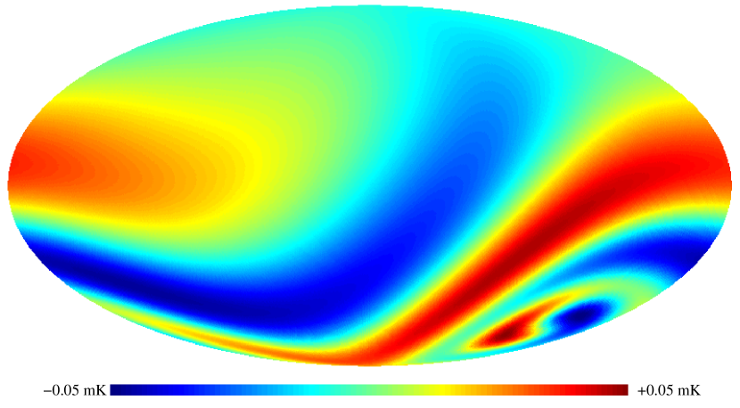
Figure 1: Best fit bianchi template as found by Jaffe et al. (2006) computed from parameters $\Omega_{tot}=0.5$, $\omega=10.38\times 10^{-10}$, $h=0.15125$ and position ($42^{\circ}$, $28^{\circ}$, $310^{\circ}$) in Euler angles.

Figure 2: Raw LILC map (left) with the Bianchi corrected map (right)

In Section 4 we will perform our analysis on simulated data in order to test our parameter recovery and model selection algorithm with a Bianchi component of varying amplitude superimposed on a background concordance cosmology. In Section 5 we perform this analysis on real data to effectively extend Jaffe’s study to fit simultaneously for a selection of right and left handed Bianchi models and a background cosmological component. This method has two main advantages over Jaffe’s original template analysis: i) confirmation of the robustness of the detection within a varying cosmology –thus accounting for possible degenerate parameters and ii) estimation of the ratio of Bayesian evidences with and without a Bianchi component –providing an effective model selection to favour or disfavour the inclusion of a such an addition to the standard model.

4 Simulated Data

A set of simulated CMB sky maps were produced with the HEALPix software routines. These contained a cosmic variance limited concordance cosmological component and a Bianchi $\rm{VII_{h}}$ component with fixed handedness, shear, matter and dark energy density and geometry but varying the vorticity $\omega$ to study the sensitivity of the method to the total amplitude of the Bianchi signal (of which $\omega$ is a good tracer). Evidence estimates were produced for two parameterisations: Bianchi + cosmology (model A); and cosmology only (model B).

In order to provide the best possible assessment of our method the Bianchi simulations were created with Jaffe’s best fit parameter set of: $h=0.15$, $\Omega_{m}=0.5$, $\Omega_{\Lambda}=0$, $\alpha=42^{\circ}$, $\beta=28^{\circ}$ and $\gamma=310^{\circ}$ (see Fig. 3 (a)) combined with a best fit WMAP cosmology (see Fig. 3 (b)) with eight equally spaced vorticities incremented between $5$ and $19\times 10^{-10}$ (see Fig. 3 (c)-(j)). Ultimately we aim to ascertain via these simulations the lowest amplitude of Bianchi signal we can succesfully extract via our method –where $\omega=10\times 10^{-10}$ represents the level of sensitivity required to detect a Jaffe type component in real data.

Marginalised parameter constraints (see Fig. 5) illustrate we are able to successfully extract the input Bianchi parameters for amplitudes at and above roughly $\omega=11\times 10^{-10}$, which suggests our method should be able to determine parameters of any Bianchi component similar to the Jaffe template, should one exist. As for the question of whether such an inclusion is actually warranted by the data, we consider the evidence. A useful guide has been given by Jeffreys (1961) to rank relative evidence differences in order of significance: $\Delta\mbox{ln}E<1$ inconclusive, $1<\Delta\mbox{ln}E<2.5$ significant, $2.5<\Delta\mbox{ln}E<5$ strong and $\Delta\mbox{ln}E>5$ decisive. While there is marginal evidence in these simulations for a component at $\omega=11\times 10^{-10}$ (see Table 1) a significant model selection can only be made at $\omega=13\times 10^{-10}$, also roughly at the point where the Bianchi template becomes visibly apparent in the sky maps in Fig. 3.

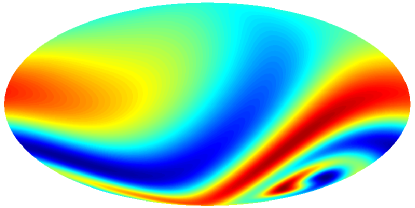
(a) Bianchi

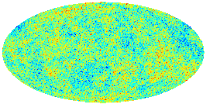
(b) Concordance cosmology

(c) $\omega=5\times 10^{-10}$

(d) $\omega=7\times 10^{-10}$

(e) $\omega=9\times 10^{-10}$

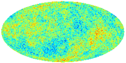
(f) $\omega=11\times 10^{-10}$

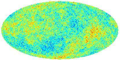
(g) $\omega=13\times 10^{-10}$

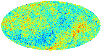
(h) $\omega=15\times 10^{-10}$

(i) $\omega=17\times 10^{-10}$

(j) $\omega=19\times 10^{-10}$

Figure 3: Simulated data created with a WMAP concordance cosmology (a) and a Bianchi component (enhanced by a factor of 10 for clarity) (b) of the type found by Jaffe with an increasing vorticity ($\omega$).

Figure 4: Comparison of the relative amplitudes of the angular power spectra ($C_{l}$) of four simulated Bianchi skies of varying vorticity and the Jaffe template.

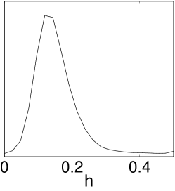
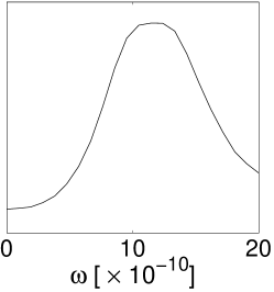
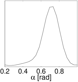
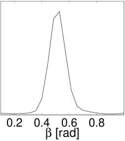
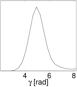
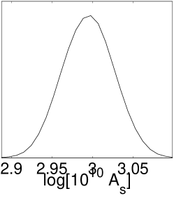
Figure 5: Extracted cosmological and Bianchi parameters from a simulated map with $\omega=11\times 10^{-10}$ (described in text).

Table 1: Differences of $\ln$ evidence with (model A) and without (model B) a Bianchi component with vorticity incremented between $5-19\times 10^{-10}$.

$\mathbf{\omega}$ $[\times 10^{-10}]$	A	B
5	0.0 $\pm 0.2$	-1.6 $\pm$ 0.3
7	0.0 $\pm 0.2$	-1.3 $\pm$ 0.3
9	0.0 $\pm 0.2$	-1.1 $\pm$ 0.3
11	0.0 $\pm 0.2$	-0.9 $\pm$ 0.3
13	0.0 $\pm 0.2$	+1.4 $\pm$ 0.3
15	0.0 $\pm 0.2$	+3.6 $\pm$ 0.3
17	0.0 $\pm 0.2$	+6.2 $\pm$ 0.3
19	0.0 $\pm 0.2$	+8.4 $\pm$ 0.3

5 Application to Real Data

The analysis was performed on both one and three year ILC maps, probing structure up to multipoles of 64, which does not limit any study of Bianchi structure, which contains few features beyond $l=20$ (see Fig. 4) but does preclude a full examination of the background cosmology. This was an unfortunate necessity of using the ILC maps owing to their complex noise properties.

As we are adopting a Bayesian approach in this analysis our results will be dependent on the prior parameter ranges chosen. Our most conservative, and thus widest uniform prior ranges are listed in Table 2. From a Bayesian point of view these are broad enough to represent the situation in which there is little prior knowledge of the Bianchi models. In particular the $h$ parameter, which decreases the spiral ‘tightness’ almost exponentially between 0.01 and 0.2 but little thereafter was given a prior range from 0.01 to 1 –encompassing the majority of possible features. The vorticity $\omega$ increases the Bianchi amplitude roughly linearly so a prior range centred on the amplitude of the Jaffe template was adopted providing a realistic upper limit of $20\times 10^{-10}$ at which point the Bianchi signal would dominate the CMB sky and a lower limit of $\omega=0$ corresponding to no Bianchi signal. Bianchi ${\rm VII_{h}}$ models are only defined in open cosmologies where $\Omega_{tot}<1$ so the prior chosen on the combination of matter and dark energy energy density was restricted to lie within $0.01$ and $0.99$ –thus introducing an implicit prior on $\Omega_{\Lambda}^{\rm B}$ of $\pm 0.8$ (as $\Omega_{\Lambda}^{\rm B}+\Omega_{m}^{\rm B}=\Omega_{tot}^{\rm B}$). The Euler angles position the centre of the spiral, via $\alpha$ and $\beta$ varied over $360^{\circ}$ and $180^{\circ}$ respectively while the orientation of the pattern is given by $\gamma$ rotating over $360^{\circ}$. In the subsequent sections we will analyse a range of Bianchi models (Table 3) defined by subsets of the above prior ranges while simultaneously fitting a scalar perturbation amplitude $A_{s}$ of an assumed background concordance cosmology. In Section 5.2 we will compare, via the evidence, models B – G with the concordance cosmology model A as to their ability to describe, adequately the observed CMB sky.

Table 2: Summary of Bianchi ${\rm VII_{h}}$ component parameters and priors.

Full Bianchi

$\Omega_{tot}^{\rm B}=[0.01,0.99]$

$\Omega_{m}^{\rm B}=[0.01,0.99]$

$h=[0.01,1]$

$\omega=[0,20]\times 10^{-10}$

$\alpha=[0,2\pi]$${\rm rads}$

$\beta=[0,\pi]$${\rm rads}$

$\gamma=[0,2\pi]$${\rm rads}$

Chirality = L/R

Table 3: Cosmological and Bianchi parameterisations for each of the parameter subsets studied.

Model	Cosmology	Bianchi
A	$A_{s}$	-
B	$A_{s}$	$\Omega_{m}^{B}$, $\Omega_{tot}^{B}$, $h$, $\omega$, $\alpha$, $\beta$, $\gamma$, L/R
C	$A_{s}$	$\Omega_{m}^{B}$, $\Omega_{tot}^{B}$, $h$, $\omega$, $\alpha$–[0.4,1], $\beta$–[0.1, 0.7], $\gamma$, L/R
D	$A_{s}$	$\Omega_{m}^{B}$, $\Omega_{tot}^{B}$, $h$, $\omega$, $\gamma$, L/R
E	$A_{s}$	$\Omega_{m}^{B}$, $h$, $\omega$, $\alpha$, $\beta$, $\gamma$, L/R
F	$A_{s}$	$\Omega_{m}^{B}$, $h$, $\omega$, $\alpha$–[0.4,1], $\beta$–[0.1, 0.7], $\gamma$, L/R
G	$A_{s}$	$\Omega_{m}^{B}$, $h$, $\omega$, $\gamma$, L/R

5.1 Parameter Constraints

The findings of Jaffe et al. (2005a), Jaffe et al. (2005b) and Jaffe et al. (2006) all point to a left-handed Bianchi ${\rm VII_{h}}$ component with a total energy density $\Omega_{tot}^{\rm B}=0.5$, this value being required to focus the centre of the spiral, thus alleviating, at least partially, the observable non-Gaussianity (Jaffe et al. 2005a; McEwen et al. 2005; McEwen et al. 2006) if centered in the southern hemisphere. However both 1-year and 3-year WMAP data would suggest a value of $\Omega_{tot}$ much closer to unity, perhaps larger, motivating the search for a Bianchi model within a more viable cosmology. The extension of the Bianchi parameter space to include a dark energy density $\Omega_{\Lambda}^{\rm B}$ should thus be explored thoroughly to alleviate this tension. Jaffe et al. (2005b) found that a degeneracy is introduced with $\Omega_{\Lambda}^{\rm B}$ in the $\Omega_{m}^{\rm B}-\Omega_{\Lambda}^{\rm B}$ plane, similar to the ‘geometric’ degeneracy which exists in the CMB. Along this region, Bianchi skies appear identical, only being distinguished by their relative amplitudes. The maximum ln-likelihood of a Bianchi component at $\Omega_{m}^{\rm B}=0.5$, $\Omega_{\Lambda}^{\rm B}=0$ is -2716.31. At locations that are broadly consistent with concordance, such as $\Omega_{m}^{\rm B}=0.3$, $\Omega_{\Lambda}^{\rm B}=0.69$ or $\Omega_{m}^{\rm B}=0.2$, $\Omega_{\Lambda}^{\rm B}=0.79$ this falls to -2717.81 and -2719.11 respectively. A more thorough exploration of the space by MCMC sampling (Fig. 6.) confirms that despite the increased degree of freedom that $\Omega_{\Lambda}^{\rm B}$ introduces, at the $1\sigma$ level no overlap with either 1 or 3-year WMAP likelihood contours is found. Based on these results we can effectively rule out Bianchi ${\rm VII_{h}}$ models as the physical origin of this effect. Of course the corrections that a Bianchi component makes to the WMAP data are no less interesting, whether we can model them or not. This is especially true given that the areas of non-Gaussianity have been mostly preserved into the 3-year WMAP release (McEwen et al., 2006).

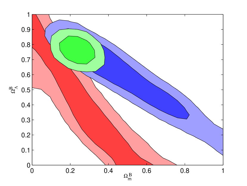
Figure 6: Comparison of the $\Omega_{m}^{\rm B}-\Omega_{\Lambda}^{\rm B}$ Bianchi degeneracy (shaded with 1 and 2$\sigma$ contours) with the familiar CMB geometric degeneracy from WMAP first (blue) and third year + polarisation (green) data (with 1 and 2$\sigma$ contours).

Before continuing it is worth discussing in some detail the effect of each parameter on the structure and scale of the Bianchi templates. The morphology is most sensitive to $\Omega_{m}^{\rm B}$ and $h$, which determine the ‘focus’ and ‘tightness’ (also to some degree the amplitude) of the spiral, respectively. The introduction of dark energy in the form of a cosmological constant energy density creates a correlation between the matter density as the repulsive nature of the former de-focuses the spiral. This degeneracy is almost exact, being broken only by the overall amplitude. Unfortunately, many other parameters can influence the amplitude of the CMB anisotropies on this scale such as the amplitude of primordial scalar (and tensor) density perturbations, the optical depth to reionisation, the spectral ‘tilt’ of the primordial perturbations and of course the Bianchi vorticity $\omega$. This profusion of possible (and mostly degenerate) explanations for the CMB amplitude on large scales make constraints difficult to obtain. Given these difficulties we feel it is justified to fix the cosmological parameters at their WMAP 3-year best fit values (Spergel et al., 2003) varying only the scalar amplitude $A_{s}$. Moreover, careful choice needs to be made over the priors placed on the Euler angles particularly as large regions of the ILC maps contain residual Galactic noise and other emission. In this light we believe a reasonable restriction on the position ($\alpha$ and $\beta$) of the centre of the pattern is well motivated, while leaving the orientation angle ($\gamma$) free to rotate the spiral. Parameter constraints with and without $\Omega_{\Lambda}^{\rm B}$ (models C and F) are shown in Figs 7 and 8 for a left-handed Bianchi component. The angular ranges used, $\alpha=[0.4,1.0]$ and $\beta=[0.1,0.7]$ do implicitly place a prior on the centre of the feature being at least partially associated with the ‘cold spot’ in the southern hemisphere located at roughly $\alpha=0.7$, $\beta=0.4$. Right-handed models examined were entirely unconstrained by the data (see Fig. 9) with a typical best fit $\ln$ likelihood at least 2 units below left-handed models, substantiating the claim in Jaffe et al. (2006) that the only viable Bianchi fit is left-handed. The degenerate effect of $\Omega_{\Lambda}^{\rm B}$ is clearly evident in the laxer constraints, and since we are now only assessing the feature as a non-physical effect there is no benefit in retaining the parameter –it provides no additional effect on the template structure. The above constraints provide robust confirmation of a template very similar to that found by (Jaffe et al., 2005a).

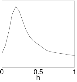
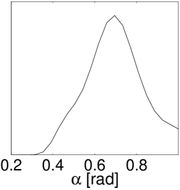
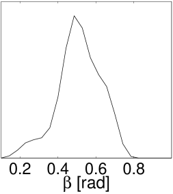
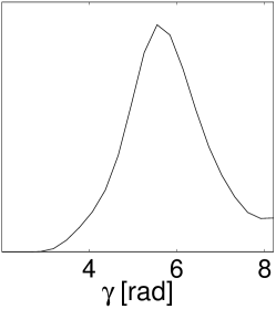
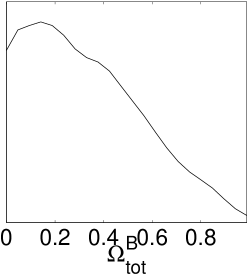
Figure 7: Extracted Bianchi ${\rm VII_{h}}$ parameters including $\Omega_{\Lambda}^{\rm B}$ (left handed model C) from WMAP 3-year data.

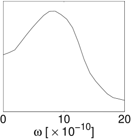
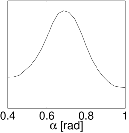
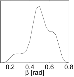
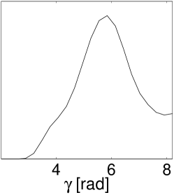
Figure 8: Extracted Bianchi ${\rm VII_{h}}$ parameters with a prior of $\Omega_{\Lambda}^{\rm B}=0$ (left handed model F) from WMAP 3-year data.

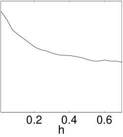
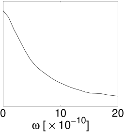
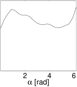
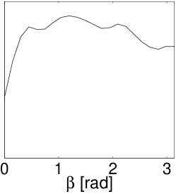
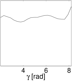
Figure 9: Extracted Bianchi ${\rm VII_{h}}$ parameters with a prior of $\Omega_{\Lambda}^{\rm B}=0$ (right handed model B) from WMAP 3-year data.

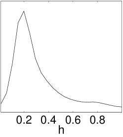
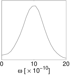
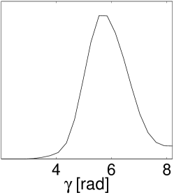
Figure 10: Extracted Bianchi ${\rm VII_{h}}$ parameters with a prior of $\Omega_{\Lambda}^{\rm B}=0$ and centered on the ‘cold spot’ (left handed model G) from WMAP 3-year data. The only model considered which yields a positive evidence.

5.2 Model Selection

The conclusion that the Bianchi ${\rm VII_{h}}$ models may only be treated as templates does not preclude a consideration of the necessity of such a template to explain the data. Indeed, removal of areas of non-Gaussianity and correction of large-scale power would explain serious anomalies in the current data, but at the cost of removal of universal isotropy. The Bayesian evidence provides an ideal way to assess quantitatively whether such action is necessary. As with the previous section we shall assess a template both with and without a dark energy density and with a range of priors on the two positional Euler angles via models B – G. All model comparisons are depicted via $\ln$ evidence differences; $\ln_{\rm A}-\ln_{\rm B-G}$ so that a positive value illustrates a preference for the inclusion of the Bianchi component and vice versa.

Table 4: $\ln$ evidence differences using one and three year all sky maps ILC maps for L and R handed models including a dark energy density.

Data $\backslash$ Model	B (L)	B(R)	C(L)	C (R)	D (L)	D (R)
3-year ILC	-0.9$\pm$ 0.2	-1.4 $\pm$ 0.2	-0.6 $\pm$ 0.2	-1.2 $\pm$ 0.2	+1.2 $\pm$ 0.2	-1.0 $\pm$ 0.2
1-year ILC	-0.9$\pm$ 0.2	-1.5 $\pm$ 0.2	-0.5 $\pm$ 0.2	-1.1 $\pm$ 0.2	+1.2 $\pm$ 0.2	-1.0 $\pm$ 0.2
Data $\backslash$ Model	E (L)	E(R)	F(L)	F (R)	G (L)	G (R)
3-year ILC	-0.9$\pm$ 0.2	-1.3 $\pm$ 0.2	-0.6 $\pm$ 0.2	-1.1 $\pm$ 0.2	+1.1 $\pm$ 0.2	-1.0 $\pm$ 0.2
1-year ILC	-0.8$\pm$ 0.2	-1.5 $\pm$ 0.2	-0.7 $\pm$ 0.2	-1.1 $\pm$ 0.2	+0.9 $\pm$ 0.2	-1.0 $\pm$ 0.2

In agreement with the parameter constraints, little evidence exists for any of the right-handed models, typically at least 1 $\ln$ evidence unit lower than for the left-handed models. We found the results were relatively insensitive to the choice of priors on the energy densities, $h$ and $\omega$, but heavily dependant on the Euler angles. The only preferred model (a marginally significant $\ln$ evidence difference $>$ 1) was found by restricting the pattern to lie centred at the ‘cold-spot’ (models D and G), parameter constraints are shown in Fig. 10. It must be noted that the Bayesian evidence is a prior dependent quantity, so that in general a smaller prior will tend to lift the evidence and vice versa, thus an increased detection using these restricted priors is understandable. However, by still allowing the pattern to rotate freely, via $\gamma$ we still gain all the degrees of freedom necessary to allow the data to decide the best morphology. Indeed all we are saying with this prior is that we believe the ‘cold-spot’ to be driving any detection. The effect of increasing the parameter space with the addition of $\Omega_{\Lambda}^{\rm B}$ is clealy offset by the large volumes of high likelihood that exist along the degeneracy, leaving the evidences almost unchanged. The conclusions are essentially independent on going from 1 to 3 year data, presumably as both maps are effectively cosmic variance limited up to at least $l<10$ where the majority of Bianchi structure lies.

6 Conclusions

We have investigated the possibility of signatures of universal shear and vorticity in 1 and 3-year WMAP data. We implemented Bianchi ${\rm VII_{h}}$ simulations in a fully Bayesian MCMC analysis to extract the best fitting parameters . of the model and to determine whether its inclusion is warranted by the data. We only make a marginally significant detection for a left-handed Bianchi template with parameters; $\Omega_{tot}=0.43\pm 0.04$, $h=0.32^{+0.02}_{-0.13}$, $\omega=9.7^{+1.5}_{-1.6}\times 10^{-10}$ with orientation $\gamma={337^{\circ}}^{+17}_{-21}$) if we restrict its position on the sky to lie centred on the ‘cold-spot’ at ($\alpha=42^{\circ}$,$\beta=32^{\circ}$) –all other models are essentially disfavoured by the data in both 1 and 3 year maps. Since the open universal geometry implied by these templates effectively rules out the Bianchi ${\rm VII_{h}}$ models as the origin of this structure we can only treat these models as template fittings, morphologically similar to some as yet unknown physical cause. Nevertheless our analysis demonstrated that there are interesting effects on large scales yet to be explained in the WMAP data.

Appendix A Bianchi ${\rm VII_{h}}$ templates

We illustrate here our best fitting Bianchi $\rm VII_{h}$ templates found from 3 year WMAP data.

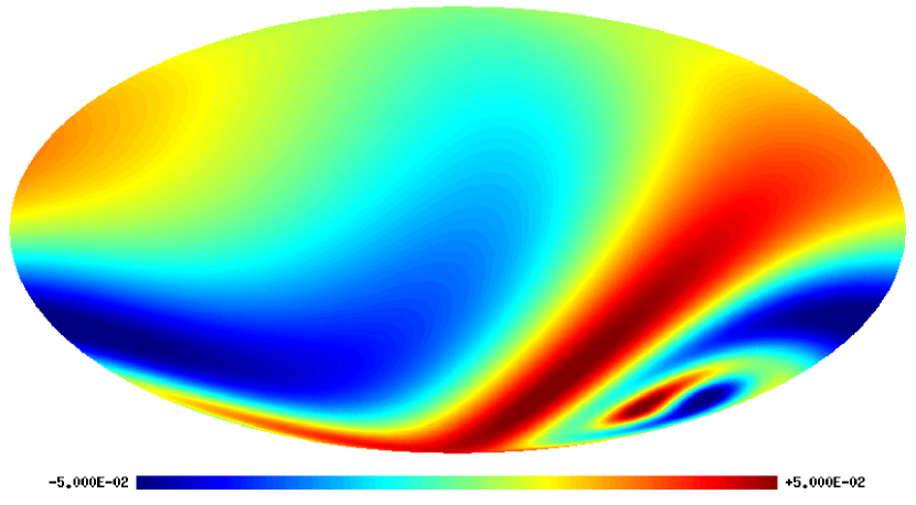
Figure 11: Best fit bianchi template from WMAP 3 year data with parameters $\Omega_{tot}=0.43\pm 0.04$, $h=0.32^{+0.02}_{-0.13}$, $\omega=9.7^{+1.6}_{-1.5}\times 10^{-10}$ with orientation $\gamma={337^{\circ}}^{+17}_{-23}$) and position ($42^{\circ}$, $32^{\circ}$) in Euler angles.

References

- Barrow et al. (1985) Barrow J.D., Juszkiewicz R., Sonoda, D.H., 1985, MNRAS, 213, 917
- Basset et al. (2004) Basset B.A., Corasaniti P.S., Kunz, M., Astrophys. J. Lett., 2004, 617, L1
- Beltran et al. (2005) Beltran M., Garcia-Bellido J., Lesgourgues J., Liddle A., Slosar A., 2005, Phys. Rev. D, 71, 063532
- Bennett et al. (2003) Bennett C.L. et al. 2003, ApJS, 148, 97
- Bridges et al. (2005) Bridges M., Lasenby A.N., Hobson, M.P., in press MNRAS (astro-ph/0502469)
- Cruz et al. (2005) Cruz M., Martinez-Gonzalez E., Vielva P., Cayon L., MNRAS, 356, 29
- Drell et al. (2000) Drell P.S., Loredo T.J., Wasserman, I., Astrophys. J., 2000, 530, 593
- Efstathiou (2004) Efstathiou G., MNRAS, 356, 29
- Eriksen et al. (2004) Eriksen H.K., Banday A.J., Gorski K.M., Lilje P.B., 2004, ApJ, 612, 633
- Gelman & Rubin (1992) Gelman A., Rubin D., Statistical Science, 1992, 7, 457
- Hinshaw et al. (2006) Hinshaw, G. et al., 2006, submitted to ApJ
- Jaffe (1996) Jaffe A., 1996, Astrophys. J., 471, 24
- Jaffe et al. (2005a) Jaffe T.R., Banday A.J., Eriksen H.K., Gorski K.M., Hansen F.K., 2005a, ApJ, 629, L1-L4
- Jaffe et al. (2005b) Jaffe T.R., Hervik, S., Banday A.J., Gorski K.M., 2005b, ApJ, 644, 701-708
- Jaffe et al. (2006) Jaffe T.R., Banday A.J., Eriksen H.K., Gorski K.M., Hansen F.K., 2006, ApJ, 644, 701-708
- Jeffreys (1961) Jeffreys H., 1961, Theory of Probability, 3rd ed., Oxford University Press
- John & Narlikar (2002) John M.V., Narlikar J.V., 2002, Phys. Rev. D, 65, 043506
- Lewis & Bridle (2002) Lewis A. and Bridle S., 2002, Phys. Rev. D, 66, 103511
- Marshall et al. (2003) Marshall P.J., Hobson M.P., Slosar A., 2003, MNRAS, 346, 489
- McEwen et al. (2005) McEwen, J.D, Hobson, M.P., Lasenby, A.N., Mortlock, D.J., MNRAS, 369, 1858-1868
- McEwen et al. (2006) McEwen, J.D, Hobson, M.P., Lasenby, A.N., Mortlock, D.J., MNRAS, 371, L50-L54
- Mukherjee et al. (2005) Mukherjee, P. Parkinson D. Liddle, A., 2005, ApJ, 638, L51
- Niarchou et al. (2004) Niarchou A., Jaffe A., Pogosian L., 2004, Phys. Rev. D, 69, 063515
- de Oliveira-Costa et al. (2003) de Oliveira-Costa A., Tegmark M., Zaldarriaga M., Hamilton A., 2004, Phys. Rev. D, 69, 063516
- Parkinson et al. (2006) Parkinson D., Mukherjee P., Liddle A.R., Phys. Rev. D, 73, 123523
- Saini et al. (2004) Saini T.D., Weller J., Bridle S.L., 2004, MNRAS, 348, 603
- Skilling (2004) Skilling J., 2004, ‘Nested Sampling for General Bayesian Computation’, http://www.inference.phy.cam.ac.uk/bayesys
- Slosar et al. (2003) Slosar A. et al., 2003, MNRAS, 341, L29
- Spergel et al. (2003) Spergel D.N. et al., 2003, Astrophys. J. Suppl., 148, 175
- Stolyarov et al. (2005) Stolyarov, V., Hobson, M.P., Lasenby, A.N., Barreiro, R.B., 2005, MNRAS, 357, 145
- Tegmark et al. (2003) Tegmark M., de Oliveira-Costa A., Hamilton A., 2003, Phys. Rev. D, 68, 123523
- Trotta (2005) Trotta R., 2005, astro-ph/0504022
- Vielva et al. (2005) Vielva P., Martinez-Gonzalez E., Barreiro R., B., Sanz J., L., Cayon L., 2004, ApJ, 609, 22