Time-Delay Measurement for the Quadruple Lens RX J1131$-$1231

Abstract

We have measured the three time delays for the quadruple gravitational lens RX J1131$-$1231 using two seasons of monitoring data. The short delays between cusp images are A–B = $11.98^{+1.52}_{-1.27}$ days and A–C = $9.61^{+1.97}_{-1.57}$ days. The long A–D delay for the counter image is not as precisely determined because of the season gaps, but the data suggest a delay of $-87\pm 8$ days. The short delays are difficult to explain using standard isothermal halo models of the lensing potential, which instead prefer A–B and A–C delays of $\sim 1$ day for reasonable values of the Hubble constant. Matching the cusp delays is possible by adding a significant ($\sim 5\times 10^{10}$ M_☉) amount of matter nearly coincident ($\sim 0\farcs 05$ South-East) with the A image. Adding such a satellite also helps improve the quasar and lens astrometry of the model, reduces the velocity dispersion of the main lens and shifts it closer to the Fundamental Plane. This is suggestive of a satellite galaxy to the primary lens, but its expected luminosity and proximity to both image A and the system’s bright Einstein ring make visual identification impossible even with the existing HST data. We also find evidence for significant structure along the line of sight toward the lens. Archival Chandra observations show two nearby regions of extended X-ray emission, each with bolometric X-ray luminosities of 2-3 $\times$ $10^{43}$ ergs s^-1. The brighter region is located $\Delta\theta\approx$ 153″ from the lens and centered on a $z=0.1$ foreground cD galaxy, and the fainter and presumably more distant region is 4-5 times closer (in angular separation) to the lens and likely corresponds to the weaker of two galaxy red sequences (which includes the lens galaxy) previously detected at optical wavelengths.

1. Introduction

Gravitationally lensed quasars are useful tools for studying the matter distribution of intermediate redshift ($0.1\lesssim z\lesssim 1.0$) galaxies. Robust estimates of the total (luminous plus dark) lensing mass usually follows from just measuring the image positions. However, quantifying the presence of halo substructure, constraining the mass profile’s radial distribution, or parsing the relative contributions from stars and dark matter requires additional information. For example, the flux ratios of lensed images are sensitive to the presence of halo substructure (e.g., Metcalf & Zhao 2002) and the incidence of so-called “anomalous” ratios at radio wavelengths is consistent with CDM predictions that a few percent of the halo mass should be left in satellites (Dalal & Kochanek, 2002). At optical wavelengths, interpreting such anomalies in light of stellar microlensing implies that $\lesssim 25\%$ of the surface mass density at the image locations must be in a smooth (non-stellar) form (Schechter & Wambsganss, 2002; Keeton et al., 2006).

Another key observation is time delays. The time delays between lensed images measure a combination of the Hubble constant and the surface mass density $\langle\kappa\rangle=\langle\Sigma\rangle/\Sigma_{c}$ of the lens at the radius of the lensed images, with $H_{\rm o}\propto(1-\langle\kappa\rangle)$ to lowest order (Kochanek, 2002). For the six simple time delay lenses that we have at present, Kochanek (2002) noted that four (PG1115+080, Schechter et al. 1997, Barkana 1997, Impey et al. 1998; SBS1520+530, Burud et al. 2002b; B1600+434, Burud et al. 2000, Koopmans et al. 2000; and HE2149–2745, Burud et al. 2002a) yield $H_{\rm o}$ predictions consistent with the HST Key Project result of 72 km s^-1 Mpc^-1 (Freedman et al., 2001) only if the lensing galaxies have constant $M/L$ profiles (that is, declining rotation curves at the system’s Einstein radius). The remaining two systems (HE1104–1805, Ofek & Maoz 2003; HE0435–1223, Kochanek et al. 2006) have measured delays consistent with the Key Project only with mass profiles that drop off slower than isothermal (that is, rising rotation curves at the locations of the lensed images). In the case of HE0435–1223, the best-fit model yields an average mass convergence at the system’s Einstein radius that is 20% larger ($\langle\kappa\rangle\simeq 0.6\pm 0.05$) than expected for an isothermal halo. Taken at face value, the range in $\langle\kappa\rangle$ estimates imply a heterogeneous mix of mass profiles for lensing galaxies, with the likely explanation that we are seeing the effects of the lensing environment. Lens galaxies located at the center of their respective groups will naturally have an extended dark matter halo (yielding flat or rising rotation curves), while lens galaxies located in the field or group periphery will have mass distributions dominated by their stellar components (falling rotation curves). Under this interpretation, it becomes important to not only expand the sample of systems with measured time-delays in order to sample as wide a range of environments as possible, but also to characterize the lensing environment for systems with measured delays as thoroughly as possible.

In this paper, we present our time-delay measurements and explore the lensing environment for the quadruple lens RX J1131$-$1231 (hereafter J1131). Our original motivation was to use the measured delays and assumed $H_{\rm o}$ to estimate the lens surface mass density at the J1131 image positions. Coupled with the robust total mass estimate obtained from the image separations and the measured luminosity distribution of the lens obtained from HST/NICMOS data, this would allow us to estimate the radial mass profile of the lens and separate the luminous and dark contributions to the total lensing mass (as done recently for HE 0435–1223; Kochanek et al. 2006). Unfortunately, the measurement of unexpected delays for this system makes such an approach unfeasible. Instead, we simply focus on constructing a plausible macromodel that can reproduce the delays while assuming an isothermal halo for the main lens.

This system was originally identified as a ROSAT X-ray source and subsequently revealed to be a quadruply-imaged quasar by Sluse et al. (2003). The lensing geometry consists of a background $z_{s}=0.658$ quasar lensed by a foreground $z_{l}=0.295$ elliptical galaxy, and there is a prominent Einstein ring evident even in ground-based optical data. Sluse et al. (2003) also detected variability on the order of 0.3 magnitudes from the total integrated system flux over an eight month baseline. Overall, the system’s demonstrated variability, wide image separation (A to D separation of 3$\farcs$2), prominent lens galaxy and quad plus ring morphology made J1131 an attractive target for long-term monitoring and followup studies. In §2 and §3 we describe our monitoring program and time-delay measurements and comment on the microlensing variability observed in the system over the course of the campaign. High-resolution HST/ACS and NICMOS images of the lens and immediate environment are described in §4, and evidence for at least two clusters along the line of sight are presented using far IR (§5) and X-ray (§6) observations obtained with the Spitzer and Chandra Space Telescopes. We then explore several iterations of parametric and non-parametric lens models and discuss their implications in §7. In summary, we find it difficult to simultaneously explain the system geometry and measured time delays using a single profile for the main lens galaxy, but find it possible if a significant amount of substructure is present near one of the cusp images. Finally, we summarize our results and describe avenues for future work on this system in §8.

2. Lens Monitoring

The monitoring data for J1131 were obtained as part of the ongoing program described by Kochanek et al. (2006); details of the reduction pipeline and lens fitting procedures can also be found in that reference. Briefly, we monitor approximately 25 lensed quasars at cadences of 1-2 times per week, with typical observations of three 2-5 minute exposures per epoch in either Sloan $r$ or Johnson $R$. Each lens is assigned up to 5 nearby reference stars which serve as local flux calibrators and as shape templates for the analytic PSF model. Point sources are modeled as a combination of three elliptical Gaussians and extended objects (lens galaxies) are modeled using Gaussian approximations to de Vaucouleurs profiles (which allows for rapid analytic convolutions with the seeing disc). The relative astrometry for each system is fixed using observations from the CASTLES HST program, and relative photometry for the system images are obtained by minimizing $\chi^{2}$ residuals between the data and analytic model.

The monitoring data for J1131 were obtained using the queue-scheduled SMARTS/CTIO 1.3m telescope in the Southern Hemisphere and the MDM 2.4m, WIYN 3.5m, and APO 3.5m telescopes in the Northern Hemisphere. The bulk (94%) of data were taken with the SMARTS 1.3m using the dual-beam optical/IR ANDICAM camera (DePoy et al., 2003) and covering the 2003-2004 and 2004-2005 seasons for a total of 101 epochs. These observations consisted of three 5 minute $R$-band exposures and six 2.5 minute $J$-band exposures at each epoch. The IR data are considerably less sensitive than the optical data and we focus only on the $R$-band light curves here. Additional observations include three Sloan $r$-band epochs consisting of 1.5-2 minute exposures using the SPIcam CCD on the APO 3.5m, two $R$-band epochs of 2-3 minute exposures using the WTTM camera on the WIYN 3.5m, and two $R$-band epochs of 3 minute exposures using the 8K Mosaic CCD on the MDM 2.4m. The APO, WIYN and MDM light curves were calibrated by interpolating the quasar and reference star data points onto the respective SMARTS curves, yielding star offsets of $-0.01$, $0.00$ and $-0.02$ mags and quasar offsets of $0.08$, $-0.02$ and $0.04$ mags, respectively. We only kept data with seeing better than 1$\farcs$7 FWHM, or about half the maximum image separation.

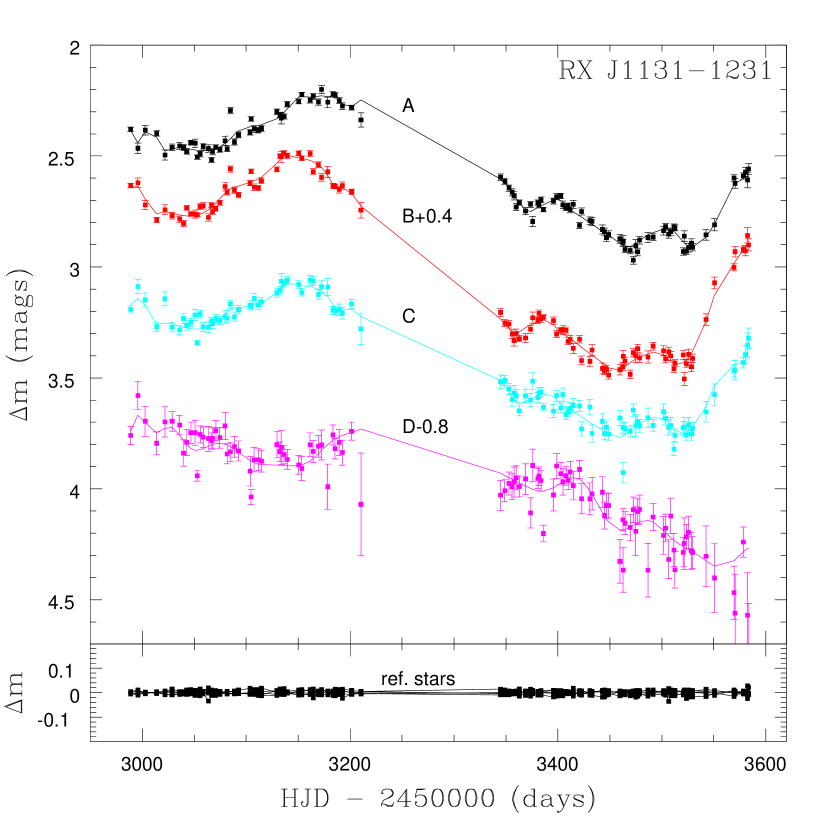
Figure 1.— Light curves for images A–D. The B and D curves are offset for clarity. The best fit models are for $N_{\rm src}=30$, $N_{\mu}=4$ for each separate season for images $A$, $B$ and $C$, and for $N_{\rm src}=40$, $N_{\mu}=3$ for the joint seasons for image D. Differential photometry for 5 nearby reference stars is shown in the bottom panel.

Figure 1 shows the four quasar light curves and Table LABEL:tab:lcurve gives the quasar magnitudes and reference star differential variability at each epoch. Over the two seasons, each image varied by as much as 0.7 mag. Significant correlated variability on timescales of weeks is also apparent for the three brighter images.

3. Time Delays Measurements

The light curves are modeled as a sum of two Legendre polynomial series. The first series, of order $N_{\rm{src}}$, models the intrinsic source variability of the quasar and is the same for all four quasars images up to a time delay shift for each pair. The second series, of order $N_{\mu}$, is different for each image and models the different macrolensing magnifications ($0^{th}$ order) and the uncorrelated microlensing variability for each quasar image ($1^{st}$ order and above). Exact prescriptions for the fitting forms can be found in Kochanek et al. (2006). The merit function for each light curve is minimized by differentiating with respect to the polynomial coefficients and solving the resulting linear set of equations, which yields estimates for the time delays between each image, a lightcurve for the intrinsic source variability, and the relative microlensing lightcurves for three of the four images.

Figure 2.— Overlapping curves for images A (open squares), B (triangles) and C (filled squares) after shifting by the best-fit time delay and removing the macromodel magnification and microlensing variability from images B and C. The much noisier D curve is not shown. Errorbars are suppressed for clarity.

The A, B and C images show relative delays of about 1-2 weeks, much shorter than the length of each observing season. Since all the signal when solving for the ABC delays will come from same-season data, we fit the two season’s ABC light curves simultaneously (that is, we solve for a single set of time delays constrained by both seasons) but model each season’s lightcurve separately. (We discuss modeling the D curve below). The $F$-test is used to decide when further increases in $N_{\rm{src}}$ and $N_{\mu}$ do not yield improvements to the fits. We find that most of the source-curve improvements occur up to $N_{\rm{src}}=10$, beyond which the higher source-curve complexity does not significantly improve $\chi^{2}$. Significant improvement in the microlensing model occurs from $N_{\mu}=0$ (macromodel magnifications only and no microlensing) to $N_{\mu}=4$, arguing for microlensing variations that are somewhat more complex than just a simple linear trend (which would be described by $N_{\mu}=1$). We adopt $N_{\rm{src}}=30$, $N_{\mu}=4$ as our standard model for the A, B and C images, where the larger source curve order should lead to conservative uncertainties in the delay estimates. This model gives A–B, A–C and B–C delays of $11.98^{+1.52}_{-1.27}$  $9.61^{+1.97}_{-1.57}$ and $-2.20^{+1.55}_{-1.64}$ days (1$\sigma$), respectively. As a check on the results, we also fitted each season’s light curve as a stand-alone dataset using a separate code that uses brute-force (Powell) minimization, and we find delays consistent with the quoted error bars. Figure 2 shows the ABC light curves after shifting by the relative delays and subtracting the microlensing and macromodel magnifications, leaving just the source variability observed in each image.

Fitting for image D’s light curve is less precise. In addition to the lower signal-to-noise, D is expected to lag the other images by $\sim 100$ days (Sluse et al., 2003), which would shift about half of D’s data points into the season gaps of the other images. This leaves less overlapping data to measure a delay, but we can improve the available signal by modeling the two seasons as one continuous light curve. Fixing the relative ABC delays at the values determined above, we use a $N_{\rm{src}}=40$, $N_{\mu}=3$ model to obtain an A–D delay of $-87\pm 8$ days ($1\sigma$). The reported best-fit is driven by aligning the broad valley in image D at MJD $\approx$ 3125 days with the similar valley in the ABC curves at MJD $\approx$ 3040, with most of the season two drop in D’s brightness shifted into the ABC season gap. If this feature is not correctly matched, then the absence of other distinguishing features in the D curve would mean that the A–D delay is unconstrained with the extant data. If the feature is correctly matched, then the D delay is measured to an accuracy of about 10%.

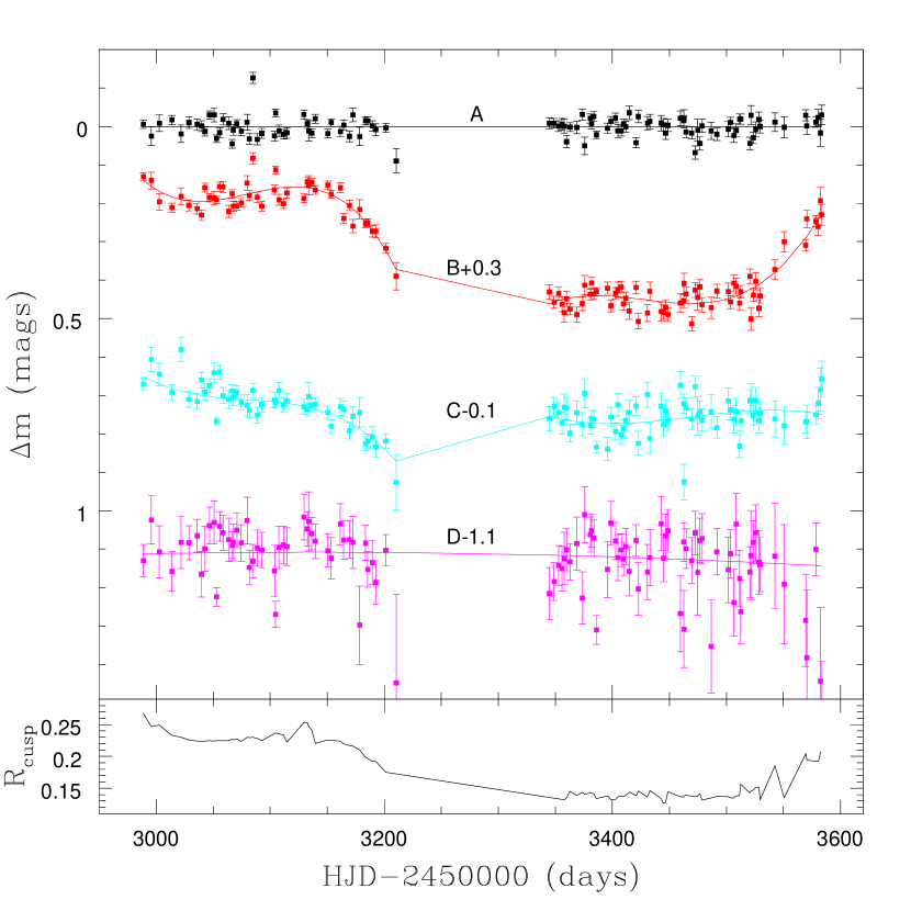
Figure 3.— (Top): The microlensing light curves for RX J1131$-$1231. Shown are the light curves for images A–D after subtracting the time-delay shifted A model curve as a model for the source variability. (Bottom): $R_{\rm cusp}$ for images A, B and C formed using the best-fit curves in Figure 1 after shifting by the respective time delays.

Figure 3 shows the residual microlensing light curves after subtracting the appropriately time-delay shifted source variability (arbitrarily set to be image A’s light curve) from each quasar image. Both B and C show a drop in brightness relative to A toward the end of the first season, and image B shows a rapid rise in brightness at the end of the second season. Image D does not show significant variability apart from a gradual ($\Delta m\simeq 0.05$ mag) decline during both seasons, although the lower signal to noise complicates the analysis.

It is likely that image A is responsible for the first season drop seen in the B and C curves since we only measure the differential effects. This would imply a net increase in A’s brightness by $\sim$0.2 mag due to microlensing toward the end of the first season. The differences between the B and C microlensing light curves are evidence for a similar amount of microlensing in one or both of these images as well. For example, B’s upswing at the end of season two is not seen in image C. Also, image B spends most of season two $\sim$0.2 mag fainter than its season one average, while image C maintains more or less the same average flux from one season to the next.

One succinct way to quantify the effects of microlensing is to look at the lensing cusp relation (Mao & Schneider, 1998), which states that the sum of the signed image magnifications is zero for the triplet of images formed when a source is near a cusp caustic (images A, B and C for J1131). The relation can be phrased in terms of the observed image fluxes ($F_{A},F_{B},F_{C}$) by dividing through by the unknown source flux, yielding $R_{\rm cusp}=|F_{A}+F_{B}+F_{C}|/(|F_{A}|+|F_{B}|+|F_{C}|)$. While the cusp relation for a source asymptotically close to a cusp has $R_{\rm cusp}=0$, in practice $R_{\rm cusp}$ as defined will increase by several tenths as the source is placed farther from the cusp, not to mention the additional perturbing effects of micro- and millilensing (Keeton et al., 2003, hereafter KGP). For a system configuration such as J1131, one can place a strong upper limit on the baseline $R_{\rm cusp}$ value (before micro- or millilensing perturbations, that is, assuming a perfectly smooth potential model) of $\lesssim$0.1 (KGP). This value is significantly lower than the $R_{\rm cusp}\approx 0.35\pm 0.03$ measured from the Sluse et al. (2003) $V$-band discovery data, and lead KGP to classify J1131 as a “cusp-anomaly” system.

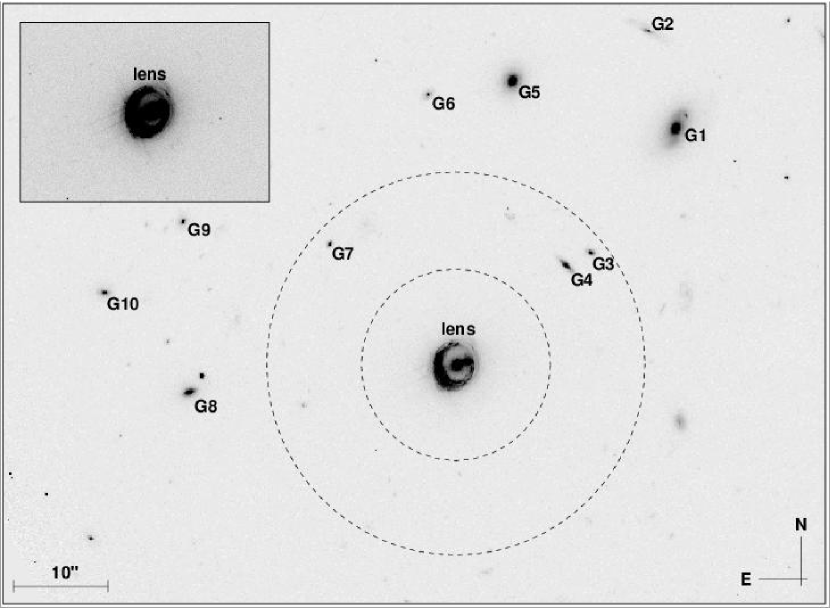
Figure 4.— PyDrizzled HST/ACS $I$-band image of RX J1131$-$1231 and the surrounding field. Prominent nearby galaxies are labeled. Concentric circles mark the 10″ and 20″ radii centered on the lens galaxy. The inset shows the inner 10″ region at the same scale but at 10$\times$ higher contrast.

Anomalous $R_{\rm cusp}$ values indicate the presence of substructure in the lens galaxy, but it can not discern whether the anomaly is due to microlensing by stars or due to millilensing by substructure (either dark matter clumps or luminous satellites). However, only microlensing can change $R_{\rm cusp}$ on observable timescales, so tracking changes in $R_{\rm cusp}$ tracks the microlensing contributions. The bottom panel of Figure 3 shows $R_{\rm cusp}$ computed using the time-delay corrected light curves (shifting to the image A time frame). $R_{\rm cusp}$ is $\sim$0.23 during most of the first season but begins to drop, becoming less “anomalous” with respect to the KGP estimate toward the season gap. At the same time, B and C drop in brightness and the $R_{\rm cusp}$ value remains at $\sim$0.14 for the bulk of the second season. The resolved Chandra X-ray observations of J1131 reported by Blackburne et al. (2005) have $R_{\rm cusp}=0.75\pm 0.05$ on MJD = 3108 due to the significantly dimmed flux of component A (see their Figure 1a). Taken together, the SMARTS and Chandra data suggest that the saddlepoint A image was in a demagnified microlensing state for much of season one and varied closer to the unperturbed macromodel magnification heading into season two.

The HST observations of J1131 described in the next section yield respective $R_{\rm cusp}$ values in the V, I and H filters of $0.26\pm 0.06$, $0.17\pm 0.05$ and $0.08\pm 0.01$. Assuming the baseline $R_{\rm cusp}$ value of $\lesssim 0.1$ (KGP), the trend with wavelength agrees with the notion that microlensing preferentially affects smaller emission regions of the quasar accretion disk (under the assumption that longer wavelengths correspond to lower disk temperatures, which then correspond to larger radii from the central black hole). However, it is important to remember that the cusp anomaly may be due to the presence of substructure on scales comparable to the image separations. For example, models with a satellite galaxy near one of the cusp images (explored in §7.3) predict an $R_{\rm cusp}$ value of about 0.5 even before any microlensing effects. In such a case, the offsets from $R_{\rm cusp}\lesssim 0.1$ cannot be interpreted as strictly a sign of microlensing, but the variations in $R_{\rm cusp}$ seen in time and across wavelength still point to abundant microlensing for J1131.  

4. HST Observations

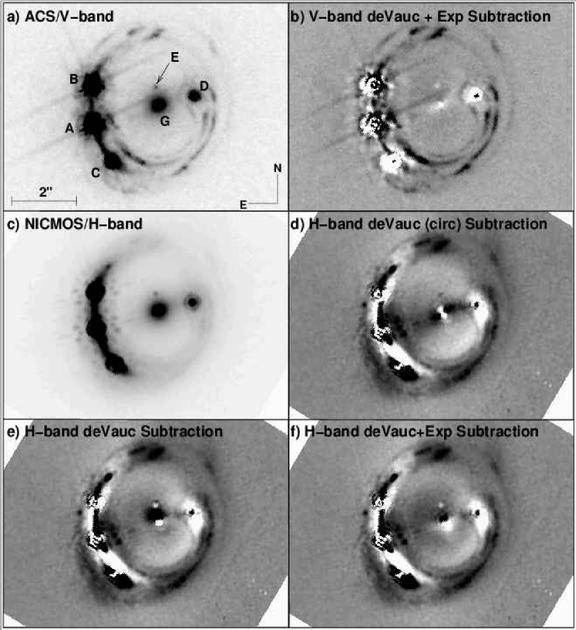
Figure 5.— Combined HST images of RX J1131$-$1231. (a): ACS/$V$-band image. (b): Same as (a), but after subtracting the best-fit point source, lens galaxy and ring model. (c): NICMOS/$H$-band image. (d): Same as (c), but after subtracting the best-fit point source, lens galaxy and ring model. Contrast in both residual panels stretches from $-7\%$ to $+7\%$ of the respective peak lens galaxy flux.

High-resolution images of J1131 were obtained with the ACS/Wide Field Camera (WFC; Ford et al. 1998) and NICMOS detectors on board the HST as part of the CASTLES imaging program (PID 9744). Both of these public data sets have also been recently analyzed by Claeskens et al. (2006), and we make comparisons between the separate reductions below. The optical ACS images were taken with the F814W ($I$-band) and F555W ($V$-band) filters on 22 and 24 June 2004, respectively. Exposures were 33 minutes through each filter using a 5-point dither pattern. The data were reduced using the IRAF/CALACS package as part of the “on-the-fly” reprocessing at the time of download. Subsequent cosmic-ray rejection, geometric correction, and image combinations were performed using the standard PyRAF programs available for ACS data reduction. The infrared NICMOS images were taken with the NIC2 camera and F160W ($H$-band) filter on 17 November 2003, and consisted of two sets of four-point dither MULTIACCUM exposures for a total on-source integration of about 89 minutes. The NICMOS data were reduced using the NICRED software described in Lehár et al. (2000).

Figure 4 shows a 1′ field of view surrounding J1131 from the stacked $I$-band data. The environment within 10″ of the lens is devoid of galaxies, and the nearest galaxies to the lens (G3, G4 and G7) are 15-20″ distant. The Figure 4 inset shows the inner 10″ region centered on J1131 at 10$\times$ higher contrast to emphasize the lack of nearby structure. The nearest galaxies with comparable magnitudes to the lens are G1 and G5, roughly 30″ distant toward the North-North-West.

In Figures 5a and 5c we show the $V$- and $H$-band closeup images of J1131. A complex pattern of lensed knots from the quasar host galaxy is present, presumably because the relatively low redshift host galaxy is a star-forming spiral galaxy. There is also a faint fifth object, component E in Figure 5 (denoted component X in Claeskens et al. 2006), roughly 0$\farcs$5 North of the lens galaxy. The object shows a clear Airy ring in the $H$-band data, so it is unresolved.

To model the light distribution, we first tried fitting the $H$-band data using a seven component model: five point-sources for images A-E, a de Vaucouleurs profile for the lens galaxy, and a lensed de Vaucouleurs profile for the quasar host galaxy to model the continuous portion of the Einstein ring emission. For the fitting, we used the IMFIT package written by B. McLeod (see, e.g., Lehár et al. 2000). The lensing potential was modeled as a singular isothermal sphere plus external shear using just the $H$-band image positions as constraints for the purpose of mapping the host galaxy onto the image plane. We also tried exponential and Gaussian profiles for the quasar host, but the de Vaucouleurs profile yielded the lowest residuals. Figure 5d shows the residuals after fitting a circularly symmetric de Vaucouleurs profile for the lens galaxy and reveals the lens to be elongated roughly along the A-D line. Allowing an elliptical de Vaucouleurs profile for the lens does well at modeling the galaxy ellipticity (Figure 5e) but still leaves extended residuals near the center of the lens with a peak flux of about 12% of the unsubtracted galaxy peak flux. To model this extra emission, we added an exponential profile centered on the de Vaucouleurs model. This addition did a better job at accounting for the bulk of the extra emission, although there are systematic residuals in the core of the lens galaxy ($\sim$10% of the unsubtracted galaxy flux; Figure 5f) that are suggestive of a slightly misaligned center for the de Vaucouleurs and exponential profiles.

The inability to model the main lens with a single profile was noted by Claeskens et al. (2006) as well. The two-component galaxy model naturally suggests a disk+bulge morphology, except that we find the de Vaucouleurs model to be a better fit to the elongated structure than to the bulge. For an S0 galaxy, one would expect the opposite, namely an exponential disk and a de Vaucouleurs bulge. We tried to coax the models to assign the exponential profile to the disk by using judicious choices for the initial conditions, but the models consistently preferred a de Vaucouleurs disk and exponential bulge. The de Vaucouleurs component of the galaxy model is best characterized by an effective radius $R_{e}=1\farcs 58\pm 0\farcs 29$, axis ratio of $0.51\pm 0.02$, and major axis orientation of $-62\arcdeg\pm 2\arcdeg$. The exponential component of the galaxy has a best-fit scale length of 0$\farcs$20 $\pm$ 0.01, axis ratio of 0.79 $\pm$ 0.04, and major axis orientation 33° $\pm$ 4°.

For the $V$- and $I$-band data, we fixed the astrometric and structural components of the system at the values from the $H$-band eight component model and solved for the relative photometry. Table LABEL:tab:astromphot lists the results for all three filters. The relative positions for the A, B and C images agree within the quoted errorbars with the Claeskens et al. (2006) positions, but we do find a small offset of 0$\farcs$009 (3$\sigma$) for the D image and a much larger offset of 0$\farcs$029 (15$\sigma$) for the main galaxy position. The lens offset between the two reductions is about half an ACS pixel and may originate with the different light profiles used when modeling the main lens galaxy (de Vaucouleurs + Exponential for our fit, single Sersic profile for the Claeskens et al. 2006 fit).

The colors of the system components are plotted in Figure 6. Components A and B are three-quarters of a magnitude redder in $I-H$ compared to C and D, but all have nearly identical $V-I$ colors. Component E is significantly redder by about $1.5$ mag in $V-I$ than the other four quasar images. The reddening vector assuming a $R_{V}=3.1$ Galactic extinction law is given by the arrow in Figure 6, and shows that E is unlikely a reddened copy of a fifth quasar image. Its $I-H$ color is too red by several tenths of a magnitude for a late-K/early-M dwarf as well. Its color is consistent with the primary lens galaxy, and Claeskens et al. (2006) suggested that $E$ may be an unresolved satellite galaxy.

The main lens galaxy has total (exponential + de Vaucouleurs) colors in $V-I$ and $I-H$ of $1.84\pm 0.11$ and $1.83\pm 0.20$, respectively. These are bluer by $\sim$0.2 magnitudes than expected for a $z_{f}=2.5$ burst galaxy model observed at $z\approx 0.3$ (see Figure 6), but the difference is not unreasonable compared to the spread in galaxy colors observed in other lensed systems at similar redshifts (Rusin et al., 2003). As for the exponential contribution to the galaxy model, its magnitude is fainter than the de Vaucouleurs component by 2.1 mags, 1.5 mags and 1.2 mags in the $V$, $I$ and $H$ filters, respectively. Its colors are redder than the de Vaucouleurs component, as expected for a bulge-like component to the lens galaxy. However, as already noted, the morphology is not as expected for a true bulge and the spatial offset between the “bulge” and “disk” components evident in Figure 5e is puzzling.

Figure 6.— Colors for RX J1131$-$1231 system components A-E and lens galaxy components Gd (de Vaucouleurs component) and Ge (exponential component). Color tracks for the dwarf main sequence (heavy line) and a $z_{f}=2.5$ burst galaxy model (thin line) are also drawn. The arrow gives the reddening magnitude and direction assuming a $R_{V}=3.1$ Galactic extinction law and wavelength-dependent parameters from Cardelli et al. (1989).

5. Spitzer Observations

We also observed J1131 with the Infrared Array Camera (IRAC) on board the Spitzer Space Telescope on 11 June 2005. Observations consisted of a 36-point dither pattern for each of the four IRAC bandpasses (3.6, 4.5, 5.8, and 8 $\mu m$), covering an area of roughly 7$\farcm$5 $\times$ 7$\farcm$5 centered on the lens. The data received from the Spitzer Science Center had passed through the standard IRAC pipeline (consisting of flat-field corrections, dark subtraction, and linearity and flux calibrations) and the resulting Basic Calibrated Data (BCD) files served as our input for MOPEX drizzling. The BCD images were combined using a final scale of 0$\farcs$863 pixel^-1, and Figure 7 shows the [3.6] image of J1131 and surrounding field.

Even after drizzling onto the finer pixel grid, the J1131 A-D separation spanned only four pixels. The lack of spatial resolution complicates any analysis of the lens components and we instead focused on the IR colors of field galaxies. After identifying extended sources in the field using the SExtractor package (Bertin & Arnouts, 1996, ver. 2.2.2), we searched for red sequences (e.g., Gladders & Yee 2000) in the IR color-magnitude diagrams indicative of overdense regions of elliptical and S0 galaxies (groups or clusters). The resulting CMDs were suggestive of a low-redshift ($z<0.3$) overdensity of galaxies with [3.6]-[4.5] colors of $\sim 0.1$, but the concentration was not defined enough to estimate a redshift. Since the Spitzer observations were obtained, Williams et al. (2005) have indeed identified two red sequences for the J1131 field using deep $VRI$ observations obtained with the KPNO Mayall 4m and CTIO Blanco 4m telescopes (see their Figure 8). The dominant red sequence has a centroid (denoted by the eastern bullseye in Figure 7) located 2$\farcm$1 East of J1131 G and $\approx$45″ to the South-South-West from a bright elliptical galaxy identified in the mid-infrared images (G0 in Figure 7). Galaxy G0 is suggestive of a cD galaxy associated with the primary Williams et al. (2005) red sequence, implying significant structure along the line of sight toward J1131 (additional evidence supporting this claim is presented using the archival X-ray observations described below). The second, weaker red sequence detected by Williams et al. (2005) has a flux-weighted centroid 25″ North-West of J1131 G (western bullseye in Figure 7) and includes the lens galaxy itself.

6. Chandra Observations

Given the evidence for structure along the line of sight, we re-analyzed the archival 10 ks Chandra observation of J1131 (see Blackburne et al. 2005) taken on 12 April 2004 using the ACIS-S3 detector, with the goal of identifying X-ray emission from halos associated with the Williams et al. (2005) red sequences. The smoothed X-ray emission (after excising the X-ray flux associated with the lensed quasar) is shown as contours on top of the IRAC [3.6] image in Figure 7. We identified two extended sources of X-rays in the field aside from the lens flux analyzed by Blackburne et al. (2005). The first is the bright emission centered 153″ North-East of J1131 (at 11^h32^m1$\fs$4, $-12$° 31′ 6″  J2000; centroid accuracy of approximately 2″). The X-ray position is coincident with the large elliptical galaxy (G0) identified in the mid-infrared images and within an arcminute of the red sequence flux centroid identified by Williams et al. (2005). This galaxy (and two others within three arcminutes) has a redshift measured from the Las Campanas Redshift Survey of $z=0.10$ and the region was identified as an optically-selected group by Tucker et al. (2000). Thus, the red sequence, the cD galaxy and the extended X-ray emission confirm the presence of a foreground cluster at $z=0.1$.

We extracted the ACIS spectrum of the extended emission and used XSPEC (Arnaud, 1996) to fit it with a thermal plasma model modified by Galactic absorption and obtained a good fit to the data with a $\chi^{2}=22$ for 41 degrees of freedom. We estimated an unabsorbed 0.4-8 keV flux of $(7.5\pm 0.8)\times 10^{-13}$ ergs cm^-2 s^-1, a bolometric X-ray luminosity of $(3.1\pm 0.5)\times 10^{43}$ ergs s^-1 assuming the cluster is at $z=0.1$, and a temperature of $1.13\pm 0.03$ keV. The temperature and luminosity are roughly consistent with typical $L$-$T$ relations (e.g., Wu et al. 1999; Helsdon & Ponman 2000; Xue & Wu 2000; Rosati et al. 2002) for groups and clusters, providing further confirmation of the cluster redshift.

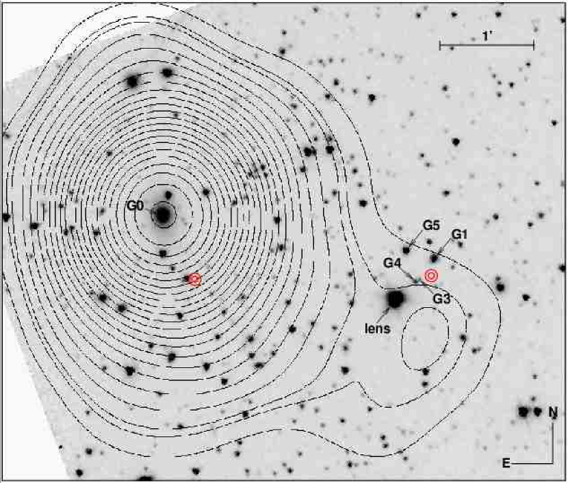
Figure 7.— Smoothed X-ray contours plotted on top of the IRAC Channel 1 (3.6 $\mu$m) image. X-ray contours are logarithmic except for the first two contour levels, which mark the $2\sigma$ and $3\sigma$ confidence levels. The eastern (western) bullseye marks the raw centroid of the primary (secondary) galaxy red sequence detected by Williams et al. (2005).

The second extended source of X-ray emission is South-West of the lens, but it is fainter and the analysis is complicated by other point sources in the field. To proceed, we did a general search for faint extended emission following the procedures used in Dai & Kochanek (2005). We used the CIAO tool wavdetect to identify point sources in the ACIS-S3 field and then replaced them with nearby background regions to create a soft band (0.5-2 keV) image. We smoothed this image with a Gaussian of width $\sigma=25$″ to find a source 33″ Southwest of the lens (11^h31^m50$\fs$1, $-12$° 32′ 23″, J2000). Because of the low ($\sim 3\sigma$) significance of the detection and the effects of masking the overlapping emission from the lens, the position uncertainty is comparable to the smoothing scale. Since this flux overlaps the lens and is close to the centroid of the weaker red galaxy sequence detected by Williams et al. 2005 (western bullseye in Figure 7), we tentatively identify the emission as from the lens group at redshift of $z_{l}=0.295$. The measured count rate in the 0.5-2 keV band is 0.004 cts s^-1 within a circle of radius 25″, corresponding to an unabsorbed flux of $1.7\times 10^{-14}$ ergs cm^-2 s^-1. If we use a $\beta$ model to extrapolate the X-ray flux to a larger aperture and assume a temperature of $T\simeq 1.5$ keV, then we estimate that the bolometric luminosity of this second cluster is $2\times 10^{43}$ ergs s^-1. Thus, the halo associated with the lens group is comparable in bolometric luminosity to the halo associated with the low redshift group, but would require 10$\times$ the integration time to characterize at the same signal-to-noise.

7. Lens Models and Interpretations

In this section, we describe our mass modeling efforts aimed at reproducing the HST geometry and the SMARTS time delays. We discuss three model variations. First, we look at both isothermal and variable-slope power-law halo models for the main lens galaxy (§7.1), but in general find that such models cannot explain the long ($\sim$ 10 days) A–B and A–C time delays. Next, we try a non-parametric mass model of the system (§7.2). In general, such models add no information beyond that available in parametric models, but the asymmetric mass reconstruction suggests a satellite galaxy or other substructure near image A may be required to explain the anomalous delays. Finally, we return to parametric models (§7.3) consisting of the primary isothermal halo for the main lens and a secondary halo for the presumed substructure near image A. Such models can plausibly reproduce both the long A delays and the image astrometry at the expense of consuming the remaining degrees of freedom.

7.1. Basic Isothermal Models

We first tried to model J1131 using the standard singular isothermal ellipsoid embedded in an external shear (Kassiola & Kovner, 1993; Kormann et al., 1994). For constraints, we used the HST/ACS $H$-band positions (Table LABEL:tab:astromphot) with error bars of 3 mas for the quasar positions and the three SMARTS time delays. We looked at three model sequences: model SISx uses a spherical halo centered on the lens galaxy plus an external shear; model SIEx allows for halo ellipticity plus shear; and model SIEx+ allows the halo center to move with respect to the galaxy center but constrained with errorbars of 5 mas. The astrometry and time delays give 13 constraints, so the models have 6, 4 and 4 degrees of freedom, respectively. We ignored the flux ratios. All models were minimized in the image-plane using the gravlens software of Keeton (2001) and adopting a $(\Omega_{m},\Omega_{\Lambda})=(0.3,0.7)$, $H_{\rm o}=70$ km s^-1 Mpc^-1 cosmology. The model results are summarized in Table LABEL:tab:models.

Figure 8.— Schematic of RXJ1131$-$1231 environment. Labels X-ray 1 and 2 denote the large and small X-ray emissions detected in the Chandra observations, and Red Seq. 1 and 2 denote the two red sequence centroids identified by Williams et al. (2005); the dashed lines marks the 1$\sigma$ spread in the external shear direction for the SIEx+ model; the pentagons mark the locations of neighboring galaxies identified in the HST/ACS data. The diameter of the X-ray 2 circle is the X-ray smoothing scale of 25″. Symbol sizes for the galaxies are proportional to the square root of their ACS $I$-band fluxes. The lens galaxy $I$-band flux (not depicted by symbol size) is nearly twice that of G1.

None of the models gives a statistically acceptable fit to the observations; the best-fit SIEx+ model has a final $\chi^{2}$/dof of 74.1/4. The simpler SISx and SIEx models cannot reproduce the image astrometry, with rms values between the observed and predicted quasar locations of 33 and 13 mas, respectively (final $\chi^{2}$/dof values of 538/6 and 138/4, with more than half of the $\chi^{2}$ budget coming from the quasar positions). The SIEx+ model fits the quasar positions essentially perfectly (image rms of 2 mas) at the expense of shifting the halo center by 12 mas ($4\sigma$) from the measured luminous galaxy position. The situation is worse if we use the Claeskens et al. (2006) image and galaxy positions, which yield $\chi^{2}$/dof values of 534/6, 158/4, and 130/4 for the SISx, SIEx and SIEx+ models, respectively. A substantial external shear is also required for both the Table LABEL:tab:astromphot and Claeskens et al. (2006) positions – greater than 10% for all models – and points at $-83$° East of North for the SIEx+ case (where the convention is for the shear direction to point towards or away from the perturber.) There is no obvious perturber along the shear direction (see Figure 8); a galaxy with roughly the same velocity dispersion as the lens would produce a 10% shear at 9″, but the nearest galaxies of significance (G3 and G4) are 20″ away and at the wrong position angle. Galaxy G8 lies at the correct position angle, but is much too distant to produce a 10% shear given its brightnesses and that of the main lens galaxy (see Figure 4). The shear does not point toward either of the X-ray halos detected in the Chandra data, or toward either of the red sequence centroids identified by Williams et al. (2005). This likely indicates that either there is no single external perturber dominating the shear or that the external shear is attempting to compensate for an inadequacy in the main lens model.

The more troublesome problem is that all models fail to reproduce the measured time delays. The SIEx+ profile predicts A–B and A–C delays of 0.98 and 1.23 days (assuming $H_{\rm o}$ = 70 km s^-1 Mpc^-1) compared to the measured values of roughly 12 and 10 days. Formally these are 9$\sigma$ and 5$\sigma$ discrepancies. Note that the predicted B–C delay of 0.25 days for the SIEx+ model agrees within 2$\sigma$ with the measured value of $-2.20^{+1.55}_{-1.64}$ days, so the problem is chiefly with the A image. The situation cannot be corrected by simply rescaling $H_{\rm o}$, since matching the A–B and A–C delays would require an unrealistic Hubble constant of $\approx$ 10 km s^-1 Mpc^-1.

The long A delay is difficult to explain. There are many examples of model perturbations leading to systematic uncertainties in time delay predictions (see Schechter 2005 for a review), but these typically alter the delay predictions at the 10% level and not the factor of 10 needed here. For example, the mass-sheet degeneracy (Gorenstein et al., 1988) rescales the image delays by $\Delta\tau\propto(1-\langle\kappa\rangle)$ by superimposing a mass-sheet of surface density $\langle\kappa\rangle$. One might expect a convergence of $\langle\kappa\rangle\simeq 0.1$-$0.3$ from matter associated with the nearby X-ray halos (e.g., as with systems Q0957+561, Barkana et al. 1999; RXJ 0911+0554, Burud et al. 1998), but this would uniformly shorten all delays by 10%-30%, and not preferentially lengthen the A delay. To a similar degree, small variations in the radial exponent of the halo density profile ($\sim$ 10%) alter delay predictions by a comparable fraction (Kochanek, 2002), again of insufficient magnitude to explain the A delay. An example of an extreme change in the density slope is to use a de Vaucouleurs constant mass-to-light ratio model with an effective radius matching the value measured from the NICMOS data. Such a model can match the astrometry as well as the SIEx+ model provided the de Vaucouleurs center is allowed to float, but the predicted cusp delays are still $\sim 1$ day.

Abandoning the assumption of isothermality, we also explored a range of elliptical power-law profiles with three-dimensional density profiles falling as shallow as $1/r$ to as steep as $1/r^{4}$. We found that highly elliptical profiles steeper than $1/r^{3}$ could produce long cusp delays provided the halo was orientated along the A-G line. Because of the high ellipticity, such models concentrated more mass near A than near B and C, increasing the Shapiro contribution to the A delay. However, the required ellipticity to produce an A–B delay of even half the observed value was flatter than $e=0.9$. Such a mass distribution would indicate a prominent disk galaxy, and this is clearly inconsistent with the morphology of the lens observed in the NICMOS data.

7.2. Non-Parametric Models

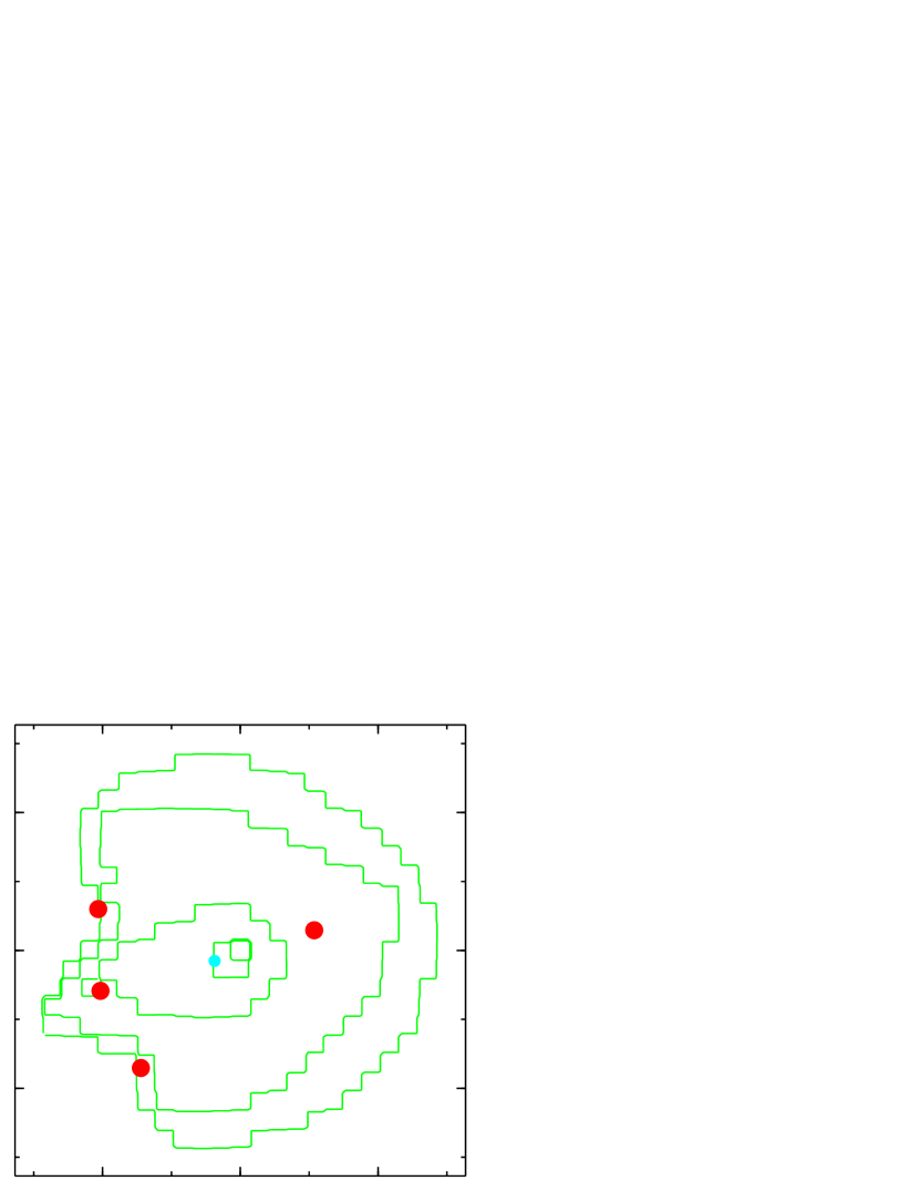
Figure 9.— PixeLens ensemble-average mass map of RX J1131$-$1231, as constrained by the system astrometry and ABC time delays. The mass contours are logarithmically spaced at factors of 2.5 in surface density, beginning with the outer contour at $\kappa\approx 0.16$.

Lacking a successful macromodel, we turned to non-parametric models using the PixeLens software of Saha & Williams (2004). As noted above, such models do not add any more information than present in parametric models since they are grossly underconstrained, but they may indicate where the parametric models are qualitatively wrong. PixeLens works by reconstructing a pixelated mass map of the lens using the image positions and time delays as constraints. For J1131, we reconstructed both symmetric and asymmetric mass models over a 6″ $\times$ 6″ grid centered on the lens with a “pixrad” of 11, yielding around 530 separate mass elements. Since PixeLens assumes negligible errors for all input values, we tried models both with and without the more uncertain D delay but found little qualitative change in the final mass map.

The reconstruction for the asymmetric mass distribution is shown in Figure 9. (For the symmetric reconstruction, the eastern half of the structure is mirror-imaged on the western half, producing an unrealistic four-leaf clover mass distribution). There is a clear protrusion surrounding image A. PixeLens’s solution for increasing the A delay is to have significant variation in the angular distribution of matter along the three cusp images by increasing the surface mass density around image A ($\kappa\simeq 0.9$) as compared to the surface mass densities at images B and C ($\kappa\simeq 0.1$-$0.2$). Qualitatively, this is similar to our result found for a highly elliptical disk-like halo overlapping the A image. However, the asymmetric reconstruction stresses that what is chiefly needed is a higher surface mass density at A compared to the other two cusp images, suggesting that a satellite galaxy or other undetected substructure at this location may be responsible for the anomalous delay.

7.3. Substructure Near Image A

There is no visual sign of a satellite galaxy near image A in the HST images or the corresponding subtraction residuals. A red satellite galaxy would be most evident in the F160W image, but the significant Einstein ring emission and PSF residuals complicates any visual search near the lensed images. To explore if a perturber could reproduce the cusp delays, we added an SIS mass model over a grid of positions surrounding image A and looked at how each model adjusted for the J1131 time delays. The main lens galaxy was again modeled using the SIEx+ profile, and we fitted both the astrometric and delay constraints as before. We found that a perturber with an Einstein radius of $\sim 0\farcs 2$ and placed within $\sim 0\farcs 1$ South-East of the A image could lengthen the A–B and A–C delays by several days, but such models consistently formed two additional images of the background quasar. The perturber’s proximity to image A means that its critical curve always maps into a source-plane caustic near the source position, creating a six-image region inside the primary lens astroid caustic. While one of these extra images is always highly demagnified and located at the perturber position, the other typically forms at twice the perturber-A separation with a magnification $\sim 10\%$ that of image A. Such an image would be easily identified in the HST data.

We can avoid the formation of extra images by adding a core radius $s$ to the perturber’s profile, such that the projected density is given by

$$\kappa(r)=\frac{b^{\prime}}{2}\frac{1}{\sqrt{s^{2}+r^{2}}}$$ (1)

(e.g., Kassiola & Kovner 1993; Kormann et al. 1994). The exact criteria needed to prevent extra images depend on the perturber’s core size and mass scale. Consider a model where the main lens (modeled as an SIE) and perturber (modeled as a softened isothermal sphere, or IS) are colinear along the x-axis with the main lens at the origin and the perturber at a distance $x=x^{\prime}$. Including an external shear term (with shear angle $\theta_{\gamma}$ measured from the x-axis), the potential $\phi(x)$ is

$$\phi(x)=\phi_{\rm SIE}(x)+\phi_{\rm IS}(x-x^{\prime})+\frac{\gamma x^{2}}{2}\cos(2\theta_{\gamma}).$$ (2)

The appearance of extra images first becomes possible (that is, a critical line and corresponding six-image caustic are first formed) when a solution to the lens equation exists at $x=x^{\prime}$. This translates into a condition on the potential of

$$\frac{\partial^{2}\phi}{\partial x^{2}}\arrowvert_{x=x^{\prime}}=1,$$ (3)

or, after substitution,

$$\frac{b^{\prime}}{2s}\approx 1,$$ (4)

where we have neglected a shear term that is always much smaller than unity for reasonable models. No extra images are possible when $b^{\prime}/2s\lesssim 1$ and multiple images are possible (provided the source is inside the six-image caustic) otherwise.

Figure 10.— Optimal perturber positions for the best-fit sub-critical ($b=1.4s,b=1.6s,b=1.8s$), critical ($b=2.0s$) and super-critical ($b=2.1s,b=2.2s$) models. The three contours outline the $\Delta\chi^{2}=2.6,4.3,6.2$ ($1\sigma$, $2\sigma$, and 3$\sigma$ for two parameters) contour parameters for the critical case. The location of image A is marked. For scale, the dotted box shows the size of one ACS pixel centered on image A.

Figure 11.— Goodness of fit for two super-critical ($b=2.2s$ and $b=2.1s$), critical ($b=2.0s$) and sub-critical ($b=1.8s$) perturbers near image A. Minimums for the $b=1.6s$ and $b=1.4s$ cases are also noted by the two tick marks.

We looked at a range of perturber models: two super-critical ($b=2.2s$ and $b=2.1s$), a critical ($b=2.0s$) and three sub-critical ($b=1.8s$, $b=1.6s$ and $b=1.4s$). During the minimization, a large penalty term was added to the merit function whenever the source position crossed into the six-region caustic, insuring that only four-image models were accepted. We also constrained the orientation of the main lens halo using the measured NICMOS position and associated error, which helped stabilize the ellipticity of the primary lens. This approach gave a final tally of 12 parameters (two for the source position, seven for the main lens, and three for the perturber) and 14 constraints for two degrees of freedom. Table LABEL:tab:models summarizes the result for the critical perturber.

Figure 10 shows the optimal perturber positions for the model sequence and the confidence contours for the critical ($b=2.0s$) case. For all models, the perturber position was tightly constrained to a region between $0\farcs 03$ to 0$\farcs$11 South-East of image A. In Figure 11, we show the resulting $\chi^{2}/dof$ for each model as the perturber’s core radius is increased from $s=0$″ (the singular case) to $s=0\farcs 3$ (about 1.3 kpc at the lens redshift). Note that for the two super-critical models, $\chi^{2}$ rapidly increases once a threshold core radius is crossed, with roughly 90% of the increase coming from the quasar positions. The abrupt increase is due to the growing size of the six-image caustic as the perturber’s core radius and potential depth are increased, which displaces the source position from its optimal location inside the six-image region. This means a super-critical perturber is highly unlikely since it requires a fine-tuned source position in order to match the quasar astrometry while remaining outside the six-image region. The critical and sub-critical models avoid the formation of the six-image caustic and consequentially show no abrupt increase in $\chi^{2}$.

As seen from Figure 11, the critical model is marginally preferred over the sub-critical cases. There are two notable improvements for the optimal critical model compared to the single halo model considered in §7.1. First, both the quasars and galaxy astrometry are now fitted essentially perfectly: $\chi^{2}/dof$ = 0.3/2 compared to 13/4 for the SIEx+ case, with virtually all (99%) of the $\chi^{2}$ budget now coming from the time delays. Second, the cusp delays are lengthened considerably: A–B, A–C and A–D delays of 5.90, 7.88 and $-80$ days, respectively. The remaining model parameters are quite reasonable as well, with a nearly round main lens galaxy (ellipticity of 0.14) and small external shear (4%). Thus, it is possible to improve both the overall astrometry and the time delay predictions by adding a perturber halo nearly coincident with image A, provided the halo is soft enough to avoid the formation of extra images.

The A–B delay is still a factor of two smaller than measured (a 4$\sigma$ discrepancy). Since the Shapiro contribution to the time delays depends on differences in effective potential between images, one simple way to fine-tune the delays is to vary the radial slope of the perturber. With a variable slope $\alpha$, the projected surface density $\kappa(r)$ can be written as

$$\kappa(r)=\frac{1}{2}\frac{b^{\prime 2-\alpha}}{({s^{2}+r^{2}})^{1-\alpha/2}},$$ (5)

where again $s$ is the core radius and the normalization is chosen such that $b$ is the system’s Einstein radius in the limit of an isothermal profile ($\alpha\rightarrow 1$) and vanishing core radius. For small core radii, the effective potential is approximately given by $\phi(r)\approx b^{\prime 2-\alpha}r^{\alpha}/\alpha^{2}$. Generating longer A–B and A–C delays requires a larger difference in the A–B and A–C effective potentials, which is possible for steeper than isothermal ($\alpha<1$) mass profiles.

To test if a non-isothermal slope could more closely match the delays, we allowed the potential depth $b^{\prime}$ and halo slope $\alpha$ to vary independently while again looking at a range of core radii $s$. This modification consumes the remaining two degrees of freedom and we expect a perfect fit for a plausible model. Indeed, we found that a halo slope with $\alpha=0.7$-$0.8$ could reproduce both the astrometry and measured time delays essentially perfectly although with a clear degeneracy between the size of the core radius and the halo slope. For the $s=0\farcs 2$ model (summarized in Table LABEL:tab:models), the predicted delays were 12.0, 13.8 and -85 days for A–B, A–C and A–D, respectively, with an overall $\chi^{2}/dof$ of 4.7/0. It is interesting that we still find $\chi^{2}>0$ even for zero degrees of freedom. The only $\chi^{2}$ contribution for all $s\gtrsim 0\farcs 15$ models is from the A–C delay, although it is more instructive to look at the discrepancy using the B–C difference. The predicted B–C delays (between +1.0 and +1.8 days for the range of core radii considered) is in the opposite sense of the measured value ($-2.20^{+1.55}_{-1.64}$ days). The delay ordering among images is a model-independent feature of a lens (e.g., Saha & Williams 2003), so if the sense of the delay is measured incorrectly then even a model with zero degrees of freedom will be unable to reproduce the incorrect delay sense. All models considered in this paper predict B trailing C (B–C $>0$), implying that images A and B are the “merging” image pair normally seen in inclined-quad configurations and that the overall image ordering is CBAD. Therefore, if the measured C delay is off by 2-3 $\sigma$ such that the measured B–C delay becomes positive, then it might explain the non-zero $\chi^{2}$.

Figure 12.— Potential strength ($b^{\prime}$) and halo slope ($\alpha$) for a non-isothermal perturber. The dotted line marks the potential strength for the just-critical perturber, using each model’s core radius and best-fit halo slope.

Figure 12 shows the degeneracy between the perturber slope $\alpha$ and core radii $s$, as all models in the figure yield $\chi^{2}/dof$ values between 3/0 and 5/0. We also plot the best-fit potential depth $b^{\prime}$ for the perturber and the condition for the just-critical case (dotted line), which for the power-law profile is

$$\frac{1}{2}\left(\frac{b^{\prime}}{s}\right)^{2-\alpha}\approx 1.$$ (6)

The total $\chi^{2}/dof$ gradually drops from $4.7/0$ at $s=0\farcs 15$ to $3.0/0$ at $s=0\farcs 45$ with again the only significant contribution coming from the C delay. Over this range, $b^{\prime}$ if fairly constant, ranging from 0$\farcs$25 to 0$\farcs$28, and the halo slope increases from $\alpha$ = 0.7 to 0.8. Note that for $s\gtrsim 0\farcs 15$, the perturber no longer sits on the just-critical line as seen for the optimal ($b=2s$) isothermal model. Thus a steeper-than-isothermal profile not only reproduces the long A delay but also naturally avoids the formation of extra images.

7.4. Mass of the Perturber

The cylindrical mass for the surface density given in Eq. 5 increases as $M_{\rm cyl}(r)\propto r^{\alpha}$, so formally the total perturber mass in the adopted model is unbounded. Adopting a cut radius comparable to the A-C or A-B image separations ($\approx$1$\farcs$2, or 5.3 kpc at the lens redshift) gives an enclosed perturber mass of $4.7\times 10^{10}$ M_☉. As a comparison, the mass enclosed by the primary lens galaxy out to the same cylindrical radius (centered on its respective profile) is $4.4\times 10^{11}$ M_☉, so the perturber has $\lesssim 10\%$ of the mass of the main lens at comparable radii. This is fairly significant and one might expect some visual evidence if it is indeed a satellite galaxy. We can estimate a plausible luminosity to the perturber by scaling its velocity dispersion with that of the main lens and using the Faber & Jackson (1976) relationship. For an enclosed mass that scales with velocity dispersion as $M(R)\propto\sigma^{2}$, the factor of 10 difference in mass translates into a factor of 3.2 in velocity dispersion, or a factor of 100 difference in luminosity assuming $L\propto\sigma^{4}$. Such a galaxy would be extremely difficult to see given the ring emission and light from image A, even after image subtraction. For example, scaling from the observed count-rate of the main lens measured in the NICMOS image, the predicted peak count rate from the perturber is only $\sim$0.008 cnts s^-1. The rms count rate within a 0$\farcs$4 radius around image A after subtracting the quasar images and ring emission (Figure 5f) is 0.058 cnts s^-1, which is larger than the peak signal expected from the satellite galaxy by a factor of seven. Thus even if the perturber were a bona fide satellite galaxy, it is doubtful we would detect it in the existing HST images.

7.5. Placement on the Fundamental Plane

One check on the models is to compare the predicted velocity dispersion of the main lens galaxy with the value expected from the Fundamental Plane (FP; Djorgovski & Davis 1987; Dressler 1987). Almost all lens galaxies lie on the present-day FP provided one allows for passive luminosity evolution with redshift (Treu et al., 2001, 2002; Rusin et al., 2003). When studying gravitational lenses, it is convenient to phrase this evolution in terms of the galaxy’s $B$-band mass-to-light ratio $(M/L)_{B}$ measured inside the system’s Einstein radius (see Treu et al. 2001 for a thorough discussion). Parameterizing to first-order in redshift as $\Delta\log(M/L)_{B}=az$, studies of gravitational lens galaxies find values between $a\approx 0.5$ (Rusin et al., 2003) and $a\approx 0.7$ (Treu et al., 2005). Similar results are found for cluster (van Dokkum et al., 1998) and field (van Dokkum et al., 2001) galaxies out to $z\approx 0.8$ that are not associated with lensing.

Figure 13.— $M/L_{B}$ evolution of the J1131 lens galaxy (arrows offset in redshift for clarity) from the present-day FP, computed using combinations of the total de Vaucouleurs plus Exponential galaxy magnitude, just the de Vaucouleurs component magnitude, and the two velocity dispersion estimates described in the text. The other 18 points are evolutions obtained for lens galaxies listed in Rusin et al. (2003) that have spectroscopically measured lens redshifts. The solid lines denote the best-fit Rusin et al. (2003) slope of $\Delta\log(M/L)=-0.54\pm 0.04$ using 28 gravitational lens galaxies.

Using a $z_{f}=2.5$ starburst SED to calculate the necessary $k$-corrections and evolution effects, the restframe $B$-band surface brightness for J1131 G is 20.62 $\pm$ 0.05 mag arcsec^-2 using the total (de Vaucouleurs plus exponential) galaxy magnitude and 20.83 $\pm$ 0.03 mag arcsec^-2 using just the de Vaucouleurs galaxy magnitude. The system’s velocity dispersion is either 353 $\pm$ 2 km s^-1 or 337 $\pm$ 2 km $s^{-1}$ for the SIEx+ or SIEx+ plus $\alpha=0.72$ perturber model. Both values correspond to extremely bright galaxies, $6L_{*}$ and $5L_{*}$ respectively for $\sigma_{*}=225$ km $s^{-1}$. Such galaxies are rare but not unheard of. The Bernardi et al. (2003a) SDSS sample of $\sim$9000 field ellipticals contains galaxies with velocity dispersions as large as 400 km s^-1. Although a $\sigma=350$ km s^-1 galaxy is 200 times less common than a $\sigma\approx 170$ km s^-1 galaxy found at the peak of the elliptical velocity dispersion function (Sheth et al., 2003), the cross-section for lensing scales as $\sigma^{4}$ so massive galaxies are preferentially favored. Finally, the galaxy intermediate-axis effective radius measured from the NICMOS data gives a physical size of $R_{e}=5.0\pm 1.2$ kpc.

The evolution rates required to place J1131 G onto the present-day FP are plotted in Figure 13. Four estimates are computed, using the possible combinations of the two surface brightness estimates and the two velocity dispersion estimates. Also plotted are rates computed for 18 other gravitational lenses with measured lens and source redshifts listed in Rusin et al. (2003). Contrary to the Rusin et al. (2003) sample of lens galaxies, all J1131 G evolution rates are inconsistent with passive luminosity evolution, with only the halo plus perturber model and total (de Vaucouleurs plus exponential) galaxy magnitude rate consistent with no evolution at all at the 1$\sigma$ level ($a=0.02\pm 0.05$). Another way to view this is that the galaxy’s inferred velocity dispersion is simply too large for its measured luminosity. Adopting $M_{*}=-19.79+5\log(h)\pm 0.04$ (Madgwick et al., 2002), $\gamma=4.0\pm 0.25$ (Bernardi et al., 2003b) and $\sigma_{*}=225\pm 22.5$ km s^-1, the Faber-Jackson relationship yields $\sigma=274\pm 28$ km s^-1 using the combined de Vaucouleurs plus exponential magnitude. This estimate is considerable lower than the value of $\sigma=337\pm 2$ km s^-1 obtained from the halo plus perturber model, suggesting that there may be an additional source of mass contributing convergence inside the Einstein ring besides the main lensing galaxy. Part of the solution likely lies in the mass convergence associated with the overlapping X-ray halos detected in the Chandra data and the unknown object component E, if it is truly a satellite galaxy to the primary lens. Both effects would lower the inferred value of the main lens velocity dispersion by accounting for some of the inferred mass inside the system’s Einstein ring.

8. Summary and Conclusions

We have measured the time delays for the quadruple lens RX J1131$-$1231 based on two seasons of monitoring data from the SMARTS/CTIO 1.3m telescope. The short delays for the cusp images are A–B = $11.98^{+1.52}_{-1.27}$ and A–C = $9.61^{+1.97}_{-1.57}$ and the long delay for the counter image is A–D = $-87\pm 8$. The A–B and A–C delays are an order of magnitude larger than expected using a standard elliptical model of the lens galaxy. One plausible explanation arises from a satellite galaxy or other dark substructure about $0\farcs 05$ from the central cusp image, although some fine-tuning is required to match the observed properties of the system. In particular, for the power-law mass models explored here, the perturber must have a core radius of $\gtrsim 0\farcs 2$ ($\gtrsim$ 1 kpc) to avoid the formation of extra images of the background quasar, a steeper than isothermal mass profile ($\alpha\approx 0.7;\rho\propto r^{-\alpha}$), and a significant total mass within the A-C and A-B image separations of $\sim 4.7\times 10^{10}$ M_☉ (about 10% of the main lens galaxy for comparable radii). Although massive, such a satellite galaxy would have a luminosity only $\sim$1% of the main lens, making it undetectable in the extant data given the perturber’s proximity to the bright quasar A image and the prominent Einstein ring emission.

Ancillary evidence for such a perturber comes from the improved astrometry of the quasar positions and primary lens galaxy. As noted by Claeskens et al. (2006), using a standard isothermal halo for the main lens can reproduce the relative quasar positions but not the position of the lensing galaxy. This was addressed by Claeskens et al. (2006) by adding an $m=4$ octupole term (characteristic of boxy/disky isodensity contours) to the lensing potential, although they admit that the physical nature of the term is difficult to interpret. Comparable deviations from pure elliptical models have been ruled out for four other lens galaxies using the shapes of Einstein rings (Yoo et al., 2005). Here, we have shown that including a perturber near image A allows for an essentially perfect fit to the quasars and galaxy astrometry while simultaneously explaining the anomalous cusp delays.

We have also re-analyzed the Chandra X-ray data first presented by Blackburne et al. (2005) and found evidence for two X-ray halos along the line of sight toward J1131. The brighter halo is coincident with a foreground ($z=0.1$) cD galaxy 2$\farcm$5 North-East of the lens and corresponds to the stronger of two galaxy red sequences detected in the optical by Williams et al. (2005). The fainter halo is much closer to the lens and presumably includes J1131 itself, given the halo’s proximity to the lens and proximity to the weaker of the two galaxy red-sequences identified by Williams et al. (2005).

Overall, the data suggest a very complicated lensing environment for J1131. The lens galaxy is likely part of a $z\approx 0.3$ group or cluster of galaxies with sufficient mass to support a $\sim 1.5$ keV X-ray halo; there is a foreground cluster of galaxies along the line of sight as evidenced by a second X-ray halo of similar temperature and centered on a prominent $z=0.1$ cD galaxy; a significant mass perturbation near the A image is required to explain the anomalous time delays for the cusp images; modeling the surface brightness profile of the main lens requires at least two distinct profile shapes, suggestive of a more complicated primary lens than a simple de Vaucouleurs-shaped elliptical; and finally, there is a faint, point-like object 0$\farcs$5 North of J1131 G with colors similar to those of the main lens galaxy but otherwise of an as-of-yet undetermined nature. These complications make it difficult at present to use the measured time delays to either estimate the Hubble constant or to constrain the overall mass profile of the main lens. The monitoring program has revealed extensive ($\sim$ 0.3-0.4 mag) microlensing variability in the optical on time scales of months, so future microlensing studies of the system are promising.

Progress with future mass modeling will at least require measuring the central velocity dispersion of J1131 G to break the mass-sheet degeneracy between the main lens galaxy and X-ray halos identified in the Chandra data. Such information will likely help to reconcile the lack of apparent $M/L$ evolution for the main lens as well, since it will provide an estimate of the halo convergence inside the Einstein ring that is currently assigned to the lens galaxy. Deep imaging and spectral observations of component E are obviously required as well, but may prove challenging given its overall faintness, extremely red color, and proximity to the main lens.

Table 1Lightcurves for RXJ 1131$-$1231

HJD	$\chi^{2}$/dof	++Comp. A++	++Comp. B++	++Comp. C++	++Comp. D++	++ref. stars++	++Telescope++
$2988.811$	$1.29$	$2.379\pm 0.009$	$2.233\pm 0.009$	$3.192\pm 0.014$	$4.560\pm 0.037$	$\phantom{-}0.006\pm 0.002$	SMARTS
$2995.804$	$5.62$	$2.465\pm 0.010$	$2.220\pm 0.009$	$3.088\pm 0.013$	$4.380\pm 0.027$	$\phantom{-}0.009\pm 0.002$	SMARTS
$3002.819$	$10.58$	$2.383\pm 0.007$	$2.321\pm 0.007$	$3.147\pm 0.009$	$4.495\pm 0.021$	$\phantom{-}0.008\pm 0.002$	SMARTS
$3013.819$	$2.33$	$2.398\pm 0.008$	$2.388\pm 0.008$	$3.270\pm 0.013$	$4.595\pm 0.034$	$\phantom{-}0.007\pm 0.002$	SMARTS
$3021.790$	$6.08$	$2.495\pm 0.009$	$2.342\pm 0.009$	$3.144\pm 0.013$	$4.499\pm 0.028$	$\phantom{-}0.009\pm 0.002$	SMARTS
$3028.765$	$4.21$	$2.460\pm 0.007$	$2.369\pm 0.007$	$3.271\pm 0.010$	$4.496\pm 0.021$	$\phantom{-}0.007\pm 0.002$	SMARTS
$3035.815$	$3.93$	$2.454\pm 0.007$	$2.385\pm 0.007$	$3.284\pm 0.010$	$4.512\pm 0.021$	$\phantom{-}0.007\pm 0.002$	SMARTS
$3039.758$	$2.89$	$2.461\pm 0.008$	$2.404\pm 0.008$	$3.232\pm 0.012$	$4.639\pm 0.035$	$\phantom{-}0.008\pm 0.002$	SMARTS
$3042.783$	$0.76$	$2.479\pm 0.012$	$2.334\pm 0.011$	$3.264\pm 0.021$	$4.591\pm 0.059$	$-0.003\pm 0.002$	SMARTS
$3046.734$	$1.41$	$2.440\pm 0.009$	$2.361\pm 0.009$	$3.249\pm 0.015$	$4.547\pm 0.040$	$\phantom{-}0.004\pm 0.002$	SMARTS
$3050.769$	$7.66$	$2.443\pm 0.007$	$2.361\pm 0.006$	$3.216\pm 0.009$	$4.547\pm 0.020$	$\phantom{-}0.007\pm 0.002$	SMARTS
$3052.918$	$1.50$	$2.505\pm 0.006$	$2.365\pm 0.006$	$3.341\pm 0.008$	$4.740\pm 0.020$	$\phantom{-}0.008\pm 0.002$	APO
$3055.713$	$2.08$	$2.491\pm 0.009$	$2.328\pm 0.008$	$3.213\pm 0.012$	$4.555\pm 0.027$	$\phantom{-}0.008\pm 0.002$	SMARTS
$3058.707$	$4.69$	$2.457\pm 0.007$	$2.324\pm 0.007$	$3.271\pm 0.010$	$4.567\pm 0.021$	$\phantom{-}0.006\pm 0.002$	SMARTS
$3063.712$	$4.85$	$2.466\pm 0.008$	$2.377\pm 0.007$	$3.271\pm 0.011$	$4.574\pm 0.026$	$\phantom{-}0.006\pm 0.002$	SMARTS
$3066.739$	$1.14$	$2.518\pm 0.011$	$2.322\pm 0.010$	$3.243\pm 0.015$	$4.582\pm 0.033$	$\phantom{-}0.008\pm 0.002$	SMARTS
$3067.760$	$3.05$	$2.480\pm 0.008$	$2.350\pm 0.008$	$3.256\pm 0.012$	$4.573\pm 0.028$	$\phantom{-}0.007\pm 0.002$	SMARTS
$3070.686$	$0.99$	$2.460\pm 0.011$	$2.337\pm 0.010$	$3.232\pm 0.018$	$4.538\pm 0.045$	$\phantom{-}0.002\pm 0.002$	SMARTS
$3074.674$	$1.25$	$2.471\pm 0.010$	$2.311\pm 0.010$	$3.241\pm 0.017$	$4.569\pm 0.042$	$\phantom{-}0.003\pm 0.002$	SMARTS
$3079.825$	$17.12$	$2.431\pm 0.005$	$2.237\pm 0.005$	$3.225\pm 0.007$	$4.517\pm 0.015$	$\phantom{-}0.018\pm 0.002$	EIGHTK
$3081.715$	$3.84$	$2.467\pm 0.007$	$2.263\pm 0.007$	$3.230\pm 0.010$	$4.642\pm 0.023$	$\phantom{-}0.008\pm 0.002$	SMARTS
$3084.852$	$13.07$	$2.294\pm 0.004$	$2.158\pm 0.004$	$3.168\pm 0.005$	$4.633\pm 0.012$	$-0.239\pm 0.002$	WTTM
$3088.616$	$3.85$	$2.437\pm 0.007$	$2.254\pm 0.007$	$3.224\pm 0.011$	$4.610\pm 0.024$	$\phantom{-}0.008\pm 0.002$	SMARTS
$3092.574$	$3.52$	$2.405\pm 0.007$	$2.275\pm 0.007$	$3.192\pm 0.010$	$4.629\pm 0.025$	$\phantom{-}0.007\pm 0.002$	SMARTS
$3103.735$	$2.04$	$2.393\pm 0.009$	$2.222\pm 0.008$	$3.173\pm 0.014$	$4.721\pm 0.047$	$\phantom{-}0.004\pm 0.002$	SMARTS
$3104.662$	$6.17$	$2.333\pm 0.004$	$2.168\pm 0.004$	$3.177\pm 0.005$	$4.837\pm 0.014$	$-0.164\pm 0.002$	WTTM
$3107.612$	$4.61$	$2.378\pm 0.007$	$2.241\pm 0.007$	$3.142\pm 0.010$	$4.669\pm 0.025$	$\phantom{-}0.007\pm 0.002$	SMARTS
$3111.596$	$2.37$	$2.383\pm 0.008$	$2.244\pm 0.008$	$3.171\pm 0.012$	$4.669\pm 0.032$	$\phantom{-}0.004\pm 0.002$	SMARTS
$3114.620$	$3.75$	$2.375\pm 0.007$	$2.211\pm 0.007$	$3.157\pm 0.010$	$4.676\pm 0.025$	$\phantom{-}0.007\pm 0.002$	SMARTS
$3129.597$	$1.85$	$2.300\pm 0.009$	$2.160\pm 0.008$	$3.117\pm 0.014$	$4.601\pm 0.044$	$\phantom{-}0.004\pm 0.002$	SMARTS
$3132.609$	$0.77$	$2.315\pm 0.011$	$2.100\pm 0.011$	$3.105\pm 0.017$	$4.632\pm 0.044$	$\phantom{-}0.003\pm 0.002$	SMARTS
$3133.718$	$5.61$	$2.329\pm 0.011$	$2.103\pm 0.011$	$3.065\pm 0.015$	$4.613\pm 0.032$	$\phantom{-}0.015\pm 0.002$	EIGHTK
$3136.473$	$1.36$	$2.321\pm 0.010$	$2.086\pm 0.009$	$3.074\pm 0.014$	$4.646\pm 0.036$	$\phantom{-}0.005\pm 0.002$	SMARTS
$3139.503$	$2.64$	$2.266\pm 0.007$	$2.099\pm 0.007$	$3.060\pm 0.010$	$4.667\pm 0.027$	$\phantom{-}0.007\pm 0.002$	SMARTS
$3150.512$	$1.97$	$2.254\pm 0.008$	$2.087\pm 0.008$	$3.079\pm 0.012$	$4.692\pm 0.030$	$\phantom{-}0.007\pm 0.002$	SMARTS
$3153.488$	$1.37$	$2.222\pm 0.008$	$2.110\pm 0.008$	$3.115\pm 0.014$	$4.708\pm 0.046$	$\phantom{-}0.004\pm 0.002$	SMARTS
$3161.483$	$0.83$	$2.248\pm 0.014$	$2.089\pm 0.013$	$3.059\pm 0.022$	$4.601\pm 0.053$	$-0.002\pm 0.002$	SMARTS
$3164.466$	$3.56$	$2.231\pm 0.007$	$2.170\pm 0.007$	$3.064\pm 0.011$	$4.632\pm 0.027$	$\phantom{-}0.008\pm 0.002$	SMARTS
$3169.555$	$2.90$	$2.256\pm 0.008$	$2.139\pm 0.008$	$3.124\pm 0.013$	$4.609\pm 0.029$	$\phantom{-}0.008\pm 0.002$	SMARTS
$3172.505$	$6.09$	$2.200\pm 0.007$	$2.196\pm 0.007$	$3.089\pm 0.010$	$4.602\pm 0.027$	$\phantom{-}0.006\pm 0.002$	SMARTS
$3178.485$	$4.37$	$2.258\pm 0.011$	$2.171\pm 0.012$	$3.090\pm 0.018$	$4.790\pm 0.049$	$\phantom{-}0.005\pm 0.002$	SMARTS
$3183.473$	$1.43$	$2.220\pm 0.009$	$2.234\pm 0.009$	$3.195\pm 0.016$	$4.557\pm 0.038$	$\phantom{-}0.006\pm 0.002$	SMARTS
$3185.513$	$1.16$	$2.224\pm 0.009$	$2.237\pm 0.010$	$3.198\pm 0.017$	$4.619\pm 0.043$	$\phantom{-}0.004\pm 0.002$	SMARTS
$3189.471$	$1.36$	$2.250\pm 0.012$	$2.251\pm 0.013$	$3.193\pm 0.022$	$4.591\pm 0.050$	$\phantom{-}0.002\pm 0.002$	SMARTS
$3192.472$	$2.30$	$2.275\pm 0.010$	$2.233\pm 0.011$	$3.208\pm 0.017$	$4.637\pm 0.037$	$\phantom{-}0.007\pm 0.002$	SMARTS
$3201.474$	$1.26$	$2.281\pm 0.010$	$2.261\pm 0.011$	$3.166\pm 0.017$	$4.540\pm 0.036$	$\phantom{-}0.006\pm 0.002$	SMARTS
$3210.475$	$0.53$	$2.337\pm 0.032$	$2.344\pm 0.036$	$3.279\pm 0.071$	$4.870\pm 0.231$	$-0.030\pm 0.003$	SMARTS
$3344.778$	$1.47$	$2.595\pm 0.012$	$2.805\pm 0.016$	$3.518\pm 0.026$	$4.829\pm 0.056$	$\phantom{-}0.002\pm 0.002$	SMARTS
$3348.807$	$2.24$	$2.614\pm 0.008$	$2.853\pm 0.010$	$3.512\pm 0.015$	$4.808\pm 0.033$	$\phantom{-}0.006\pm 0.002$	SMARTS
$3352.809$	$2.04$	$2.644\pm 0.010$	$2.857\pm 0.012$	$3.550\pm 0.018$	$4.776\pm 0.036$	$\phantom{-}0.006\pm 0.002$	SMARTS
$3355.807$	$2.59$	$2.663\pm 0.010$	$2.903\pm 0.012$	$3.598\pm 0.018$	$4.791\pm 0.036$	$\phantom{-}0.006\pm 0.002$	SMARTS
$3357.777$	$3.82$	$2.679\pm 0.010$	$2.933\pm 0.012$	$3.568\pm 0.018$	$4.769\pm 0.035$	$\phantom{-}0.007\pm 0.002$	SMARTS
$3359.774$	$2.17$	$2.730\pm 0.011$	$2.900\pm 0.013$	$3.580\pm 0.020$	$4.750\pm 0.037$	$\phantom{-}0.006\pm 0.002$	SMARTS
$3362.784$	$1.27$	$2.710\pm 0.010$	$2.923\pm 0.013$	$3.649\pm 0.020$	$4.789\pm 0.042$	$\phantom{-}0.003\pm 0.002$	SMARTS
$3368.796$	$1.78$	$2.748\pm 0.012$	$2.920\pm 0.015$	$3.582\pm 0.023$	$4.756\pm 0.052$	$\phantom{-}0.004\pm 0.002$	SMARTS
$3373.731$	$0.89$	$2.718\pm 0.014$	$2.881\pm 0.018$	$3.599\pm 0.030$	$4.908\pm 0.068$	$\phantom{-}0.003\pm 0.002$	SMARTS
$3375.728$	$3.54$	$2.795\pm 0.012$	$2.829\pm 0.013$	$3.515\pm 0.020$	$4.695\pm 0.039$	$\phantom{-}0.005\pm 0.002$	SMARTS
$3380.750$	$1.11$	$2.710\pm 0.011$	$2.841\pm 0.013$	$3.588\pm 0.021$	$4.753\pm 0.043$	$\phantom{-}0.002\pm 0.002$	SMARTS
$3381.762$	$1.68$	$2.721\pm 0.010$	$2.808\pm 0.011$	$3.567\pm 0.017$	$4.743\pm 0.033$	$\phantom{-}0.005\pm 0.002$	SMARTS
$3383.722$	$2.19$	$2.698\pm 0.009$	$2.834\pm 0.010$	$3.565\pm 0.015$	$4.763\pm 0.032$	$\phantom{-}0.004\pm 0.002$	SMARTS
$3385.920$	$1.60$	$2.741\pm 0.007$	$2.825\pm 0.008$	$3.633\pm 0.012$	$5.002\pm 0.030$	$\phantom{-}0.007\pm 0.002$	APO
$3395.708$	$0.92$	$2.703\pm 0.014$	$2.842\pm 0.016$	$3.649\pm 0.030$	$4.828\pm 0.073$	$-0.001\pm 0.002$	SMARTS
$3398.745$	$1.20$	$2.683\pm 0.012$	$2.902\pm 0.014$	$3.580\pm 0.023$	$4.698\pm 0.051$	$\phantom{-}0.003\pm 0.002$	SMARTS
$3402.736$	$1.98$	$2.680\pm 0.009$	$2.886\pm 0.010$	$3.636\pm 0.016$	$4.731\pm 0.035$	$\phantom{-}0.006\pm 0.002$	SMARTS
$3404.833$	$2.90$	$2.720\pm 0.010$	$2.884\pm 0.012$	$3.575\pm 0.017$	$4.768\pm 0.035$	$\phantom{-}0.006\pm 0.002$	SMARTS
$3407.773$	$1.46$	$2.733\pm 0.011$	$2.886\pm 0.013$	$3.664\pm 0.020$	$4.741\pm 0.035$	$\phantom{-}0.005\pm 0.002$	SMARTS
$3409.800$	$2.36$	$2.724\pm 0.009$	$2.935\pm 0.010$	$3.653\pm 0.015$	$4.760\pm 0.029$	$\phantom{-}0.005\pm 0.002$	SMARTS
$3411.826$	$2.11$	$2.741\pm 0.010$	$2.925\pm 0.012$	$3.637\pm 0.018$	$4.724\pm 0.033$	$\phantom{-}0.006\pm 0.002$	SMARTS
$3414.809$	$3.83$	$2.717\pm 0.009$	$2.967\pm 0.011$	$3.624\pm 0.016$	$4.786\pm 0.033$	$\phantom{-}0.006\pm 0.002$	SMARTS
$3420.807$	$1.28$	$2.813\pm 0.012$	$2.926\pm 0.014$	$3.626\pm 0.021$	$4.712\pm 0.036$	$\phantom{-}0.005\pm 0.002$	SMARTS
$3422.774$	$2.40$	$2.750\pm 0.010$	$3.021\pm 0.013$	$3.730\pm 0.020$	$4.844\pm 0.044$	$\phantom{-}0.003\pm 0.002$	SMARTS
$3430.752$	$1.98$	$2.792\pm 0.012$	$3.025\pm 0.016$	$3.631\pm 0.023$	$4.845\pm 0.051$	$\phantom{-}0.004\pm 0.002$	SMARTS
$3432.882$	$1.51$	$2.794\pm 0.015$	$2.975\pm 0.020$	$3.751\pm 0.032$	$4.823\pm 0.059$	$-0.001\pm 0.002$	SMARTS
$3442.747$	$4.22$	$2.831\pm 0.010$	$3.058\pm 0.012$	$3.696\pm 0.017$	$4.815\pm 0.034$	$\phantom{-}0.007\pm 0.002$	SMARTS
$3444.725$	$3.22$	$2.841\pm 0.009$	$3.066\pm 0.011$	$3.751\pm 0.016$	$4.920\pm 0.034$	$\phantom{-}0.006\pm 0.002$	SMARTS
$3446.675$	$2.62$	$2.868\pm 0.010$	$3.061\pm 0.012$	$3.723\pm 0.017$	$4.876\pm 0.035$	$\phantom{-}0.006\pm 0.002$	SMARTS
$3448.712$	$2.75$	$2.853\pm 0.009$	$3.087\pm 0.011$	$3.753\pm 0.016$	$4.875\pm 0.034$	$\phantom{-}0.004\pm 0.002$	SMARTS
$3459.649$	$2.73$	$2.873\pm 0.012$	$3.063\pm 0.014$	$3.681\pm 0.021$	$5.127\pm 0.060$	$\phantom{-}0.006\pm 0.002$	SMARTS
$3462.598$	$1.35$	$2.888\pm 0.012$	$3.049\pm 0.015$	$3.724\pm 0.022$	$4.940\pm 0.043$	$\phantom{-}0.005\pm 0.002$	SMARTS
$3462.817$	$7.39$	$2.884\pm 0.009$	$3.003\pm 0.010$	$3.927\pm 0.017$	$5.166\pm 0.037$	$\phantom{-}0.002\pm 0.002$	APO
$3464.604$	$1.17$	$2.921\pm 0.014$	$3.024\pm 0.016$	$3.729\pm 0.024$	$4.955\pm 0.047$	$\phantom{-}0.005\pm 0.002$	SMARTS
$3469.535$	$2.34$	$2.925\pm 0.010$	$3.083\pm 0.012$	$3.740\pm 0.018$	$4.975\pm 0.039$	$\phantom{-}0.006\pm 0.002$	SMARTS
$3472.607$	$1.29$	$2.970\pm 0.015$	$2.986\pm 0.017$	$3.645\pm 0.024$	$4.894\pm 0.050$	$\phantom{-}0.006\pm 0.002$	SMARTS
$3474.744$	$5.50$	$2.904\pm 0.012$	$3.000\pm 0.014$	$3.714\pm 0.021$	$4.991\pm 0.047$	$\phantom{-}0.006\pm 0.002$	SMARTS
$3476.683$	$2.32$	$2.932\pm 0.011$	$2.968\pm 0.012$	$3.699\pm 0.018$	$4.902\pm 0.038$	$\phantom{-}0.004\pm 0.002$	SMARTS
$3478.591$	$2.55$	$2.879\pm 0.010$	$3.011\pm 0.012$	$3.715\pm 0.018$	$4.893\pm 0.041$	$\phantom{-}0.004\pm 0.002$	SMARTS
$3486.577$	$0.68$	$2.867\pm 0.022$	$3.006\pm 0.028$	$3.680\pm 0.044$	$5.166\pm 0.121$	$-0.008\pm 0.003$	SMARTS
$3491.630$	$2.38$	$2.865\pm 0.010$	$2.957\pm 0.012$	$3.714\pm 0.018$	$4.927\pm 0.039$	$\phantom{-}0.004\pm 0.002$	SMARTS
$3501.538$	$2.77$	$2.837\pm 0.012$	$2.977\pm 0.014$	$3.652\pm 0.020$	$5.010\pm 0.051$	$\phantom{-}0.003\pm 0.002$	SMARTS
$3503.538$	$1.20$	$2.818\pm 0.013$	$3.014\pm 0.015$	$3.683\pm 0.023$	$4.977\pm 0.057$	$-0.001\pm 0.002$	SMARTS
$3506.548$	$1.81$	$2.852\pm 0.013$	$2.983\pm 0.016$	$3.723\pm 0.026$	$5.118\pm 0.065$	$\phantom{-}0.005\pm 0.002$	SMARTS
$3508.521$	$0.97$	$2.841\pm 0.017$	$3.001\pm 0.021$	$3.714\pm 0.035$	$4.922\pm 0.080$	$-0.001\pm 0.002$	SMARTS
$3511.546$	$1.13$	$2.820\pm 0.013$	$3.059\pm 0.016$	$3.820\pm 0.028$	$5.075\pm 0.070$	$\phantom{-}0.001\pm 0.002$	SMARTS
$3512.519$	$1.13$	$2.824\pm 0.013$	$3.033\pm 0.015$	$3.759\pm 0.026$	$5.165\pm 0.078$	$\phantom{-}0.001\pm 0.002$	SMARTS
$3520.601$	$1.18$	$2.930\pm 0.015$	$2.997\pm 0.018$	$3.725\pm 0.027$	$5.087\pm 0.061$	$\phantom{-}0.004\pm 0.002$	SMARTS
$3521.573$	$4.54$	$2.861\pm 0.012$	$3.105\pm 0.014$	$3.722\pm 0.020$	$5.046\pm 0.054$	$-0.000\pm 0.002$	SMARTS
$3523.545$	$1.70$	$2.929\pm 0.011$	$3.036\pm 0.013$	$3.758\pm 0.020$	$5.017\pm 0.043$	$\phantom{-}0.004\pm 0.002$	SMARTS
$3525.568$	$2.52$	$2.913\pm 0.012$	$2.993\pm 0.014$	$3.712\pm 0.021$	$4.996\pm 0.046$	$\phantom{-}0.006\pm 0.002$	SMARTS
$3528.508$	$4.02$	$2.893\pm 0.010$	$3.050\pm 0.011$	$3.752\pm 0.016$	$5.079\pm 0.042$	$\phantom{-}0.005\pm 0.002$	SMARTS
$3529.511$	$2.55$	$2.911\pm 0.011$	$3.012\pm 0.012$	$3.729\pm 0.018$	$5.087\pm 0.045$	$\phantom{-}0.005\pm 0.002$	SMARTS
$3542.517$	$1.00$	$2.855\pm 0.024$	$2.837\pm 0.026$	$3.653\pm 0.047$	$5.104\pm 0.137$	$-0.012\pm 0.003$	SMARTS
$3550.558$	$0.60$	$2.810\pm 0.027$	$2.672\pm 0.026$	$3.575\pm 0.048$	$5.202\pm 0.155$	$-0.019\pm 0.003$	SMARTS
$3569.458$	$1.25$	$2.599\pm 0.013$	$2.602\pm 0.014$	$3.468\pm 0.025$	$5.268\pm 0.107$	$\phantom{-}0.001\pm 0.002$	SMARTS
$3570.493$	$1.07$	$2.623\pm 0.022$	$2.531\pm 0.022$	$3.464\pm 0.042$	$5.361\pm 0.171$	$-0.012\pm 0.003$	SMARTS
$3578.475$	$1.58$	$2.590\pm 0.011$	$2.521\pm 0.012$	$3.431\pm 0.019$	$5.040\pm 0.055$	$\phantom{-}0.004\pm 0.002$	SMARTS
$3580.478$	$1.28$	$2.572\pm 0.019$	$2.527\pm 0.020$	$3.395\pm 0.036$	$5.854\pm 0.238$	$-0.013\pm 0.003$	SMARTS
$3582.478$	$1.87$	$2.607\pm 0.026$	$2.458\pm 0.025$	$3.352\pm 0.040$	$5.370\pm 0.140$	$-0.004\pm 0.002$	SMARTS
$3583.461$	$1.12$	$2.558\pm 0.024$	$2.500\pm 0.026$	$3.321\pm 0.044$	$5.549\pm 0.220$	$-0.014\pm 0.003$	SMARTS

Note. — HJD is the Heliocentric JD minus 2450000. The A-D columns give the image magnitudes relative to a local reference star. The ref. stars column gives the average magnitude differences relative to the campaign mean.

Table 2HST Astrometry and Photometry of RX J1131$-$1231

Comp.	$\Delta\hbox{RA}$	$\Delta\hbox{Dec}$	$V$	$I$	$H$
A	$\equiv 0$	$\equiv 0$	$18.20\pm 0.14$	$17.77\pm 0.10$	$15.97\pm 0.02$
B	$+0.031\pm 0.003$	$+1.187\pm 0.003$	$18.25\pm 0.03$	$18.11\pm 0.11$	$16.22\pm 0.04$
C	$-0.588\pm 0.001$	$-1.120\pm 0.000$	$18.51\pm 0.05$	$18.19\pm 0.02$	$17.02\pm 0.02$
D	$-3.105\pm 0.003$	$+0.879\pm 0.002$	$20.02\pm 0.12$	$19.81\pm 0.03$	$18.76\pm 0.03$
E	$-1.933\pm 0.003$	$+1.139\pm 0.004$	$24.47\pm 0.22$	$22.73\pm 0.02$	$20.88\pm 0.08$
Gd	$-2.032\pm 0.002$	$+0.586\pm 0.001$	$19.63\pm 0.06$	$17.88\pm 0.03$	$16.13\pm 0.24$
Ge	$\equiv-2.032$	$\equiv+0.586$	$21.72\pm 0.53$	$19.39\pm 0.35$	$17.29\pm 0.14$

Note. — Relative astrometry and absolute photometry of RX J1131$-$1231 components from HST/ACS ($V$- and $I$-band) and HST/NICMOS ($H$-band) observations. Relative positions are from the $H$-band data. Components G_d and G_e denote the de Vaucouleurs and Exponential profiles for the galaxy model.

Table 3 Model Results for RX J1131$-$1231

Model	Ndof	$\chi^{2}$	$\chi^{2}_{\rm pos}$	$\chi^{2}_{gal}$	$\chi^{2}_{del}$	$b$	$G_{x}$	$G_{y}$	$e$	$\theta_{e}$	$\gamma$	$\theta_{\gamma}$	s	$\tau_{A-B}$	$\tau_{A-C}$	$\tau_{A-D}$
						(″)	(″)	(″)					(″)	(days)	(days)	(days)
SISx	6	538	475	—	63.4	1.86	$\equiv$2.032	$\equiv$0.586	—	—	0.155	-73.6	—	0.86	0.99	-119
SIEx	4	138	77.2	—	60.8	1.82	$\equiv$2.032	$\equiv$0.586	0.182	-57.0	0.112	-84.9	—	0.98	1.25	-117
SIEx+	4	74.1	2.9	10.1	61.0	1.83	2.036	0.571	0.162	-59.1	0.113	-82.6	—	0.98	1.23	-117
SIEx+	2	23.8	0.1	0.2	23.5	1.55	2.033	0.585	0.132	-62.6	0.035	81.7	—	5.90	7.88	-80
$\alpha=1$		—	—	—	—	0.32	-0.049	-0.035	$\equiv 0$	—	—	—	0.16	—	—	—
SIEx+	0	4.7	0.2	0.2	4.3	1.66	2.032	0.586	0.165	-63.4	0.052	87.4	—	12.00	13.78	-85
$\alpha=0.72$		—	—	—	—	0.27	-0.056	-0.041	$\equiv 0$	—	—	—	$\equiv 0.2$	—	—	—

Note. — Best-fit model parameters for five models described in the text. For the $\alpha=1$ and $\alpha=0.72$ perturber models, the first line gives the model parameters for the primary SIEx+ halo and the second line gives the model parameters for the perturber near image A. All relative positions are measured with respect to image A.

References

- Arnaud (1996) Arnaud, K. A. 1996, in ASP Conf. Ser. 101: Astronomical Data Analysis Software and Systems V, 17–+
- Barkana (1997) Barkana, R. 1997, ApJ, 489, 21
- Barkana et al. (1999) Barkana, R., Lehár, J., Falco, E. E., Grogin, N. A., Keeton, C. R., & Shapiro, I. I. 1999, ApJ, 520, 479
- Bernardi et al. (2003a) Bernardi, M., Sheth, R. K., Annis, J., Burles, S., Eisenstein, D. J., Finkbeiner, D. P., Hogg, D. W., Lupton, R. H., Schlegel, D. J., SubbaRao, M., Bahcall, N. A., Blakeslee, J. P., Brinkmann, J., Castander, F. J., Connolly, A. J., Csabai, I., Doi, M., Fukugita, M., Frieman, J., Heckman, T., Hennessy, G. S., Ivezić, Ž., Knapp, G. R., Lamb, D. Q., McKay, T., Munn, J. A., Nichol, R., Okamura, S., Schneider, D. P., Thakar, A. R., & York, D. G. 2003a, AJ, 125, 1817
- Bernardi et al. (2003b) —. 2003b, AJ, 125, 1849
- Bertin & Arnouts (1996) Bertin, E., & Arnouts, S. 1996, A&AS, 117, 393
- Blackburne et al. (2005) Blackburne, J. A., Pooley, D., & Rappaport, S. 2005, (astro-ph/0509027)
- Burud et al. (1998) Burud, I., Courbin, F., Lidman, C., Jaunsen, A. O., Hjorth, J., Ostensen, R., Andersen, M. I., Clasen, J. W., Wucknitz, O., Meylan, G., Magain, P., Stabell, R., & Refsdal, S. 1998, ApJ, 501, L5+
- Burud et al. (2002a) Burud, I., Courbin, F., Magain, P., Lidman, C., Hutsemékers, D., Kneib, J.-P., Hjorth, J., Brewer, J., Pompei, E., Germany, L., Pritchard, J., Jaunsen, A. O., Letawe, G., & Meylan, G. 2002a, A&A, 383, 71
- Burud et al. (2002b) Burud, I., Hjorth, J., Courbin, F., Cohen, J. G., Magain, P., Jaunsen, A. O., Kaas, A. A., Faure, C., & Letawe, G. 2002b, A&A, 391, 481
- Burud et al. (2000) Burud, I., Hjorth, J., Jaunsen, A. O., Andersen, M. I., Korhonen, H., Clasen, J. W., Pelt, J., Pijpers, F. P., Magain, P., & Østensen, R. 2000, ApJ, 544, 117
- Cardelli et al. (1989) Cardelli, J. A., Clayton, G. C., & Mathis, J. S. 1989, ApJ, 345, 245
- Claeskens et al. (2006) Claeskens, J.-F., Sluse, D., P., R., & J., S. 2006, (astro-ph/0602309)
- Dai & Kochanek (2005) Dai, X., & Kochanek, C. S. 2005, ApJ, 625, 633
- Dalal & Kochanek (2002) Dalal, N., & Kochanek, C. S. 2002, ApJ, 572, 25
- DePoy et al. (2003) DePoy, D. L., Atwood, B., Belville, S. R., Brewer, D. F., Byard, P. L., Gould, A., Mason, J. A., O’Brien, T. P., Pappalardo, D. P., Pogge, R. W., Steinbrecher, D. P., & Teiga, E. J. 2003, in Instrument Design and Performance for Optical/Infrared Ground-based Telescopes. Edited by Iye, Masanori; Moorwood, Alan F. M. Proceedings of the SPIE, Volume 4841, pp. 827-838 (2003)., 827–838
- Djorgovski & Davis (1987) Djorgovski, S., & Davis, M. 1987, ApJ, 313, 59
- Dressler (1987) Dressler, A. 1987, ApJ, 317, 1
- Faber & Jackson (1976) Faber, S. M., & Jackson, R. E. 1976, ApJ, 204, 668
- Ford et al. (1998) Ford, H. C., Bartko, F., Bely, P. Y., Broadhurst, T., Burrows, C. J., Cheng, E. S., Clampin, M., Crocker, J. H., Feldman, P. D., Golimowski, D. A., Hartig, G. F., Illingworth, G., Kimble, R. A., Lesser, M. P., Miley, G., Neff, S. G., Postman, M., Sparks, W. B., Tsvetanov, Z., White, R. L., Sullivan, P., Krebs, C. A., Leviton, D. B., La Jeunesse, T., Burmester, W., Fike, S., Johnson, R., Slusher, R. B., Volmer, P., & Woodruff, R. A. 1998, in Proc. SPIE Vol. 3356, p. 234-248, Space Telescopes and Instruments V, Pierre Y. Bely; James B. Breckinridge; Eds., 234–248
- Freedman et al. (2001) Freedman, W. L., Madore, B. F., Gibson, B. K., Ferrarese, L., Kelson, D. D., Sakai, S., Mould, J. R., Kennicutt, R. C., Ford, H. C., Graham, J. A., Huchra, J. P., Hughes, S. M. G., Illingworth, G. D., Macri, L. M., & Stetson, P. B. 2001, ApJ, 553, 47
- Gladders & Yee (2000) Gladders, M. D., & Yee, H. K. C. 2000, AJ, 120, 2148
- Gorenstein et al. (1988) Gorenstein, M. V., Shapiro, I. I., & Falco, E. E. 1988, ApJ, 327, 693
- Helsdon & Ponman (2000) Helsdon, S. F., & Ponman, T. J. 2000, MNRAS, 319, 933
- Impey et al. (1998) Impey, C. D., Falco, E. E., Kochanek, C. S., Lehár, J., McLeod, B. A., Rix, H.-W., Peng, C. Y., & Keeton, C. R. 1998, ApJ, 509, 551
- Kassiola & Kovner (1993) Kassiola, A., & Kovner, I. 1993, ApJ, 417, 450
- Keeton (2001) Keeton, C. R. 2001, (astro-ph/0102340)
- Keeton et al. (2006) Keeton, C. R., Burles, S., Schechter, P. L., & Wambsganss, J. 2006, ApJ, 639, 1
- Keeton et al. (2003) Keeton, C. R., Gaudi, B. S., & Petters, A. O. 2003, ApJ, 598, 138
- Kochanek (2002) Kochanek, C. S. 2002, ApJ, 578, 25
- Kochanek et al. (2006) Kochanek, C. S., Morgan, N. D., Falco, E. E., McLeod, B. A., Winn, J. N., Dembicky, J., & Ketzeback, B. 2006, ApJ, 640, 47
- Koopmans et al. (2000) Koopmans, L. V. E., de Bruyn, A. G., Xanthopoulos, E., & Fassnacht, C. D. 2000, A&A, 356, 391
- Kormann et al. (1994) Kormann, R., Schneider, P., & Bartelmann, M. 1994, A&A, 284, 285
- Lehár et al. (2000) Lehár, J., Falco, E. E., Kochanek, C. S., McLeod, B. A., Muñoz, J. A., Impey, C. D., Rix, H.-W., Keeton, C. R., & Peng, C. Y. 2000, ApJ, 536, 584
- Madgwick et al. (2002) Madgwick, D. S., Lahav, O., Baldry, I. K., Baugh, C. M., Bland-Hawthorn, J., Bridges, T., Cannon, R., Cole, S., Colless, M., Collins, C., Couch, W., Dalton, G., De Propris, R., Driver, S. P., Efstathiou, G., Ellis, R. S., Frenk, C. S., Glazebrook, K., Jackson, C., Lewis, I., Lumsden, S., Maddox, S., Norberg, P., Peacock, J. A., Peterson, B. A., Sutherland, W., & Taylor, K. 2002, MNRAS, 333, 133
- Mao & Schneider (1998) Mao, S., & Schneider, P. 1998, MNRAS, 295, 587
- Metcalf & Zhao (2002) Metcalf, R. B., & Zhao, H. 2002, ApJ, 567, L5
- Ofek & Maoz (2003) Ofek, E. O., & Maoz, D. 2003, ApJ, 594, 101
- Rosati et al. (2002) Rosati, P., Borgani, S., & Norman, C. 2002, ARA&A, 40, 539
- Rusin et al. (2003) Rusin, D., Kochanek, C. S., Falco, E. E., Keeton, C. R., McLeod, B. A., Impey, C. D., Lehár, J., Muñoz, J. A., Peng, C. Y., & Rix, H.-W. 2003, ApJ, 587, 143
- Saha & Williams (2003) Saha, P., & Williams, L. L. R. 2003, AJ, 125, 2769
- Saha & Williams (2004) —. 2004, AJ, 127, 2604
- Schechter (2005) Schechter, P. L. 2005, in IAU Symposium, 281–296
- Schechter et al. (1997) Schechter, P. L., Bailyn, C. D., Barr, R., Barvainis, R., Becker, C. M., Bernstein, G. M., Blakeslee, J. P., Bus, S. J., Dressler, A., Falco, E. E., Fesen, R. A., Fischer, P., Gebhardt, K., Harmer, D., Hewitt, J. N., Hjorth, J., Hurt, T., Jaunsen, A. O., Mateo, M., Mehlert, D., Richstone, D. O., Sparke, L. S., Thorstensen, J. R., Tonry, J. L., Wegner, G., Willmarth, D. W., & Worthey, G. 1997, ApJ, 475, L85+
- Schechter & Wambsganss (2002) Schechter, P. L., & Wambsganss, J. 2002, ApJ, 580, 685
- Sheth et al. (2003) Sheth, R. K., Bernardi, M., Schechter, P. L., Burles, S., Eisenstein, D. J., Finkbeiner, D. P., Frieman, J., Lupton, R. H., Schlegel, D. J., Subbarao, M., Shimasaku, K., Bahcall, N. A., Brinkmann, J., & Ivezić, Ž. 2003, ApJ, 594, 225
- Sluse et al. (2003) Sluse, D., Surdej, J., Claeskens, J.-F., Hutsemékers, D., Jean, C., Courbin, F., Nakos, T., Billeres, M., & Khmil, S. V. 2003, A&A, 406, L43
- Treu et al. (2005) Treu, T., Koopmans, L. V. E., Bolton, A. S., Burles, S., & Moustakas, A. 2005, (astro-ph/0512044)
- Treu et al. (2001) Treu, T., Stiavelli, M., Bertin, G., Casertano, S., & Møller, P. 2001, MNRAS, 326, 237
- Treu et al. (2002) Treu, T., Stiavelli, M., Casertano, S., Møller, P., & Bertin, G. 2002, ApJ, 564, L13
- Tucker et al. (2000) Tucker, D. L., Oemler, A. J., Hashimoto, Y., Shectman, S. A., Kirshner, R. P., Lin, H., Landy, S. D., Schechter, P. L., & Allam, S. S. 2000, ApJS, 130, 237
- van Dokkum et al. (1998) van Dokkum, P. G., Franx, M., Kelson, D. D., & Illingworth, G. D. 1998, ApJ, 504, L17+
- van Dokkum et al. (2001) —. 2001, ApJ, 553, L39
- Williams et al. (2005) Williams, K. A., Momcheva, I., Keeton, C. R., Zabludoff, A. I., & Lehár, J. 2005, (astro-ph/0511593)
- Wu et al. (1999) Wu, X.-P., Xue, Y.-J., & Fang, L.-Z. 1999, ApJ, 524, 22
- Xue & Wu (2000) Xue, Y.-J., & Wu, X.-P. 2000, ApJ, 538, 65
- Yoo et al. (2005) Yoo, J., Kochanek, C. S., Falco, E. E., & McLeod, B. A. 2005, (astro-ph/0511001)