The acceleration of the universe and the physics behind it

Abstract

Using a general classification of dark enegy models in four classes, we discuss the complementarity of cosmological observations to tackle down the physics beyond the acceleration of our universe. We discuss the tests distinguishing the four classes and then focus on the dynamics of the perturbations in the Newtonian regime. We also exhibit explicitely models that have identical predictions for a subset of observations.

I Introduction

The flow of new data [1, 2, 3, 4, 5, 6] has allowed to narrow the constraints on the standard cosmological parameters. Among all the conclusions concerning our universe, the existence of a recent acceleration phase seems to be more and more settled. Even though, cosmology has a minimal standard model, consistent and robust with 6 or 7 free parameters (the concordance model), many extensions (both of the primordial physics and of the matter content) are still weakly constrained today. These parameters start to be measured very accurately but it may turn out that our (successfull) parameterization may be too simple.

The quest for the understanding of the origin of this acceleration is however just starting (see e.g. Refs. [7, 8, 9, 10]). Different ways of attacking this problem have been proposed [7, 11, 12] using various properties to order the questions on the origin of the acceleration. In this article, we come back to the classification proposed in Refs. [13, 14] and detail the degeneracies that have to be taken into account before conclusions are drawn. This completes other attempts to define strategies to get insight into the physics of dark energy.

The conclusion that our universe is accelerating assumes in the first place the validity of the Copernician principle, that is the fact that the observable universe can be described on large scales by a Friedmann-Lemaître spacetime so that its dynamics is characterized by a single function of time, the scale factor $a(t)$. Since most data are related to events observed on our past light cone, there is an intrinsic degeneracy along this cone. In the Friedmann-Lemaître models, this degeneracy is lifted by the symmetry assumption. In the next to simple case, the universe can be described by a spherically symmetric spacetime. For an observer seating at the center of the universe, the degeneracy along the past-null cone entangles the cosmic time $t$ and the radial distance $r$. At low redshift, it can be described by a Lemaître-Tolman-Bondi (LTB) spacetime [15] that depends on two arbitrary functions of $r$. Interestingly it was shown that a LTB universe reproducing the luminosity distance-redshift relation observed can be reconstructed without introducing any new form of matter [16] and it was shown that homogeneity cannot be proven using only background quantities [17]. This implies that the Copernician principle has to be tested observationally (see e.g. Refs. [18]) as much as possible, particularly under the light of some new proposals [19].

We will not consider this interesting possibility in the following and we assume that the universe is well described by a Friedmann-Lemaître spacetime. From a cosmological point of view, the dynamics of the background expansion is characterized by the matter content of the universe, that is a list of fluids with their equation of state. All background observations are then related to the function $H(a)/H_{0}$ where $H_{0}$ is the Hubble constant today. The extra degrees of freedom, often referred to as dark energy and needed to explain the data, can be introduced as a new kind of matter or as a new property of gravity.

Let us clarify this. General relativity relies on two assumptions: (1) gravitational interaction is described by a massless spin-2 field and (2) matter is minimally coupled to the metric which, in particular, implies the validity of the weak equivalence principle. It follows that

$$S=\frac{c^{3}}{16\pi G}\int R\sqrt{-g}{\rm d}^{4}x+S_{m}[{\rm mat};g_{\mu\nu}]$$ (1)

where $g_{\mu\nu}$ is the metric tensor and $R$ its Ricci scalar. $S_{m}[{\rm mat};g_{\mu\nu}]$ is the action of the matter fields. Each class of models will account for a modification of the minimal action and our discussion restricts itself to models relying on a field theory. This has the advantage to discuss which are the new degrees of freedom and to which extent the theory is well defined. It also implies that we do not consider models in which the Friedmann equations are modified without an underlying field theory which we consider on the same footing as an ad hoc parameterization of the equation of state.

In the first approach one assumes that gravitation is described by general relativity while introducing new forms of gravitating components beyond the standard model of particle physics to explain the observed acceleration of the universe. This means that one adds a new term $S_{\rm de}[\psi;g_{\mu\nu}]$ in the action (1) while keeping the Einstein-Hilbert action and the coupling of all the fields (standard matter and dark matter) unchanged.

The other route is to allow for a modification of gravity. This means that the only long range force that cannot be screened is assumed not to be described by general relativity. Various ways to extend the minimal action (1) have been considered, modifying the Einstein-Hilbert action or the coupling of matter. Whatever the modification, one has to introduce new degrees of freedom (not necessarily scalar) and even though we refer to these models as a modification of gravity, we have to keep in mind that they involve also new matter.

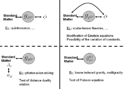
Figure 1: Summary of the proposed different classes of models. As discussed in the text, various tests can be designed to distinguish between them. The classes differ according to the kind of new fields and to the way they couple to the metric $g_{\mu\nu}$ and to the standard matter fields. Left column accounts for models where gravitation is described by general relativity while right column models describe a modification of gravity. In the upper line classes, the new fields dominate the matter content of the universe at low redshift. Upper-left models (class A) consist of models in which a new kind of gravitating matter is introduced. In the upper-right models (class C), a light field induces a long-range force so that gravity is not described by a massless spin-2 graviton only. This is the case of scalar-tensor theories of gravity. In this class, Einstein equations are modified and there may be a variation of the fundamental constants. The lower-right models (class D) corresponds to models in which there may exist massive gravitons, such as in some class of braneworld scenarios. These models predict a modification of the Poisson equation on large scales. In the last models (lower-left, class B), the distance duality relation may be violated.

This being defined, we can distinguish four general classes [13]. First are models in which gravity is not modified

1. Class A consists of models in which the acceleration is driven by the gravitational effect of new fields which are minimally coupled to gravity. It follows that they are not coupled to the standard matter fields or to dark matter and that one is adding a new sector

   $$S_{\rm de}[{\rm de};g_{\mu\nu}]$$

   to the action (1). To explain the acceleration of the universe, the new matter must have an equation of state, $w=P/\rho$ smaller than $-1/3$. As standard examples of this class of models, we can cite the standard $\Lambda$CDM model (which has the property to involve only 1 new parameter and no new field), quintessence models [20] which invoke a canonical scalar field slow-rolling today, solid dark matter models [21] induced by frustrated topological defects networks, tachyon models [22], Chaplygin gaz models [23] which try to unify dark matter and dark energy, and K-essence models [24] models invoking scalar fields with a non-canonical kinetic term.

2. Class B introduces new fields which do not dominate the matter content so that they do not change the expansion rate of the universe. These fields are coupled to photons and thus affect the observed dynamics of the universe but not the dynamics itself. In particular they are not required to have an equation of state smaller than $-1/3$. An example is provided by photon-axion oscillations in an external magnetic field [25] which aims at explaining the dimming of supernovae, not by an acceleration expansion but by the fact that part of the photons has oscillated into invisible axions. In that particular case, the electromagnetic sector is modified according to

   $$S_{\rm em}[A_{\mu};g_{\mu\nu}]\rightarrow S_{\rm em}[A_{\mu},a_{\mu};g_{\mu\nu}].$$

   A specific signature of these models would be a violation of the distance duality relation [13, 26], a possible violation of the variation of CMB temperature with redshift [$T_{\gamma}\propto(1+z)$] which seems to hold observationnally [27] and in the future, the determination of the luminosity from gravitational waves will be insensitive to such a coupling.

Then come models with a modification of gravity. Once such a possibility is considered, many new models arise [28]. Indeed in considering these modifications, one needs to take great care about the fact that the new theory is well defined [29] and stable both outside and inside matter (as an example theories such as $f(R_{\mu\nu})$ or $f(R_{\mu\nu\rho\sigma})$ involve extra massive spin-2 ghosts [30]; we also stress the Ostrogradksi theorem [31] as recently exposed in Ref. [29]). We can distinguish two classes,

1. Class C includes models in which a finite number of new fields are introduced. These fields couple to the standard model fields and some of them dominate the matter content (at least at late time). This is the case in particular of scalar-tensor theories in which a scalar field couples universally and leads to the class of extended quintessence models [32], chameleon models [33] or $f(R)$ models depending on the choice of the coupling function and potential. For these models, one would have a new sector

   $$S_{\varphi}[\varphi;g_{\mu\nu}]$$

   and the couplings of the matter fields will be modified according to

   $$S_{m}[{\rm mat};g_{\mu\nu}]\rightarrow S_{m}[{\rm mat}_{i};A^{2}_{i}(\varphi)g_{\mu\nu}].$$

   In the case where the coupling is not universal, a signature may be the variation of fundamental constants [34] and a violation of the universality of free fall. This was argued to be a general signature of quintessence models [35]. This is the case in particular in the runaway dilaton model [36]. This class also offers the possibility to enjoy $w<-1$ [37, 38] with a well-defined field theory and includes models in which a scalar field couples differently to standard matter field and dark matter [39].

2. Class D includes more drastic modifications of gravity with e.g. the possibility to have more types of gravitons (massive or not and most probably an infinite number of them). This is for instance the case of models involving extra-dimensions such as e.g. multi-brane models [40], multigravity [41], brane induced gravity [42] or simulated gravity [43]. In these cases, the new fields modified the gravitational interaction on large scale but do not necessarily dominate the matter content of the universe. Some of these models may also offer the possibility to mimick an equation of state $w<-1$.

These various modifications can indeed be combined to get more exotic models. Since models of classes C and D involve departure from general relativity, they have to pass the local tests on the deviation from general relativity (see Refs. [37, 44] for examples) both in weak field in the Solar system and in strong field (timing of pulsars). Both classes lead to a modification of the Poisson equation on sub-Hubble scales that can be tested using weak lensing or the large scale structure [45].

Let us stress two important points. First, these models do not address the cosmological constant problem (see Refs. [7, 10] for reviews on this aspect). Second, at the moment the analysis of the various cosmological data do not push for any time dependent equation of state and are completely compatible with the standard $\Lambda$CDM model (see e.g. Ref. [7] for a general review on the constraints, Refs. [1, 4, 5] for the constraints on a constant equation of state and Ref. [46] for the case of quintessence models) and there is no need at present for anything else but a cosmological constant [47].

In order to have some handle on the physics behind dark energy, one needs to detail the various signatures of these models. They may be of different natures: (1) dynamics of the background (related to the equivalent equation of state for each model), (2) properties of the growth of structure on sub-Hubble scales, (3) properties of perturbations involving super-Hubble scales, such as the CMB, (4) non-linear clustering, (5) local tests and (6) strong field effects such as gravitational waves production and low acceleration regimes (e.g. galaxy rotation curves).

From an observational point of view, we can briefly summarize the data sets that allow to probe these various regimes. (1) The background dynamics can be probed from the Hubble diagram [and more particularly using SN Ia; the angular distance-redshift relation from strong lensing; comoving volume; number counts vs. redshift using galaxy number counts; baryon acoustic oscillation (BAO); the CMB shift parameter; big-bang nucleosynthesis; and in the future the determination of luminosity distance from gravitational waves]. (2) The growth of structures in the Newtonian regime can be obtained from 3D-galaxy surveys (luminous matter), halo number count vs. redshift using clusters of galaxies (X-ray, optical/NIR counts and velocity dispersion, Sunyaev-Zel’dovich effect, strong and weak lensing) and galaxy redshift distribution (dark halos), Lyman-$\alpha$ forest, weak lensing (2D- survey but with the possible future development of tomography) that gives access to the matter and gravitational potential power spectra at different redshifts and on different scales. It is important to separate the linear and non-linear regimes that involves the regime (4). (3) Super-Hubble perturbations affect mainly the CMB in general and the integrated Sachs-Wolfe which, in particular when correlated with large scale structures, contains some information on dark energy. (5) Local tests are usually performed using the parameterized post-Newtonian formalism in the Solar system and (6) concerns mainly the timing of pulsars and the emission of gravitational waves.

From a theoretical point of view, it is important to determine which models are in fact two versions of the same model which means to determine the nature and couplings of the degrees of freedom (e.g. the fact that $f(R)$ models are nothing else but scalar-tensor theories [49] or that theories involving $f(R,\Box R,\ldots,\Box^{n}R)$ are $(n+1)$ scalar-tensor theories [50]; the relation between k-essence and quintessence [51]) and to which extent the same set of data can be reproduced by various theories. In this sense the determination of the number and nature of the new degrees of freedom are important and gives a theoretical estimate of the complexity of the theory much more accurate than the number of free parameters of a model. Obviously, a subset of all available data can be explained by models in different classes (see below) so that our classification will also help quantify the habiliy of a given set of data to distinguish between theoretical models, which is different from determining which family fits best.

From a more phenomenological point of view, it is often usefull to rely on an effective parameterization of the equation of state to describe the change in the dynamics of the expansion. Although it is a key empirical information on the rough nature of dark energy, a detailed description of its properties demands more thoughtful data interpretation. To be useful, the parameterization has to be realistic, in the sense that it should reproduce predictions of a large class of models, it has to minimize the number of free parameters, and it has to be related to the underlying physics (see e.g. Ref. [52]). Because the result of a data analysis will necessarily have some amount of parameterization dependence [53], choosing a specified physical model strategy seems preferable to break degeneracies. In particular, it enables to compute without any ambiguity their signature both in low and high redshift surveys, such as the cosmic microwave background. The increasingly flourishing number of models hampers to provide a comprehensive set of unambiguous predictions to constrain physical models one by one with present-day observations, but there are still several benefits in exploring dark energy this way, in particular when weak lensing surveys are used together with CMB observations. In this respect also, our classification may turn to be usefull.

It follows that one is stuck between pragmatism of the data analysis favouring parameterization of the equation of state (bottom-up approach) and the theorist point of view (top-down approach). It is indeed clear that the physical nature of dark energy will not directly come out of the observations and we need obviously to go beyond the measurement of $w$ to have any idea of the models or classes of models that are likely to be good candidate both to explain the observed universe and from a theoretical perspective. In this respect, constructing target models in each classes is a key issue. Both approaches are indeed complementary.

Here, we want to illustrate how perturbations are of importance when one wants to tackle down the physics behind the acceleration of the universe. In Section II, we start by recalling the properties of the background evolution and then we revisit the description of the perturbations and in particular we focus on their properties that can shed some light on the class of theoretical models that are best suited (see Fig. 1). This will lead us to propose a chain of tests to investigate dark energy. In Section III, we consider a first model inspired by brane world cosmology and then turn, in Section IV, to the more involved case of scalar-tensor theories of gravity.

II Distinguishing models

In this section, we compare the information that can be extracted from the background dynamics and the dynamics of density perturbation at small redshift. This will lead us to propose a chain of tests to characterize the properties of the dark energy.

II.1 Background evolution

Assuming the validity of the Copernician principle, the equation of state of the dark energy is obtained from the expansion history, assuming the standard Friedmann equation. It is thus given by the general expression (see e.g. Refs. [37, 54, 55])

$$3\Omega_{\rm de}w=-1+\Omega_{K}+2q,$$ (2)

$q$ being the deceleration parameter,

$$q=-\frac{a\ddot{a}}{\dot{a}^{2}}=-1+\frac{1}{2}(1+z)\frac{{\rm d}\ln H^{2}}{{\rm d}z}.$$ (3)

This expression does not assume the validity of general relativity or any theory of gravity but gives the relation between the dynamics of the expansion and the property of the matter that would lead to this acceleration if general relativity described gravity. Thus, it reduces to the ratio of the pressure to energy density only under this assumption. All the background information about dark energy is encapsulated in the single function $w$.

As long as the background dynamics is concerned, all the observations are related to the function $E(z)$ defined by

$$E(z) \equiv \frac{H(z)}{H_{0}}.$$ (4)

In particular, the angular distance is given by

$$D_{A}(z)=D_{H_{0}}\frac{S_{K}(\chi)}{1+z}$$ (5)

where $D_{H_{0}}=c/H_{0}$. The radial distance $\chi$ is defined by

$$\chi(z)=\frac{1}{a_{0}H_{0}}\int_{0}^{z}\frac{{\rm d}z^{\prime}}{E(z^{\prime})}$$ (6)

and the angular diameter distance $S_{K}$ is given by

$$S_{K}(\chi)=\left\{\begin{array}[]{lc}\sin(\sqrt{K}\chi)/\sqrt{K}&K>0\\ \chi&K=0\\ \sinh(\sqrt{-K}\chi)/\sqrt{-K}&K<0\\ \end{array}\right..$$ (7)

In the case where the distance duality relation holds, the luminosity distance is given by

$$D_{L}(z)=(1+z)^{2}D_{A}(z),$$ (8)

but this may not be the case in models of the class B.

II.2 Parameterization of the equation of state

Most data, and in particular supernovae data, are being analyzed using a general parameterization of the equation of state. These parameterizations are useful to extract model-independent information from the observations but the interpretation of these parameters and their relation with the physical models are not always straightforward.

As a first example, recall that general parameterizations of the equation of state as

$$w(a)=w(a_{0})+[w(a_{m})-w(a_{0})]\ \Gamma(a,a_{t},\Delta)$$ (9)

were shown to allow an adequate treatment of a large class of quintessence models [56, 57]. It involves four parameters $\{w(a_{0}),w(a_{m}),a_{t},\Delta\}$ and a free function $\Gamma$ varying smoothly between one at high redshift to zero today. Even though it reproduces the equation of state of most quintessence models, it is not economical in terms of number of parameters since most quintessence potentials involve one or two free parameters. If one assumes that the parameterization is supposed to describe the dynamics of a minimally coupled scalar field, the knowledge of $w$ is indeed sufficient but in a more general case one would need more information. The background dynamics depends on the potential and its first derivative, which can be related to $w$ and its derivative. Accounting for perturbations, one needs to know the second derivative of the potential which can be inferred from $\ddot{w}$ [58].

Since we expect dark energy to have observable consequences on the dynamics only at late time, one can consider an equation of state obtained as a Taylor expansion around a pivot point,

$$\widetilde{w}=w_{*}+w_{a}\left(\frac{1}{1+z_{*}}-\frac{1}{1+z}\right).$$ (10)

This form depends on only three parameters and is a generalization of the parameterization proposed by [59] and then [60] where $z_{*}=0$. Whatever the expression for $w$, it is easy to sort out that

$$\rho_{\rm de}^{\prime}=-3(1+\widetilde{w})\rho_{\rm de}$$ (11)

where a prime denotes a derivative with respect to the number of $e$-folds, $p=\ln(a/a_{0})$. It follows that

$$\rho_{\rm de}=\rho_{{\rm de}0}\,\exp\left[{-3\int_{0}^{p}(1+\widetilde{w}){\rm d}p}\right]$$ (12)

and thus

$$\frac{H^{2}}{H_{0}^{2}}=\Omega_{{\rm m}0}\hbox{e}^{-3p}+\Omega_{K0}\hbox{e}^{-2p}+\Omega_{{\rm de}0}\hbox{e}^{-3\int_{0}^{p}(1+\widetilde{w}){\rm d}p}.$$ (13)

Two considerations are in order when using such a parameterization. First, the redshift band on which this is a good approximation of the equation of state is a priori unknown. Clearly, compared with the form (9), it is unlikely to describe dark energy up to recombination time. Secondly, when combining observables at different redshift such as weak lensing, Sn Ia and CMB, one should choose the value of $z_{*}$ in such a way that the errors in $w_{*}$ and $w_{a}$ are uncorrelated [61] and the pivot redshift is the redshift at which $w$ is best constrained. In particular, it was argued that it is important to choose $z_{*}$ for distance-based measurements. The problem lies in the fact that the pivot redshift is specific to the observable. In this respect, dark energy models defined by a Lagrangian are more suitable, yielding to a definite equation of state as a function of redshift, hence more general than a Taylor expansion around a pivot point. Eventually, one can read out the values of $w_{*}$ and $w_{a}$ at whatever redshift. This complication, arising when one wants to combine datasets with different $z_{*}$, will also make it more difficult to infer constraints on the physical models from the constraints on the parameterization (see Refs. [46, 62] for examples).

There is an alternative way to get a first hint on the nature of dark energy. It may be useful to consider the plane $(w,w^{\prime})$ where $w^{\prime}\equiv{\rm d}w/{\rm d}p$. It was recently shown [63, 64] that quintessence models occupy a narrow part of this plane (assuming $z_{*}=0$). As discussed later on, the way to relate these parameters to a physical model (that is the reciproque) is difficult.

In conclusion, a class of equations of states or the $(w,w^{\prime})$ analysis are usefull tools to constraint a class of theoretical models independently of the details of each model and the parameterization must be designed for this class of models. In such a case the position in the $(w,w^{\prime})$ can also be related to a particular model in this class. For instance, in the case of quintessence models where the acceleration is due to the gravitational effect of a slow-rolling minimally coupled scalar field, the position in the $(w,w^{\prime})$ plane can be related to the slow-roll parameters

$$\varepsilon=\frac{1}{16\pi G}\left(\frac{V^{\prime}}{V}\right)^{2},\qquad\eta=\frac{1}{8\pi G}\left(\frac{V^{\prime\prime}}{V}\right),$$ (14)

characterizing the shape of the potential $V$ close to the value of the scalar field today since $w\simeq-1+2\varepsilon/3$ and $w^{\prime}\simeq-4\varepsilon(\eta-2\varepsilon)/3$. Unfortunately, this cannot determine the model since the same position can be reached by various models from different classes.

For background evolution, we thus have various parameterizations that describe class A models and include the $\Lambda$CDM as a subcase. They enable to quantify, within this particular class, how close from a $\Lambda$CDM the background dynamics allows to be. In the particular case of quintessence, the relation with the physical parameters is clear but one should impose a prior on the parameterizations to ensure that $w\geq-1$ as is the case for these models (see e.g. Ref. [46] for a comparison of a data analysis based on a model and a parameterization). Indeed, great care is required when interpreting constraints obtained from such a parameterization when relaxing this prior.

II.3 Taking perturbations into account

From the study of the background dynamics, one can, in principle, determine or constrain $w(a)$. Other sets of data, such as weak lensing and large scale structures, involve density perturbations. Assuming that the metric of spacetime takes the form

$${\rm d}s^{2}=-(1+2\Phi){\rm d}t^{2}+(1-2\Psi)a^{2}\gamma_{ij}{\rm d}x^{i}{\rm d}x^{j},$$ (15)

where $\gamma_{ij}$ is the metric of the spatial section, the evolution of density perturbations on sub-Hubble scales is dictated by

$$\ddot{\delta}_{\rm m}+2H\dot{\delta}_{\rm m}-\frac{1}{a^{2}}\Delta\Phi=\mathcal{S}_{\rm de}.$$ (16)

This equation derives from the Euler and conservation equations on sub-Hubble scales, that is from the conservation of the stress-energy tensor of matter. It could inherit a source term $\mathcal{S}_{\rm de}\not=0$ if the presureless matter is coupled to other matter species (e.g. in class C).

To close this equation, one needs to use Einstein equations to express $\Phi$. Assuming general relativity and a $\Lambda$CDM model, the Poisson equation takes its standard form

$$\Delta\Psi=4\pi G\rho_{\rm m}a^{2}\delta_{\rm m}=\frac{3}{2}\Omega_{\rm m}H^{2}a^{2}\delta_{\rm m},$$ (17)

and the two gravitational potentials are related by

$$\Phi-\Psi=0$$ (18)

since the anisotropic stress of radiation is negligible in that regime. When considering dark energy models, one has to allow possible modifications of these two equations.

First, the second Einstein equation can enjoy a non-vanishing anisotropic stress due to the dark energy sector so that it takes the general form

$$\Delta(\Phi-\Psi)=\Pi_{\rm de}$$ (19)

where $\Pi_{\rm de}$ can be decomposed as $\Pi_{\rm de}=8\pi GP_{\rm de}a^{2}\Delta\pi_{\rm de}$. This term leads to a general source term $\mathcal{S}_{\rm de}+\Pi_{\rm de}/a^{2}$ in Eq. (16) but it is worthwile making the distinction because $\Pi_{\rm de}$ alone will be involved in lensing observations that depend on $\Phi+\Psi$. All classes can induce such a term.

Second, the density perturbation of the dark energy may be non negligible in the Poisson equation and, as in the case with a modification of gravity, one can expect a modification of proportionality coefficient that may even be scale dependent. So we will assume that the general form of the Poisson equation is, in Fourier space,

$$-k^{2}\Phi=4\pi Ga^{2}F_{\rm m}(k,H)\rho_{\rm m}\delta_{\rm m}+\Delta_{\rm de}.$$ (20)

If $F_{m}$ depends on $k$ then the modification will not be degenerate with the normalisation of the amplitude of the matter power spectrum and can be tested [65] otherwise one will have to use the growth history to determine whether $F_{\rm m}=1$ or not. Such a term can arise in classes C (see e.g. Ref. [66]) and D (see Ref. [67]). We emphasize that for classes A and B, the growth factor is scale independent and that the primordial scale-dependence and the growth factor decouple. This may not be the case in classes C and D when $F_{\rm m}$ is scale dependent. Thus, it is safer to distinguish $P_{\rm m}(k,z)$ and $P_{\Phi}(k,z)$.

It follows that in general, the equation of evolution of the growth factor is expected to take the form

$$\ddot{D}+2H\dot{D}-4\pi G\rho F_{\rm m}D=\frac{\Delta_{\rm de}}{a^{2}}+\mathcal{S}_{\rm de}.$$ (21)

Indeed, such an equation is not closed and one needs either to propose a parametrization of the source term or explicit the evolution equations of the dark sector. Note that while the growth factor depends on ($F_{\rm m}$, $\Delta_{\rm de}$, $\mathcal{S}_{\rm de}$), weak lensing involves the combination $\Delta(\Phi+\Psi)=8\pi G\rho a^{2}F_{\rm m}\delta_{\rm m}+2\Delta_{\rm de}-\Pi_{\rm de}$ [68] so that combining them may be very fruitful.

In conclusion, the evolution of perturbations at low redshift of the various classes of models can be characterized in the Newtonian regime by $(\mathcal{S}_{\rm de},\Delta_{\rm de},F_{\rm m},\Pi_{\rm de})$. Models of the class A satisfy $(\mathcal{S}_{\rm de},\Delta_{\rm de},F_{\rm m},\Pi_{\rm de})=(0,\Delta_{\rm de},1,\Pi_{\rm de})$; for instance, a $\Lambda$CDM model has

$$(\mathcal{S}_{\rm de},\delta_{\rm de},F_{\rm m},\Pi_{\rm de})=(0,0,1,0)$$ (22)

while for quintessence models, $\delta\rho_{\rm de}=\dot{\varphi}\delta\dot{\varphi}-\dot{\varphi}^{2}\Phi+V^{\prime}\delta\varphi$ so that

$$(\mathcal{S}_{\rm de},\Delta_{\rm de},F_{\rm m},\Pi_{\rm de}) \simeq \left(0,0,1,0\right)$$ (23)

where $\varphi$ is the quintessence field and $\delta\varphi$ its perturbation. This shows in particular that quintessence and $\Lambda$CDM can only be distinguished, at low redshift, on the basis of their equation of state. Models of the class B have the same characteristics than a $\Lambda$CDM for the density perturbation evolution but have an effective equation of state that may differ from $w=-1$. Models of the classes C and D have more general $(\mathcal{S}_{\rm de},\Delta_{\rm de},F_{\rm m},\Pi_{\rm de})$ and in particular $F_{\rm m}\not=1$. We shall give two examples further on.

II.4 Summary

Figure 2: A possible chain of tests to unveil the nature of dark energy. The goal is to start from the more general hypothesis and to incorporate new data and information one by one in order to check at each step if the hypothesis underlying the equations used in the analysis hold or not. Here $\bar{D}_{+}$ refers to the growth factor predicted from $w(z)$ assuming general relativity. In particular, it may turn out that a deviation from the Poisson equation may be detected while no deviation from $w=-1$ is established. This would however require to extend the minimal $\Lambda$CDM.

We have argued that the different models appearing in the classification presented in Fig. 1 can be characterized by a set of functions including the equation of state to describe the background dynamics and $(\mathcal{S}_{\rm de},\delta_{\rm de},F_{\rm m},\Pi_{\rm de})$ for the evolution of the perturbations at low redshift. In most cases, the dependence on the primordial spectrum and on the dark energy sector decouple in the Newtonian regime. Indeed, more information would be needed to treat CMB anisotropies and strong field phenomena.

This description can help to get some handle the nature of dark energy and in particular can give a way to organize the theoretical landscape and the way to distinguish between classes. In particular, it will be usefull to define both a target model and parameterizations in each class so that the distance to the $\Lambda$CDM in each category can be quantified. Such parameterizations exist for the class A but they need to be generalized to other classes and the constraints on the parameters of these parameterizations for them to describe physical models actually in these classes should be established.

Let us also mention a difference with a simple fit of models to data. In this case, one ususaly minimizes the information of the data and the theory together, $I(D,T)$ taking into account a penalty, $I(T)$, that depends on the number of the free parameters of the theory [69]. The total information reduces to $I(D,T)=I(D|T)+I(T)$ with $I(D|T)$ being the opposite of the likelyhood and various prescriptions for $I(T)$, all depending on the number of free parameters, exist but in fact it depends on the complexity of the theory. It is in general difficult to define but it is related to the number, nature and couplings of the new fields of the theory. To this respect, the $\Lambda$CDM model is the simplest since it involves only 1 new parameter and no new field. Relying on null test (or exclusion tests) is a way to indicate the degree of complexity required without having to consider such a statistical issue in the first place (see Ref. [70] for the implication concerning dark energy).

It follows from the previous discussion that various questions arise in order to grasp some of the physics behind dark energy. We propose the chart in Fig. 2 to address them and outline the dark energy sector. It is based on a series of consistency checks trying to exclude the most simple models in order to determine how complex a minimal model should be. It also tries to determine to which extent data can discriminate between the various classes and calls for the construction of new tests. At the heart of it, is the question of the necessity to extend the standard $\Lambda$CDM and to determine, in a robust way, how close from it we must be. Indeed demonstrating the time variabiliy of $w$ is difficult to proove but it may be that other signatures will be easier to obtain [71].

III First example: DGP cosmology

The Dvali-Gabadadze-Porrati (DGP) brane-world model [42, 72] is constructed from a brane embedded in a 5-dimensional Minkowski bulk. It was shown that because of gravity leakage to the bulk, it leads to a modification of gravity on large scales and could explain the recent acceleration phase. The characteristic scale, $r_{c}$, at which the modification of gravity manifests itself is related to the two mass scales of the model, the usual 4-dimensional Planck mass and the 5-dimensional Planck mass, $M_{5}$. When $M_{5}\sim 10-100$ MeV, $r_{c}$ is typically of the order of $c/H_{0}$. Interestingly, this model involves only 1 extra-parameter, as the standard $\Lambda$CDM, but involves new fields.

III.1 Summary of the cosmological properties

In the DGP model (see Refs. [42, 72] for a description of the model), the Friedmann equation takes the form

$$H^{2}+\frac{K}{a^{2}}=\left(\sqrt{\frac{8\pi G}{3}\rho+\frac{1}{4r_{c}^{2}}}+\frac{\varepsilon}{2r_{c}}\right)^{2}$$ (24)

and we consider the $\varepsilon=1$ case. $r_{c}$ is the new parameter of the model. We focuse to the low redshift universe where $\rho$ is dominated by presureless matter. We define

$$\Omega_{\rm c0}=\frac{1}{4r_{c}^{2}H_{0}^{2}},$$ (25)

so that it rewrites as

$$E^{2}(z)\equiv\frac{H^{2}}{H_{0}^{2}}=\Theta^{2}+\Omega_{K0}(1+z)^{2}$$ (26)

where we have defined

$$\Theta(z)\equiv\sqrt{\Omega_{\rm c0}}+\sqrt{\Omega_{\rm c0}+\Omega_{{\rm m}0}(1+z)^{3}}.$$ (27)

It follows that we have the constraint

$$\Theta^{2}(0)+\Omega_{K0}=\left(\sqrt{\Omega_{\rm c0}}+\sqrt{\Omega_{\rm c0}+\Omega_{{\rm m}0}}\right)^{2}+\Omega_{K0}=1$$ (28)

the solution of which is

$$\Omega_{\rm c0}=\frac{(-1+\Omega_{{\rm m}0}+\Omega_{K0})^{2}}{4(1-\Omega_{K0})}.$$ (29)

By comparing Eq. (26) with its standard form, we deduce that

$$\frac{8\pi G\rho_{\rm de}}{3H_{0}^{2}}=2\sqrt{\Omega_{\rm c0}}\,\Theta(z),$$ (30)

or equivalently

$$\Omega_{\rm de}=2\sqrt{\Omega_{\rm c}}\left[\sqrt{\Omega_{\rm c}}+\sqrt{\Omega_{\rm c}+\Omega_{\rm m}}\right],$$ (31)

where

$$\Omega_{\rm c}=\Omega_{\rm c0}\frac{H_{0}^{2}}{H^{2}},\quad\Omega_{\rm m}=\Omega_{{\rm m}0}(1+z)^{3}\frac{H_{0}^{2}}{H^{2}}.$$

In particular, $\Omega_{\rm de}+\Omega_{\rm m}+\Omega_{K}=1$ is equivalent to the constraint (28) when evaluated today. Using the expression (26) we obtain that

$$1+w(z)=\frac{\Omega_{{\rm m}0}(1+z)^{3}}{2\Theta(z)\sqrt{\Omega_{\rm c0}+\Omega_{{\rm m}0}(1+z)^{3}}}$$ (32)

whatever the curvature. It is easy to sort out that

$$w^{\prime}=\frac{{\rm d}w}{{\rm d}p}=-\frac{3}{4}\frac{\sqrt{\Omega_{\rm c0}}\Omega_{{\rm m}0}(1+z)^{3}}{[\Omega_{\rm c0}+\Omega_{{\rm m}0}(1+z)^{3}]^{3/2}}.$$ (33)

As a first consequence of this analysis, Fig. 3 shows that today the background evolution of DGP models can be mimicked by quintessence models. Note that the zone of the plane $(w_{0},{\rm d}w_{0}/{\rm d}p)$ that corresponds to DGP models remains very thin even when we allow $\Omega_{K0}$ to vary between $-1$ and $1$ and $\Omega_{{\rm m}0}$ between 0 and 1.

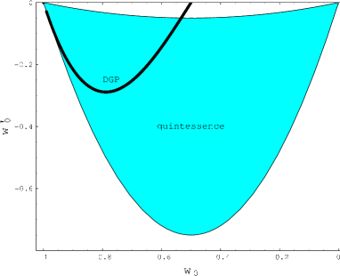
Figure 3: In the plane $(w,w^{\prime})$, the filled zone corresponds to quintessence models while the very thin black zone corresponds to DGP models. We have allowed $\Omega_{K0}$ to vary between $-1$ and $1$ and $\Omega_{{\rm m}0}$ between 0 and 1.

III.2 Models with equivalent background evolution

III.2.1 Fitting the equation of state with a parameterization

The matching to a given equation of state can be performed in various ways. First, once $z_{*}$ has been chosen, we can require to fit $(w,w^{\prime})$ at the pivot redshift, so that

$$w_{*}=w(z_{*}),\qquad w_{a}=-(1+z_{*})w^{\prime}(z_{*}).$$ (34)

Another route is to require that the equation of state has its correct value today and at a redshift $z_{p}$ so that

$$w_{*}=w(z_{*}),\qquad w_{a}=[w(z_{p})-w(z_{*})]\frac{(1+z_{p})(1+z_{*})}{z_{p}-z_{*}}.$$ (35)

In Fig. 4, we compare these two fits of the DGP equation of state (32) assuming $z_{*}=0$ and choosing $z_{p}=3$ and $z_{p}=100$. By construction both matching lead to the correct value of the equation of state today ($w_{*}=w_{0}$) but the derivative differs by $6.6\,\%$ and $-5.3\,\%$. Indeed these are very small deviations but they may be important while trying to infer whether a constraint on $(w_{0},w^{\prime}_{0})$ points toward a DGP model or a quintessence model. So the question that arises is how a measured $(w_{*},w_{a})$ is actually related to the constraint plane depicted in Fig. 3, and to the physical parameters of the model.

Interestingly, as shown in Fig. 5, the error induced on the growth factor coming from the error in the fitting of the equation of state is smaller than 1%. This implies that one cannot distinguish between the three parametrizations studied in Fig. 4 from the study of perturbations.

Figure 4: Comparison of the fits of the DGP equation. The solid line corresponds to the fit defined in Eq. (34) while the dashed and dotted lines correspond to the fit defined in Eq. (35) respectively with $z_{p}=3$ and $z_{p}=1000$. We have assume $\Omega_{{\rm m}0}=0.3$ and $\Omega_{K0}=0$.

Figure 5: Comparaison of linear growth factor for the same fits as in Fig. 6 to the equivalent quintessence model.

III.2.2 Equivalent scalar field model

We can even go a bit further and construct explicitely the quintessence model that reproduces the DGP dynamics for the background.

Quintessence models reduce to the dynamics of a minimally coupled scalar field, $Q$, evolving in a potential $V(Q)$. The model is completely specified once the potential is given. It is thus clear that the energy density is given by

$$\rho_{Q}=\frac{1}{2}\dot{Q}^{2}+V$$ (36)

and the equation of state is

$$w_{Q}=\frac{\dot{Q}^{2}-2V}{\dot{Q}^{2}+2V}.$$ (37)

Inverting these two relations, one can reconstruct the potential [73] mimicking a dark energy component characterized by $\{\rho_{\rm de}(a),w_{\rm de}(a)\}$ since we have

$$\dot{Q}^{2} = \rho_{\rm de}(a)[1+w_{\rm de}(a)],$$

$$V = \frac{1}{2}\rho_{\rm de}(a)[1-w_{\rm de}(a)].$$ (38)

It follows that the parametric expression of the potential is

$$V(z) = \frac{1}{2}\rho_{\rm de}(z)[1-w_{\rm de}(z)],$$ (39)

$$\frac{{\rm d}Q}{{\rm d}z} = \pm\frac{\sqrt{\rho_{\rm de}(z)[1+w_{\rm de}(z)]}}{(1+z)H(z)}.$$ (40)

We can arbitrarily choose the sign of ${\rm d}Q/{\rm d}z$. Using Eq. (30) and defining $\mathcal{V}=8\pi GV/3H_{0}^{2}$ and $\mathcal{Q}=\sqrt{8\pi G/3}Q$, this system take the form

$$\mathcal{V}(z) = \sqrt{\Omega_{\rm c0}}[1-w_{\rm de}(z)]\Theta(z),$$ (41)

$$\frac{{\rm d}\mathcal{Q}}{{\rm d}z} = \frac{\left\{2\sqrt{\Omega_{\rm c0}}[1+w_{\rm de}(z)]\Theta(z)\right\}^{1/2}}{(1+z)E(z)}.$$ (42)

Once $(\Omega_{{\rm m}0},\Omega_{K0})$ is fixed, $\Omega_{\rm c0}$ is determined and the DGP model we want to mimick is completely specified. It follows that $w_{\rm de}$ is given by Eq. (32) and $E(z)$ by Eq. (26) and we have a unique potential obtained from the integration of the system (41-42).

Figure 6 depicts the potentials of the quintessence models that give the same background dynamics that DGP model for $\Omega_{{\rm m}0}=0.3$ and $\Omega_{K0}=0,\pm 0.3$. Indeed, to choose one or the other model (DGP or quintessence) has some importance and takes some theoretical prejudices into account.

Note also that, as long as we assume that the growth of density perturbations, is not modified and is given by a form (23), the two models cannot be distinguished.

Figure 6: Reconstruction of the potential of a quintessence model that gives the same background evolution than the DGP model when $\Omega_{{\rm m}0}=0.3$ and $\Omega_{K0}=0$ (solid), $\Omega_{K0}=0.3$ (dashed) and $\Omega_{K0}=-0.3$ (dotted).

III.3 Growth of density perturbation

The previous result assumed that the growth of density perturbations is dictated by the standard equation. For the DGP model, this is not the case and two routes have been followed. In the first, five dimensional effects were neglected [74], which we will refer to as DGP-4D, so that

$$(\mathcal{S}_{\rm de},\Delta_{\rm de},F_{\rm m},\Pi_{\rm de})=\left(0,0,\frac{2Hr_{c}}{2Hr_{c}-1},0\right).$$

Unfortunately this setting is not compatible with the Bianchi identity. It was recently argued [67] that when five dimensional effects are taken into account we should have

$$(\mathcal{S}_{\rm de},\Delta_{\rm de},F_{\rm m},\Pi_{\rm de})=\left(0,0,1+\frac{1}{3\beta},\frac{8\pi G}{3\beta}\rho_{\rm m}a^{2}\delta_{\rm m}\right),$$

with

$$\beta = 1-2r_{c}H\left(1+\frac{\dot{H}}{3H^{2}}\right)$$ (43)

$$= 1-\frac{E}{\sqrt{\Omega_{\rm c0}}}\left[1+\frac{1}{3}(\ln E)^{\prime}\right].$$

We shall refer to this case as DGP-5D. The influence of this modification of the growth factor on lensing observables was recently studied in Ref. [75].

From these definitions, we deduce that in the DGP-4D case, the equation of evolution of the growth factor (21) can be rewritten in terms of the growth variable, $g\equiv D/a$, as

$$g^{\prime\prime} + \left[4+\left(\ln E\right)^{\prime}\right]g^{\prime}$$ (44)

$$+ \left[3+\left(\ln E\right)^{\prime}-\frac{3}{2}\Omega_{\rm m}\frac{E}{E-\sqrt{\Omega_{\rm c0}}}\right]g=0$$

where we have used that $2Hr_{c}=E/\sqrt{\Omega_{\rm c0}}$. In the DGP-5D case, it takes the form

$$g^{\prime\prime} + \left[4+\left(\ln E\right)^{\prime}\right]g^{\prime}$$ (45)

$$+ \left[3+\left(\ln E\right)^{\prime}-\frac{3}{2}\Omega_{\rm m}\left(1+\frac{1}{3\beta}\right)\right]g=0.$$

These two solutions have to be compared to the equivalent quintessence model with same background dynamics for which

$$(\mathcal{S}_{\rm de},\Delta_{\rm de},F_{\rm m},\Pi_{\rm de})\simeq\left(0,0,1,0\right).$$

Fig. 7 compares the linear growth factor for the DGP-4D, DGP-5D and equivalent quintessence model. First, we see that the equivalent quintessence model can be discriminated from the DGP model on the basis of the perturbations (almost 20% difference at redshift 0). This clearly illustrates the (trivial) fact that perturbations encode extra-information than the one given by the bakground dynamics.

We also see that the “theoretical” uncertainty on the way to deal with perturbation can lead to uncertainty of order 5-10% on the growth factor. It is important to try estimate this uncertainty, particularly for models that deviates significantly from the standard ones.

Figure 7: (Top) Comparison of the linear growth factors of the DGP-5D (solid), DGP-4D (dash) and equivalent quintessence (dot) models. (Bottom), the relative error with respect to the DGP-5D have been computed and can become large. We have assumed $\Omega_{{\rm m}0}=0.3$ and $\Omega_{K0}=0$.

III.4 Summary

We have considered a DGP model that belongs to the class D. Using the fact that the effective equation of state is explicitely known we have compared it to a standard parameterization. We have constructed a quintessence model (class A) sharing exactly the same background dynamics. After sorting out the form of $(\mathcal{S}_{\rm de},\Delta_{\rm de},F_{\rm m},\Pi_{\rm de})$, we have shown that knowledge of the density perturbation can, as expected, help distinguishing these models.

This gives an explicit example in which the background dynamics cannot discriminate between a class A and class D models. It also shows that one should also try to quantify the “uncertainty” of the theoretical models, a difficult task indeed.

IV Second example: Scalar-tensor theories

As a second example, we consider scalar-tensor theories of gravity, which is the simplest example of a model of class C.

IV.1 Overview

In scalar-tensor theories of gravity, gravity is mediated not only by a spin-2 graviton but also by a spin-0 scalar field that couples universally to matter fields (this ensures the universality of free fall). In the Jordan frame, the action of the theory takes the form

$$S = \int\frac{{\rm d}^{4}x}{16\pi G_{*}}\sqrt{-g}\left[F(\varphi)R-g^{\mu\nu}Z(\varphi)\varphi_{,\mu}\varphi_{,\nu}-2U(\varphi)\right]$$ (46)

$$\qquad+S_{m}[\psi;g_{\mu\nu}]$$

where $G_{*}$ is the bare gravitational constant from which we define $\kappa_{*}=8\pi G_{*}$. This action involves three arbitrary functions ($F$, $Z$ and $U$) but only two are physical since there is still the possibility to redefine the scalar field. $F$ needs to be positive to ensure that the graviton carries positive energy. $S_{m}$ is the action of the matter fields that are coupled minimally to the metric $g_{\mu\nu}$.

It follows that the Friedmann equations in Jordan frame take the form

$$3F\left(H^{2}+\frac{K}{a^{2}}\right) = 8\pi G_{*}\rho+\frac{1}{2}Z\dot{\varphi}^{2}-3H\dot{F}+U$$ (47)

$$-2F\left(\dot{H}-\frac{K}{a^{2}}\right) = 8\pi G_{*}(\rho+P)+Z\dot{\varphi}^{2}$$ (48)

$$\qquad+\ddot{F}-H\dot{F}.$$

The Klein-Gordon and conservation equations are given by

$$Z(\ddot{\varphi}+3H\dot{\varphi})=3F_{\varphi}\left(\dot{H}+2H^{2}+\frac{K}{a^{2}}\right)$$

$$\qquad\qquad-\frac{1}{2}Z_{\varphi}\dot{\varphi}^{2}-U_{\varphi}$$ (49)

$$\dot{\rho}+3H(\rho+P)=0,$$ (50)

where a subscript $\varphi$ stands for a derivative with respect to the scalar field.

These equations define an effective gravitational constant

$$G_{\rm eff}=G_{*}/F.$$ (51)

This constant, however, does not correspond to the gravitational constant effectively measured in a Cavendish experiment,

$$G_{\mathrm{cav}}=\frac{G_{*}}{F}\left(1+\frac{F_{\varphi}^{2}}{2ZF+3F_{\varphi}^{2}}\right),$$ (52)

an expression valid when the scalar field is massless. Solar system constraints on the post-Newtonian parameters imply that $F_{\varphi 0}^{2}/F_{0}\lesssim 4\times 10^{-5}$ so that they do not differ significantly at low redshift.

IV.2 Sub-Hubble perturbations

The general cosmological perturbations have been studied in various articles [66, 77] and we concentrate to the sub-Hubble regime.

The conservation equation of the standard matter are similar to the ones in general relativity so that $\mathcal{S}_{\rm de}=0$. In the Newtonian regime, it can be shown that

$$\Psi-\Phi=\frac{F_{\varphi}}{F}\delta\varphi,$$ (53)

so that non-minimal coupling induces an extra-contribution to the anisotropic stress,

$$\Pi_{\rm de}=-\frac{F_{\varphi}}{F}\Delta\delta\varphi.$$ (54)

The Poisson equation takes the form

$$\Delta\Phi=4\pi\frac{G_{*}}{F}\rho a^{2}\delta_{m}+\Delta_{\rm de}.$$ (55)

Using the definition (52) of the gravitational constant, we deduce that

$$F_{\rm m}=\frac{F_{0}}{F}\left(1+\frac{F_{,\varphi}^{2}}{2F+3F_{\varphi}^{2}}\right)^{-1}_{0}\simeq\frac{F_{0}}{F}$$ (56)

where the last equality has been drawn using the Solar system constraints and should hold at low redshift (see e.g. Refs. [66, 77] for explicit examples of the redshift variation of this quantitiy). It can be shown [66] that on sub-Hubble scales, $\Delta_{\rm de}=-(F_{\varphi}/2F)\Delta\delta\varphi$ so that scalar-tensor models are characterized by

$$(\mathcal{S}_{\rm de},\Delta_{\rm de},F_{\rm m},\Pi_{\rm de}) \simeq \left(0,-\frac{F_{\varphi}}{2F}\Delta\delta\varphi,\frac{F_{0}}{F},-\frac{F_{\varphi}}{F}\Delta\delta\varphi\right).$$

To go further, one needs to determine $\delta\varphi$ and thus use the Klein-Gordon equation which reduces, in that limit, to

$$\left(\Delta-U_{\varphi\varphi}a^{2}\right)\delta\varphi=F_{\varphi}\Delta(\Phi-2\Psi)$$ (57)

from which we deduce

$$\left[U_{\varphi\varphi}a^{2}-\left(1+2\frac{F_{\varphi}^{2}}{F}\right)\Delta\right]\delta\varphi=F_{\varphi}\Delta\Phi.$$ (58)

It follows that $\Pi_{\rm de}$ and $\Delta_{\rm de}$ are directly proportional to $\Phi$ and the Poisson equation is given by

$$-k^{2}\Phi=4\pi\frac{G_{*}}{F}\left[1-\frac{k^{2}F_{\varphi}^{2}}{(2ZF+4F_{\varphi}^{2})k^{2}+2U_{\varphi\varphi}F}\right]^{-1}\rho_{\rm m}a^{2}\delta_{\rm m}.$$ (59)

When $U_{\varphi\varphi}$ is much smaller than the wavelength of the modes, which a good approximation in most models such as extended quintessence models, Eq. (58) reduces to

$$\Delta\Phi\simeq 4\pi G_{\mathrm{cav}}\rho a^{2}\delta_{m}$$ (60)

where $G_{\mathrm{cav}}$ is defined by Eq. (52).

This analysis shows that scalar-tensor models are characterized by

$$(\mathcal{S}_{\rm de},\Delta_{\rm de},F_{\rm m},\Pi_{\rm de}) \simeq \left(0,0,\frac{G_{\mathrm{cav}}}{{G_{\mathrm{cav}0}}},\frac{F^{2}_{\varphi}}{F+2F_{\varphi}^{2}}\Delta\Phi\right)$$ (61)

$$\simeq \left(0,0,\frac{G_{\mathrm{cav}}}{{G_{\mathrm{cav}0}}},0\right).$$

$F_{\rm m}$ is indeed time dependent but $k$ independent. Two functions of $z$ characterize scalar-tensor models, the equation of state and $F_{\rm m}$, they are related to the two free functions of the theory ($F$ and $U$) and influence both the background evolution and the linear growth of density perturbations.

IV.3 Class C vs class A

As a first exercice, we can quantify the effect of $F_{\rm m}$ and compare a scalar-tensor theory with a model of class A with the same background dynamics. For that purpose, we need to reconstuct the scalar-tensor theory, which can be achieved by using th background equations in the form [77]

$$\frac{{\rm d}^{2}F}{{\rm d}z^{2}}+\left[\frac{{\rm d}\ln E}{{\rm d}z}-\frac{4}{1+z}\right]\frac{{\rm d}F}{{\rm d}z}+\left[\frac{6}{(1+z)^{2}}-\frac{2}{1+z}\frac{{\rm d}\ln E}{{\rm d}z}-4\frac{\Omega_{K0}}{E^{2}}\right]F=\frac{2\bar{U}}{(1+z)^{2}E^{2}}+3\frac{1+z}{E^{2}}\Omega_{{\rm m}0}F_{0}$$ (62)

$$Z\left(\frac{{\rm d}\varphi}{{\rm d}z}\right)^{2}=-\frac{6}{1+z}\frac{{\rm d}F}{{\rm d}z}+\frac{6F}{(1+z)^{2}}-\frac{2\bar{U}}{(1+z)^{2}E^{2}}-6\frac{1+z}{E^{2}}\Omega_{{\rm m}0}F_{0}-6\frac{F}{E^{2}}\Omega_{K0}$$ (63)

where $\bar{U}=UH_{0}^{2}$ and $\Omega_{{\rm m}0}=8\pi G_{\mathrm{cav}0}\rho_{{\rm m}0}/3H_{0}^{2}\sim 8\pi G_{*}\rho_{{\rm m}0}/3F_{0}H_{0}^{2}$. As was initially shown in Ref. [77], the knowledge of $H(z)$ and $D(z)$ allow to reconstruct the two free functions that appear in the microscopic Lagrangian of the scalar-tensor theory.

The reconstruction can be performed in Jordan frame but it is usefull to shift to Einstein frame where mathematical consistency is easier to check. To do so, one perform the conformal transformation $g_{\mu\nu}^{*}=F(\varphi)g_{\mu\nu}$ so that the potential, $V$, coupling $A$, and spin-0 degree of freedom, $\varphi_{*}$, are related to the Jordan frame quantity by

$$A(\varphi_{*}) = F^{-1/2}(\varphi),$$ (64)

$$2V(\varphi_{*}) = F^{-2}(\varphi)U(\varphi),$$ (65)

$$\left(\frac{{\rm d}\varphi_{*}}{{\rm d}\varphi}\right)^{2} = \frac{3}{4}\left(\frac{{\rm d}\ln F(\varphi)}{{\rm d}\varphi}\right)^{2}+\frac{Z(\varphi)}{2F(\varphi)}.$$ (66)

We usually define $\alpha={\rm d}\ln A/{\rm d}\varphi_{*}$ in terms of which the gravitational constant (52) takes the form $G_{\mathrm{cav}}=G_{*}a^{2}(1+\alpha^{2})$. The latter equation can be rewritten as

$$\left(\frac{{\rm d}\varphi_{*}}{{\rm d}z}\right)^{2} = \frac{3}{4}\left(\frac{F^{\prime}}{F}\right)^{2}-\frac{F^{\prime\prime}}{2F}-\left[\frac{1}{2}\frac{{\rm d}\ln E}{{\rm d}z}+\frac{1}{1+z}\right]\frac{F^{\prime}}{F}$$ (67)

$$\!\!\!\!\!\!\!\!+\frac{1}{1+z}\frac{{\rm d}\ln E}{{\rm d}z}-\frac{\Omega_{K0}}{E^{2}}-\frac{3}{2}(1+z)\frac{F_{0}}{F}\frac{\Omega_{{\rm m}0}}{E^{2}}$$

It follows that $A(\varphi_{*})$ and $V(\varphi_{*})$ can also be reconstructed parametrically. This is important because $\varphi_{*}$ is actually the true spin-0 degree of freedom of the theory [76] and must carry positive energy for the theory to be well-defined. This implies that we must have $({\rm d}\varphi_{*}/{\rm d}z)^{2}>0$. We recall that the spin-2 and spin-0 degrees of freedom are mixed in Jordan frame so that the positivity of energy does not imply that $Z({\rm d}\varphi/{\rm d}z)^{2}>0$. In Einstein frame, we have access to $A(\varphi_{*})$ and check that it is well defined and to $V(\varphi_{*})$. In particular, the sign of ${\rm d}^{2}V/{\rm d}\varphi_{*}^{2}$ tells us about the sign of the square mass of $\varphi_{*}$ and it will indicate the existence of an instability of the model if it were negative.

To estimate the possible magnitude of the effects of this modification of gravity, let us consider a toy example in which

$$F(z)=\frac{1-\frac{\Delta_{G}}{2}\tanh\left(\frac{z_{G}}{\delta z_{G}}\right)}{1+\frac{\Delta_{G}}{2}\tanh\left(\frac{z-z_{G}}{\delta z_{G}}\right)}.$$ (68)

With this ansatz, the reconstruction is straightforward since the potential can be obtained analytically from Eq. (62) and $\varphi_{*}(z)$ is deduced by the integration of Eq. (67). Eqs. (62) and (52) can then be used to determine $G_{\mathrm{cav}}(z)$ that enters in the equation for the growth of density perturbations. Two questions have then to be considered. First can such a model be realized by a scalar-tensor theory and second, how different is the growth factor compared to the one of the class A model sharing the same background dynamics.

We consider two examples. In the first one, we assume that $\Delta_{G}=\pm 10\%$ and an equation of state of the form (10), which will translate in a mild change of $G_{\mathrm{cav}}$ between low and hight redshift. Such a modification ensures that we are safe with time variation of the gravitational constant (see Ref. [34] for a review and [78] for constraints arising from BBN). Fig. 8 gives the reconstructed scalar-tensor theory, that is $\{A(\varphi_{*}),V(\varphi_{*})\}$, it also compares $A^{2}(z)$ to $G_{\mathrm{cav}}(z)$ and shows that they do not differ significantly. Indeed the potentials and coupling functions may not be easy to justify from theoretical basis and are completely ad hoc at this point. Note also that not all equations of state are possible to reconstruct (in most case the scalar-tensor theory is pathologic but the conclusion mostly depends on the ansatz for $G_{\mathrm{cav}}(z)$ so that this example is nothing but illustrative at this point). In the second example, we have played the same game but we have allowed for a more drastic change in the coupling function, $\Delta_{G}=0.4$, and we have considered an equation of state of the form (10) with $w_{*}=-1.1$ at $z_{*}=0$ and $w_{a}=1.6$, which gives an explicit example of model in which $w_{0}<-1$. Interestingly, it can be reconstructed to give a well defined theory (without ghosts) that crosses the so-called phantom barrier. To finish, we compare the growth factor in these three models with those obtained in the cosmological model with same background dynamics but which assume general relativity. Not surprizingly, the effect on the growth factor is typically of the order of $\Delta_{G}$ (see Fig. 10).

This toy (re)construction tells us that if there are some tensions between background and perturbation data, so that one is willing to abandon class A models, then a reconstruction will indicate whether class B models (at least the simple one) are able to lift these tensions and offer a framework to interpret consistently all data. It is important to keep in mind that one needs to reconstruct two free functions so that one needs to determine both the expansion history and the growth of density pertubation observationnaly [77]. Otherwise, one must make some hypothesis on the two free functions [77, 79]. It was in particular demonstrated that a scalar-tensor theory with $U=0$ cannot mimick the background evolution of a $\Lambda$CDM [77] and it is obvious that the scalar-tensor theory corresponding to the background and growth factor of a $\Lambda$CDM will be defined by $F=1$ and $U={\rm constant}$.

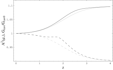
Figure 8: Reconstruction of the function $A(\varphi_{*})$ (top) and $V(\varphi_{*})$ (middle) of a scalar-tensor theory reproducing an equation of state of the form (10) with $z_{*}=0$, $w_{*}=-0.9$ and $w_{a}=1.2$ and a gravitational constant of the form (68) with $z_{G}=2$, $\delta z_{G}=1$ and $\Delta_{G}=0.1$ (solid) or $\Delta_{G}=-0.1$ (dash). We have assumed $\Omega_{{\rm m}0}=0.3$ and $\Omega_{K0}=0$. The lower plot compares $G_{\mathrm{cav}}(z)$ (black) to $A^{2}(z)$ (light).

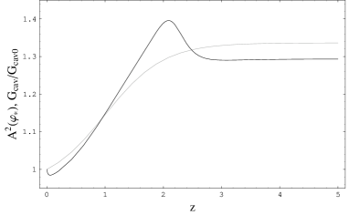
Figure 9: Reconstruction of the function $A(\varphi_{*})$ (top) and $V(\varphi_{*})$ (middle) of a scalar-tensor theory reproducing an equation of state of the form (10) with $z_{*}=0$, $w_{*}=-1.1$ and $w_{a}=1.6$ and a gravitational constant of the form (68) with $z_{G}=1$, $\delta z_{G}=1$ and $\Delta_{G}=0.4$. We have assumed $\Omega_{{\rm m}0}=0.3$ and $\Omega_{K0}=0$. The lower plot compares $G_{\mathrm{cav}}(z)$ (black) to $A^{2}(z)$ (light).

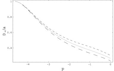
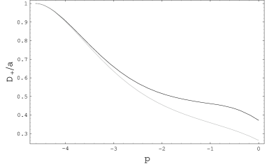
Figure 10: Comparaison of the growth factor of the scalar-tensor models with the models sharing same background dynamics but assuming general relativity. (top) Model depicted in Fig. 8 (long dash: $\Delta_{G}=-10\%$, short dash $\Delta_{G}=+10\%$, light curve: general relativity); (middle) Model depicted in Fig. 9 and (bottom) relative deviation.

IV.4 Class C vs class D

We have shown that the background dynamics of DGP models can be mimicked by a quintessence model, but that this was no more true at the perturbation level. It is obvious that a scalar-tensor theory that can reproduce a given $\{w(z),\beta(z)\}$ will mimick a DGP model, both for the background dynamics and perturbation evolution. Such a scalar-tensor theory, if it exists, will be characterized by

$$E(z)=E_{\rm DGP}(z),$$ (69)

$$\frac{G_{\mathrm{cav}}}{G_{\mathrm{cav}0}}=\frac{1+1/3\beta(z)}{1+1/3\beta(0)}\equiv g_{\rm DGP}(z).$$ (70)

In that case, the reconstruction procedure is the following. First, we can eliminate $U$ from Eq. (63) to get

$$\!\!\!\!\!\!\!\!\!\!\!\!\!\!\!\!Z\left(\frac{{\rm d}\varphi}{{\rm d}z}\right)^{2}=-\frac{{\rm d}^{2}F}{{\rm d}z^{2}}-\left[\frac{{\rm d}\ln E}{{\rm d}z}+\frac{2}{1+z}\right]\frac{{\rm d}F}{{\rm d}z}$$

$$+2\left[\frac{1}{1+z}\frac{{\rm d}\ln E}{{\rm d}z}-\frac{\Omega_{K0}}{E^{2}}\right]F-3\frac{1+z}{E^{2}}\Omega_{{\rm m}0}F_{0}.$$ (71)

This equation, together with Eq. (52), yields a non-linear second order differential equation for $F(z)$ with a source term given by Eq. (70).

Fig. 11 depicts the redshift evolution of the gravitational constant of the equivalent scalar-tensor theory (if it exists). Let us first stress that the time evolution of $G_{\mathrm{cav}}$ at $z=0$ varies a lot with the parameters of the DGP model. The constraint

$$\left|\frac{{\rm d}\ln G_{\mathrm{cav}}}{{\rm d}t}\right|_{0}<6\times 10^{-12}\,\rm{yr}^{-1}$$ (72)

implies that most DGP models, if interpreted as a scalar-tensor theory, are not compatible with Solar system experiments, since they should fulfill $|{\rm d}\ln G_{\mathrm{cav}}/{\rm d}z|_{0}<5.86\times 10^{-2}h^{-1}$. Fig. 11 summarizes the range of cosmological parameters of the DGP model for which the reconstructed scalar-tensor theory, if it exists, is compatible with Solar system tests on the time variation of the Newton constant.

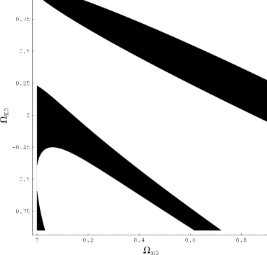
Figure 11: (top) $G_{\mathrm{cav}}(z)$ needed for a scalar-tensor theory to mimick a DGP model when $\Omega_{{\rm m}0}=0.3$ and $\Omega_{K0}=0$ (solid), $\Omega_{K0}=0.3$ (dashed) and $\Omega_{K0}=-0.3$ (dotted). (bottom): All DGP models which parameters are lying in the white zone do not fulfill the constraint (72) that will appear on the equivalent scalar-tensor theory.

The reconstruction is more easily performed by using the Brans-Dicke representation in which $F=\varphi$ and $Z=\omega(\varphi)/\varphi$ so that

$$G_{\mathrm{cav}}=\frac{G_{*}}{\varphi}\frac{2\omega+4}{2\omega+3}.$$ (73)

This representation is well-behaved in the sense that $\varphi^{\prime 2}$ remains positive and the energy condition reduces to $\omega\geq-3/2$. Using Eq. (73) to express $\omega$ as

$$2\omega=\frac{4-3\lambda_{0}g_{\rm DGP}(z)\varphi}{\lambda_{0}g_{\rm DGP}(z)\varphi-1}$$ (74)

with $\lambda_{0}=(2\omega_{0}+4)/(2\omega_{0}+3)$, Eq. (71) reduces to closed non-linear second order equation for $\varphi$. To performed the reconstruction, we need to determine $\varphi_{0}$, $\varphi^{\prime}_{0}$ and $\omega_{0}$. While it is always possible to set $\varphi_{0}=1$, we need to determine the two others. This can be done by using the expressions [76, 28, 77] of the PPN parameters

$$\gamma^{\mathrm{PPN}}-1 = -\frac{1}{\omega_{0}+2},$$ (75)

$$\beta^{\mathrm{PPN}}-1 = \frac{1}{4}\frac{1}{(2\omega_{0}+3)(\omega_{0}+2)^{2}}\frac{\omega_{0}^{\prime}}{\varphi_{0}^{\prime}}$$ (76)

and the expression of the time derivative of $G_{\mathrm{cav}}$ to get

$$\varphi^{\prime}_{0} = -\left(\frac{G^{\prime}_{\mathrm{cav}}}{G_{\mathrm{cav}}}\right)_{0}\left(1-4\frac{\beta^{\mathrm{PPN}}-1}{\gamma^{\mathrm{PPN}}-1}\right)^{-1}$$ (77)

$$\omega_{0} = -\left(\frac{1}{\gamma^{\mathrm{PPN}}-1}+2\right).$$ (78)

We see that the question of the reconstruction of the DGP cosmological dynamics by a scalar-tensor theory depends on the prediction of the DGP theory in the Solar system, an issue still not settled [81].

Table 1: Summary of the properties of the models considered here. We emphasize the predictions that one computes in these models (Y: yes, N: no, controversial: there is no current agreement at the moment).

model	class	background	Newtonian	cosmological	non-linear	Solar	strong	$w<-1$
			perturbations	perturbations	regime	system	field	possible
Quintessence	A	Y	Y	Y	almost	Y	Y	N
Scalar-tensor	C	Y	Y	Y	N	Y	Y	Y
DGP	D	Y	Y	controversial	N	controversial	Y	Y

Table 2: Summary of the comparisons performed in our exercices and of the possibility of two models to share the same predictions. (bgd=background; Newt. pert.= density perturbation in the Newtonian regime).

	bgd	bgd + Newt. pert.	bgd + Newt. pert. + Solar syst.
DGP vs quintessence	Y	N	N
DGP vs scalar-tensor	Y	?	N

Note that in Ref. [67], it was suggested that Eq. (45) implies that $\omega(z)=3[\beta(z)-1]/2$. Comparing with Eq. (73), this would mean that $G_{\mathrm{cav}}(0)$ is identified with $G_{*}/F_{0}$, which is the case only if $\omega_{0}\gg 1$ and that the redshift dependence of $\varphi$ is neglected. In such a case, one can check that $\omega<-3/2$ so that there is no hope to reconstruct a well-defined scalar-tensor theory. This may reflect the fact that the DGP model contains ghost modes around the self accelerating solution [82].

Playing with the parameters $\gamma^{\mathrm{PPN}}$ and $\beta^{\mathrm{PPN}}$, we can reconstruct well-defined scalar-tensor theories for some values. Indeed, there is no insurance at this stage that it really describes a DGP model. Anyway, it would mean that a DGP model and the scalar-tensor could share the same background and perturbation evolution. Of course, this does not mean that DGP-5D are scalar-tensor theories which would require a complete mapping of the degrees of freedom of each theory. Also, the two theories can be hoped to be discriminated by other features that are not discussed here such as the high-redshift properties (CMB, BBN), primordial predictions, strong field effects (black holes and gravitational waves emission) and, as discussed above and illustrated on Fig. 11, local test of gravity. While all these predictions are available for scalar-tensor theories, this is not yet the case for DGP models (see table 1).

V Conclusions

In this article, we have discussed various physical models of the dark energy sector that can be the cause of the acceleration of the universe, following a physically oriented classification relying on the nature and coupling of the degrees of freedom of dark energy as starting point. For each of the four classes, we have described specific signatures and tests (see Fig. 1).

Beside the evolution of the background, we insisted on the central role of the perturbations to distinguish between the four classes of models. Restricting to the Newtonian limit, we propose to characterize them by a new set of functions besides the equation of state. According to this classification scheme, the determination of the nature of dark energy can be outlined following a series of consistency checks in order to progressively exclude classes of models. Also, it can be used to quantify the departure from a pure $\Lambda$CDM in each class and to define target models in each class. Maybe it will just let us with the initial cosmological constant problem to face [10] after alternatives offered in the context of (well-defined) field theories have been exhausted. Let us recall that this analysis let a large class of solutions unexplored and also calls for tests of the Copernician principle.

As exercices, we have constructed models from different classes that share the same background dynamics and eventually the same growth history of density fluctuations (see table 2 for a summary). These models may be differentiated on the basis of local experiments, strong fields effects and of large scale perturbations (including CMB). This illustrates the importance of the theoretical prejudices when parameterizing the dark energy and the complementarity of data sets.

References

- [1] D.N. Spergel et al., [astro-ph/0603449].
- [2] M. Tegmark et al., Phys. Rev. D 69, 103501 (2004); S. Cole et al., Month. Not. R. Astron. Soc. 362, 505 (2005).
- [3] D. Eisenstein et al., Astrophys. J. 633, 560 (2005).
- [4] H. Hoekstra et al., [astro-ph/0511089].
- [5] E. Semboloni et al., [astro-ph/0511090].
- [6] P. Astier et al., [astro-ph/0510447 ]; A.G. Riess et al., Astrophys. J. 607, 665 (2004).
- [7] E. Copeland, M. Sami, and S. Tsujikawa, hep-th/0603057.
- [8] P. Peter and J.-P. Uzan, Cosmologie primordiale (Belin, 2005).
- [9] P.J.E. Peebles and B. Ratra, Rev. Mod. Phys. 75, 559 (2003).
- [10] T. Padmanabhan, [astro-ph/0603114].
- [11] R. Bean, S. Carroll, and M. Trodden, [astro-ph/0510059].
- [12] M. Tegmark, Phys. Rev. D66, 103507 (2002).
- [13] J.-P. Uzan, N. Aghanim, and Y. Mellier, Phys. Rev. D 70 083533 (2004).
- [14] J.-P. Uzan, Proc. of Phi in the Sky: The Quest of Cosmological Scalar Fields workshop (Porto), AIP Conf. Proceedings 736, 3 (2004); [astro-ph/0409424].
- [15] G. Lemaître, Ann. Soc. Sci. Bruxelles A 53, 51 (1933); R. Tolman, Proc. Natl. Acad. Sci. U.S.A. 20, 169 (1934); H. Bondi, Month. Not. R. Astron. Soc. 107, 410 (1947).
- [16] H. Iguchi, T. Nakamura, and K.-I. Nakao, Prog. Theor. Phys. 108, 809 (2002); H Alnes, M. Amarzguioui, and Ø. Grøn, [astro-ph/0506449]; R. Vanderveld, E. Flanagan, and I. Wasserman; [astro-ph/0602476]; M.-N. Célérier, Astron. Astrophys. 353, 63 (2000); K. Tomita, Month. Not. R. Astron. Soc. 326 287 (2001); K. Tomita, Prog. Theor. Phys. 106, 929 (2001).
- [17] R. Maartens and D. Matravers, Class. Quant. Grav. 11, 2693 (1994); N. Mustapha, C. Hellaby, and G.F.R. Ellis, Month. Not. R. Astron. Soc. 292, 817 (1997); G.F.R. Ellis, Quart. J. Astron. Soc. 16, 245 (1976).
- [18] G.F.R. Ellis, et al., Phys. Rep. 124, 315 (1985); O. Lahav, [astro-ph/0001061 ].
- [19] R. Rasanen, JCAP 0402, 003 (2004); R. Rasanen, JCAP 0411, 010 (2004); E.W. Kolb, S. Matarrese, and A. Riotto, [astro-ph/0506534]; M. Giovannini, JCAP 0509, 009 (2005); T. Buchert, Class. Quant. Grav. 22, L113 (2005). Y. Nambu and M. Tanimoto, [gr-qc/0507057]; A. Ishibashi and R. Wald,[gr-qc/0509108]; C.-H. Chuang, J.-A. Gu, and W-Y. Hwang, [astro-ph/0512651 ]; G.F.R. Ellis and T. Buchert, Phys. Lett. A 347, 38 (2005); C. Hirata and U. Seljak, Phys. Rev. D 72, 083501 (2005); E. R. Siegel and J. N. Fry, Astrophys. J. 628, L1 (2005); G. Geshnizjani, D. Chung, and N. Afshordi, Phys. Rev. D 72, 023517 (2005).
- [20] C. Wetterich, Nuc. Phys. B 302, 668 (1988); B. Ratra and J. Peebles, Phys. Rev. D 37, 321 (1988).
- [21] R. Battye, M. Bucher, and D. Spergel, astro-ph/9908407.
- [22] A. Sen, JHEP 9910, 008 (1999); A. Sen, JHEP 0204, 048 (2002); T. Padmanabhan, Phys. Rev. D 66, 021301 (2002).
- [23] A.Y. Kamenshchik, U. Moschella, and V. Pasquier, Phys. Lett. B 511, 265 (2001); M. Bento, O. Bertolami, and A. Sen, Phys. Rev. D 66, 043507 (2002).
- [24] T. Chiba, T. Okabe, and M. Yagamuchi, Phys. Rev. D 62, 023511 (2000); C. Armendariz-Picon, V. Mukhanov, and P. Steinhardt, Phys. Rev. Lett. 85, 103510 (2000).
- [25] C. Csaki, N. Kaloper, and J. Terning, Phys. Rev. Lett. 88, 161302 (2002); C. Deffayet et al., Phys. Rev. D 66, 043517 (2002); C. Deffayet and J.-P. Uzan, Phys. Rev. D 62, 063507 (2000).
- [26] B.A. Bassett and M. Kunz, Phys. Rev. D 69, 101305 (2004); Astrophys. J. 607, 661 (2004).
- [27] S. Srianand, P. Petitjean, and C. Ledoux, Nature 408 (2000) 931.
- [28] C.M. Will, Theory and experiment in gravitational physics, (Cambridge University Press, 1981).
- [29] R.P. Woodard, [astro-ph/0601672].
- [30] K. Stelle, Gen. Relat. Grav. 9, 353 (1978); A. Hindawi, B. Ovrut, and D. Waldram, Phys. Rev. D 53, 5583 (1996); E.T. Tomboulis, Physics Letter B 389, 225 (1996).
- [31] M. Ostrogradski, Mem. Ac. St. Petersbourgh VI-4, 385 (1850).
- [32] J.-P. Uzan, Phys. Rev. D 59 (1999) 123510; F. Perotta, C. Baccigalupi, S. Matarrese, Phys. Rev. D 61 (2000) 023507; A. Riazuelo and J.-P. Uzan, Phys. Rev. D 65 (2002) 043525; T. Chiba, Phys. Rev. D 60 (1999) 083508; L. Amendola, Phys. Rev. D 62 (2000) 043511; A. Riazuelo and J.-P. Uzan, Phys. Rev. D 62 (2000) 083506; L. Amendola, Phys. Rev. D 60 (1999) 043501.
- [33] J. Khoury and A. Weltman, Phys. Rev. Lett. 93, 171104 (2004).
- [34] J.-P. Uzan, Rev. Mod. Phys. 75 (2002) 403; J.-P. Uzan, Annales Henri Poincaré 4 (2003) 347; J.-P. Uzan, Int. J. Theor. Phys. 42, 1163 (2003).
- [35] C. Wetterich, Phys. Lett. B 561, 10 (2003).
- [36] T. Damour, F. Piazza, and G. Veneziano, Phys. Rev. Lett. 89, 081601 (2002).
- [37] J. Martin, C. Schimd, and J.-P. Uzan, Phys. Rev. Lett. 96, 061303 (2006).
- [38] B. Boisseau et al., Phys. Rev. Lett. 85, 2236 (2000).
- [39] T. Damour and C. Gundlach, Phys. Rev. Lett. 43, 3873 (1991).
- [40] R. Gregory, V. Rubakov, and S. Sibiryakov, Phys. Rev. Lett. 84, 4690 (2000).
- [41] I. Kogan et al., Nuc. Phys. B 584, 313 (2000); T. Damour and I. Kogan, Phys. Rev. D 66, 104024 (2002).
- [42] G. Dvali, G. Gabadadze, and M. Porati, Phys. Lett. B 485, 208 (2000); V. Sahni and Y. Shtanov, JCAP 0311 (2003) 014.
- [43] B. Carter et al., Class. Quant. Grav. 18, 4871 (2001); J.-P. Uzan, Int. J. Mod. Phys. A 17, 2739 (2002); J.-P. Uzan, Int. J. Theor. Phys. 41, 2299 (2002).
- [44] A. Amendola, Phys. Rev. Lett. 93, 181102 (2004).
- [45] F. Bernardeau, [astro-ph/0409224]; H.F. Stabenau and B. Jain, [astro-ph/0604038]; C. Sealfon, L. Verde, R. Jimenez, Phys. Rev. D 71, 083004 (2005); L. Amendola and C. Quercelini, Phys. Rev. Lett. 92, 181102 (2004).
- [46] C. Schimd et al.,[astro-ph/0603158].
- [47] A.R. Liddle, Month. Not. R. Astron. Soc. 351, L49 (2004); P. Mukherjee et al., [astr-ph/0512484].
- [48] C. Alcock and B. Paczynski, Nature 281 (1979) 358.
- [49] P. Teyssandier and P. Tourrenc, J. Math. Phys. 24, 2793 (1983).
- [50] S. Gottlöber, H.J. Schmidt, and A.A. Starobinsky, Class. Quant. Grav. 7, 893 (1990); D. Wands, Class. Quant. Grav. 11, 269 (1994).
- [51] M. Malquarti et al., Phys. Rev. D 67, 123503 (2003).
- [52] E.V. Linder and D. Huterer, Phys. Rev. D 72, 043509 (2005).
- [53] B. Basset, P. Corasaniti, and M. Kunz, Phys. Rev. D 69, 083517 (2004).
- [54] E.V. Linder and A. Jenkins, Month. Not. R. Astron. Soc. 346, 573 (2003).
- [55] E.V. Linder, Phys. Rev. D 72, 043529 (2005).
- [56] P.S. Corasaniti and E.J. Copeland, Phys. Rev. D 67, 063521 (2003).
- [57] B.A. Basset, et al., Month. Not. R. Astron. Soc. 336, 1217 (2002).
- [58] R. Dave, R. Caldwell, and P. Steinhardt, Phys. Rev. D 66, 023516 (2002).
- [59] M. Chevallier and D. Polarski, Int. J. Mod. Phys. D 10, 213 (2001).
- [60] E.V. Linder, Phys. Rev. Lett. 90, 091301 (2003).
- [61] W. Hu and B. Jain, Phys. Rev. D 70, 043009 2004).
- [62] E.V. Linder, [astro-ph/0604280].
- [63] R.R. Caldwell and E.V. Linder, Phys. Rev. Lett. 95, 141301 (2004).
- [64] R.J. Scherrer, [astro-ph/0509890].
- [65] J.-P. Uzan and F. Bernardeau, Phys. Rev. D. 64, 083004 (2001).
- [66] C. Schimd, J.-P. Uzan, and A. Riazuelo, Phys. Rev. D 71, 083512 (2005).
- [67] K. Koyama and R. Maartens, JCAP 0601, 016 (2006); K. Koyama, JCAP 0603, 017 (2006).
- [68] J.-P. Uzan and F. Bernardeau, Phys. Rev. D 63, 023004 (2000).
- [69] D. Sorkin, Int. J. Theor. Phys. 22, 1091 (1983); A.R. Liddle, Month. Not. R. Astron. Soc. 351, L49 (2004); J. Magueijo and D. Sorkin, [astro-ph/0604441].
- [70] B.A. Bassett, P.S. Corasaniti, and M. Kunz, Astrophys. J. 617, L1 (2004).
- [71] D.H. Weinberg, [astro-ph/0510196].
- [72] C. Deffayet, Phys. Lett. B 502, 199 (2001).
- [73] G.F.R. Ellis and M.S. Madsen, Class. Quantum Grav. 8, 667 (1991).
- [74] L. Knox, Y.S. Song and J.A. Tyson, [astro-ph/0503644]; I. Sawicki and S.M. Carroll, [astro-ph/0510364].
- [75] R. Maartens and E. Majerotto, [astro-ph/0603353]; Y.-S. Song [astro-ph/0602598].
- [76] T. Damour and G. Esposito-Farèse, Class. Quant. Grav. 9, 2093 (1992).
- [77] G. Esposito-Farèse and D. Polarski, Phys. Rev. D 63, 063504 (2001).
- [78] A. Coc, et al., [astro-ph/0601299].
- [79] L. Perivolaropoulos, JCAP 0510, 001 (2005); S. Nesseris and L. Perivolaropoulos, [astro-ph/0602053].
- [80] Z.K. Guo, N. Ohta, and Y.Z. Zhang, Phys. Rev. D 72, 023504 (2005).
- [81] A. Lue, Phys. Rep. 423, 1 (2006); A. Lue and G. Starkman, Phys. Rev. D67, 064002 (2003).
- [82] D. Gorbunov, K. Koyama, and S. Sibiryakov, Phys. Rev. D 73, 044016 (2006); A. Nicolis and R. Rattazzi, JHEP 0406, 059 (2004); K. Koyama, Phys. Rev. D 72, 123511 (2005).