Orbital elements, masses and distance of $\lambda$ Scorpii A and B determined with the Sydney University Stellar Interferometer and high resolution spectroscopy

Abstract

The triple system HD 158926 ($\lambda$ Sco) has been observed interferometrically with the Sydney University Stellar Interferometer and the elements of the wide orbit have been determined. These are significantly more accurate than the previous elements found spectroscopically. The inclination of the wide orbit is consistent with the inclination previously found for the orbit of the close companion. The wide orbit also has low eccentricity, suggesting that the three stars were formed at the same time.

The brightness ratio between the two B stars was also measured at $\lambda=$ 442 nm and 700 nm. The brightness ratio and colour index are consistent with the previous classification of $\lambda$ Sco A as B1.5 and $\lambda$ Sco B as B2. Evolutionary models show that the two stars lie on the main sequence. Since they have have the same age and luminosity class (IV) the mass-luminosity relation can be used to determine the mass ratio of the two stars: $M_{B}/M_{A}=0.76\pm 0.04$.

The spectroscopic data have been reanalyzed using the interferometric values for $P$, $T$, $e$ and $\omega$, leading to revised values for $a_{1}\sin i$ and the mass function. The individual masses can be found from the mass ratio, the mass function, spectrum synthesis and the requirement that the age of both components must be the same: $M_{A}=10.4\pm 1.3\,M_{\odot}$ and $M_{B}=8.1\pm 1.0\,M_{\odot}$.

The masses, angular semimajor axis and the period of the system can be used to determine the dynamical parallax. We find the distance to $\lambda$ Sco to be $112\pm 5$ pc, which is approximately a factor of two closer than the HIPPARCOS value of $216\pm 42$ pc.

1 Introduction

The bright southern star $\lambda$ Scorpii (HD 158926, HR 6527, $\alpha_{2000}=17^{\rm h}33^{\rm m}36\aas@@fstack{s}52$, $\delta_{2000}=-37^{\circ}06\arcmin 13\aas@@fstack{\prime\prime}8$, $V=1.62$) is classified as a B2IV+B single-lined spectroscopic binary system in the Bright Star Catalogue [Hoffleit & Warren 1991], but it is in fact a triple system. Two recent papers by Uytterhoeven and colleagues [Uytterhoeven et al. 2004a, Uytterhoeven et al. 2004b] present a detailed spectroscopic study of the system based on fourteen years of data. We shall refer to these as Papers I & II. These papers also include an extensive review of the literature on $\lambda$ Sco and here we present only a brief synopsis.

The system comprises two B stars of similar mass that orbit each other with a period of approximately 1000 days (the ‘wide’ system). The primary is a $\beta$ Cephei type variable with a low mass companion that orbits the primary with a period of 6 days (the ‘close’ system). The spectroscopic elements for the two orbits are given in Paper I. The close binary system is eclipsing and in Paper I it is shown that this constrains the inclination to the range $70^{\circ}<i_{\rm close}<90^{\circ}$. An independent argument in Paper II based on frequency analysis also gives the same result.

Paper II notes that the wide orbit cannot be accurately determined from the spectroscopy. We report here interferometric observations made with the Sydney University Stellar Interferometer (SUSI) on the wide system that results in a much improved orbit.

In Section 2 we present the SUSI observations and the new interferometric orbit.

In Section 3 the interferometric elements are used to determine a revised spectroscopic orbit. Interferometry also provides the brightness ratio between the distant component and the primary. The mass-luminosity relation can be used to find the mass ratio, and using the spectroscopically determined mass function, the individual masses can be calculated. Having determined the masses the dynamical parallax for $\lambda$ Sco can be calculated. It differs significantly from the HIPPARCOS parallax.

Following Papers I & II we use ‘close’ and ‘wide’ to distinguish the orbital elements associated with the 6-day and 1000-day periods seen in the spectrum of the primary. When no subscript is used the wide system is implied.

In the case of the interferometric data we follow the scheme proposed in the Washington Multiplicity Catalog (WMC) [Hartkopf & Mason 2003]. The primary will be denoted by ‘A’, the close companion by ‘a’ and the wide component by ‘B’. The notation $a_{Aa}$, for example, denotes the semimajor axis of the orbit of a relative to the primary while $a_{Aa,B}$ is the semimajor axis of B relative to the centre of light of the close pair.

2 The SUSI observations and the interferometric orbit

2.1 Observations with the ‘blue’ beam-combining optics

Observations prior to 2004 were made at the blue wavelength of 442 nm using a bandwidth of 4 nm. The optical layout was essentially the same as the one described in Davis et al. [Davis et al. 1999]. The data were reduced using the same procedure that was employed for the analysis of the binary system $\beta$ Cen [Davis et al. 2005a].

Baselines of 5, 10 and 20 metres were used. For these baselines the two B stars are essentially unresolved by SUSI. Because of atmospheric turbulence the fringe phase carries no useful information, and SUSI, like most optical interferometers, measures a quantity proportional to the squared modulus of the complex degree of coherence $\gamma$:

$$|\gamma|^{2}=\frac{1+\beta^{2}+2\beta\cos(2\pi{\bf b}\!\cdot\!\mn@boldsymbol{\rho}/\lambda)}{(1+\beta)^{2}}$$ (1)

where $\bf b$ is the projected baseline, $\mn@boldsymbol{\rho}$ is the vector separation between the two components of the binary as seen from the Earth and $\beta=I_{B}/I_{A}\leq 1$ is the brightness ratio.

The SUSI data taken with the blue beam-combining system are ‘uncalibrated’; i.e., no unresolved reference stars were observed to take into account the reduction in the observed fringe signal due to atmospheric and instrumental effects. The seeing conditions vary during the night, and experience has shown that modelling this by a simple linear time variation is usually adequate. We therefore assume that the observed signal will have the form

$$|V|^{2}=(C_{a}-C_{b}t)|\gamma|^{2}$$ (2)

where $t$ is the hour angle of $\lambda$ Sco. The two empirical factors $C_{a}$ and $C_{b}$ are free parameters in the model fitting procedure. The sign in equation (2) reflects the fact that in general the seeing deteriorates during the night.

It should be noted that the cosine term in equation (1) depends on the position angle $\theta$ and the separation $\rho$. When the raw $|V|^{2}$ data are fitted using equation (2) the resultant estimates for $\rho$ and $\theta$ are not significantly affected by the fact that the data are uncalibrated. The estimate for the brightness ratio, on the other hand, may be subject to systematic errors.

The presence of a cosine in equation (1) means that there is a $180^{\circ}$ ambiguity in the position angle (a two-aperture interferometer cannot distinguish between $\mn@boldsymbol{\rho}$ and $-\mn@boldsymbol{\rho}$). This has no impact on the interpretation of the results presented here.

Equation (1) does not take into account the presence of the close binary orbiting the primary. However, Paper I notes that the contribution of H_α emission from weak T Tauri stars is at least 2 orders of magnitude fainter than the primary. Modulation due to the faint companion will be at most 1% and generally much smaller than this. This is less than the measurement noise and consequently the effect of the T Tauri component on the interferometric data will be negligible.

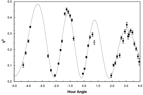
Figure 1: A typical set of data from one night (27 June 2000). Each point represents a measurement of $|V|^{2}$. The data are fitted using equation (2) and the best fit is shown. The error bars denote the formal errors of the data points. The actual uncertainties are estimated to be 2.8 times larger. The point shown as an open circle was omitted from the final fit.

The binary star measures were estimated from the $|V|^{2}$ data using essentially the same procedure described by Davis et al. [Davis et al. 2005a]. The data from each night were fitted using equation (2) and the data for a typical night are shown in Fig. 1. The formal error for each data point in general underestimates the actual scatter because the seeing varies throughout the night. Having found the best fit to the data the formal errors are rescaled to make $\chi^{2}=\nu$, where $\chi^{2}$ is the weighted sum of the squared residuals and $\nu$ is the number of degrees of freedom. In effect, we assume that the actual uncertainties obey Gaussian statistics and all the data points are similarly affected by seeing (in the example shown in Fig. 1 the scaling factor was 2.8). Using the rescaled weighting factors Monte Carlo simulation is then used to determine the uncertainties in the fitting parameters.

The assumption that all the points are equally affected by seeing is not strictly true, but if the seeing does not change dramatically during the night this assumption is, on average, realistic. The seeing is continually measured and logged, and points that are badly affected by seeing are excluded from the final fit.

A completely independent analysis was performed using simulated annealing [Kirkpatrick et al. 1983]. Simulated annealing is more likely to converge on the true minimum of $\chi^{2}$ rather than on a local minimum, unlike steepest descent methods. The simulated annealing results did not differ significantly from those obtained by our standard method and we are confident that the values of $\rho$, $\theta$ and $\beta$ and their uncertainties that are given in Table 1 are the best fit to each night’s data. The separation $\rho$ and related quantities are all expressed in milliarcseconds (mas).

Table 1: The binary star measures determined with SUSI. The date, Julian date, the baseline used and the wavelength are tabulated along with the measured values of $\rho$, $\theta$, $\beta$ and their uncertainties. The weighting factor $W$ was used when fitting the orbit and is a measure of the accuracy of each point. The final column gives the residual between the observed data and the position calculated from the best fitting model. Using the WMC nomenclature, all these observations are classified as Aa,B.

Date	JD	$B$	$\lambda$	$\Delta\lambda$	$\rho$	$\sigma_{\rho}$	$\theta$	$\sigma_{\theta}$	$\beta$		$\sigma_{\beta}$	$W$	$|O-C|$
(UT)		(m)	(nm)	(nm)	(mas)	(mas)						(mas-1)	(mas)
1999-05-15	2451314.1	10	442	4	45.86	0.19	265 $\aas@@fstack{\circ}$92	0 $\aas@@fstack{\circ}$06	0.532		0.008	5.0	0.51
1999-05-17	2451316.1	5	442	4	45.66	0.27	266 $\aas@@fstack{\circ}$37	0 $\aas@@fstack{\circ}$08	0.596		0.009	3.6	0.44
1999-06-04	2451334.1	5	442	4	46.12	0.18	267 $\aas@@fstack{\circ}$95	0 $\aas@@fstack{\circ}$07	0.649		0.009	5.2	0.73
1999-06-22	2451352.1	5	442	4	46.79	0.97	268 $\aas@@fstack{\circ}$93	0 $\aas@@fstack{\circ}$27	0.540		0.013	1.0	0.50
1999-06-23	2451353.1	5	442	4	46.25	0.83	268 $\aas@@fstack{\circ}$50	0 $\aas@@fstack{\circ}$26	0.580		0.023	1.2	1.11
1999-08-12	2451403.1	5	442	4	44.53	1.82	273 $\aas@@fstack{\circ}$09	0 $\aas@@fstack{\circ}$43	0.482		0.020	0.5	1.40
2000-05-11	2451676.1	10	442	4	25.73	0.21	72 $\aas@@fstack{\circ}$46	0 $\aas@@fstack{\circ}$19	0.553		0.015	4.5	0.34
2000-05-12	2451677.1	10	442	4	26.08	0.14	72 $\aas@@fstack{\circ}$73	0 $\aas@@fstack{\circ}$10	0.596		0.006	6.6	0.29
2000-05-15	2451680.1	10	442	4	26.96	0.16	73 $\aas@@fstack{\circ}$95	0 $\aas@@fstack{\circ}$11	0.590		0.019	5.9	0.16
2000-05-18	2451683.1	10	442	4	28.33	0.11	74 $\aas@@fstack{\circ}$74	0 $\aas@@fstack{\circ}$09	0.609		0.003	8.4	0.52
2000-05-27	2451692.1	10	442	4	30.23	0.23	76 $\aas@@fstack{\circ}$49	0 $\aas@@fstack{\circ}$19	0.537		0.010	4.0	0.18
2000-06-02	2451698.1	10	442	4	31.43	0.14	77 $\aas@@fstack{\circ}$56	0 $\aas@@fstack{\circ}$13	0.528		0.005	6.4	0.06
2000-06-03	2451699.1	10	442	4	31.45	0.10	77 $\aas@@fstack{\circ}$57	0 $\aas@@fstack{\circ}$07	0.600		0.002	9.0	0.29
2000-06-04	2451700.1	10	442	4	31.25	0.10	77 $\aas@@fstack{\circ}$72	0 $\aas@@fstack{\circ}$05	0.575		0.005	10.0	0.72
2000-06-07	2451703.1	10	442	4	32.41	0.13	78 $\aas@@fstack{\circ}$35	0 $\aas@@fstack{\circ}$06	0.529		0.008	7.3	0.26
2000-06-11	2451707.1	10	442	4	33.45	0.28	78 $\aas@@fstack{\circ}$83	0 $\aas@@fstack{\circ}$14	0.468		0.008	3.4	0.21
2000-06-27	2451723.1	10	442	4	36.94	0.14	81 $\aas@@fstack{\circ}$39	0 $\aas@@fstack{\circ}$07	0.613		0.014	6.7	0.10
2000-06-30	2451726.1	10	442	4	37.44	0.24	81 $\aas@@fstack{\circ}$83	0 $\aas@@fstack{\circ}$14	0.455		0.010	3.9	0.20
2000-07-01	2451727.1	5	442	4	40.00	0.40	82 $\aas@@fstack{\circ}$08	0 $\aas@@fstack{\circ}$18	0.588		0.014	2.4	2.16
2000-07-22	2451748.1	5	442	4	43.54	0.21	84 $\aas@@fstack{\circ}$10	0 $\aas@@fstack{\circ}$09	0.560		0.009	4.4	1.83
2000-08-02	2451759.1	5	442	4	44.30	0.26	85 $\aas@@fstack{\circ}$30	0 $\aas@@fstack{\circ}$16	0.543		0.012	3.5	0.83
2001-06-22	2452083.1	10	442	4	18.80	0.17	129 $\aas@@fstack{\circ}$16	0 $\aas@@fstack{\circ}$43	0.534		0.012	4.5	1.14
2001-08-10	2452132.1	10	442	4	12.97	0.16	163 $\aas@@fstack{\circ}$25	1 $\aas@@fstack{\circ}$61	0.563		0.018	2.5	0.62
2001-08-19	2452141.1	20	442	4	12.58	0.04	174 $\aas@@fstack{\circ}$46	0 $\aas@@fstack{\circ}$43	0.476		0.009	9.6	0.54
2004-04-15	2453111.2	20	700	80	24.05	0.20	118 $\aas@@fstack{\circ}$92	0 $\aas@@fstack{\circ}$24	0.544		0.001	4.5	0.69
2004-04-20	2453116.2	20	700	80	23.38	0.24	119 $\aas@@fstack{\circ}$37	0 $\aas@@fstack{\circ}$51	0.518	a	0.028	3.1	0.34
2004-06-24	2453181.0	20	700	80	12.77	0.03	160 $\aas@@fstack{\circ}$40	0 $\aas@@fstack{\circ}$30	0.488		0.006	13.3	0.26
2005-04-17	2453478.2	20	700	80	47.42	0.20	270 $\aas@@fstack{\circ}$36	0 $\aas@@fstack{\circ}$05	0.516		0.014	4.8	0.18
2005-07-18	2453570.0	15	700	80	37.83	0.37	279 $\aas@@fstack{\circ}$45	0 $\aas@@fstack{\circ}$10	0.635	a	0.019	2.6	0.17
2005-07-21	2453573.0	15	700	80	37.18	0.23	279 $\aas@@fstack{\circ}$76	0 $\aas@@fstack{\circ}$05	0.536	a	0.013	4.2	0.24
2005-08-17	2453600.0	15	700	80	32.23	0.28	283 $\aas@@fstack{\circ}$68	0 $\aas@@fstack{\circ}$07	0.543	a	0.008	3.5	0.45

^a $V^{2}_{\rm max}<1$ for these sets of data. The other observations at 700 nm were fitted using $|V|^{2}=1$. This is discussed in Section 2.2.

2.2 Observations with the ‘red’ beam-combining optics

The more recent SUSI data have been obtained with the red beam-combining optics. This system has been described in Davis et al. [Davis et al. 2005b]. The observations were made using baselines in the range 10–20 metres. Again the individual B stars are unresolved at these baselines and the effect of the six-day companion on the data will be negligible.

The red observations were made at $\lambda=700$ nm using a bandwidth of 80 nm. With such a wide bandwidth the effects of “bandwidth smearing” cannot be ignored. Tango & Davis [Tango & Davis 2002] have discussed bandwidth smearing in the context of single stars and it is straightforward to generalize their results to arbitrary systems. In particular, if $\nu=c/\lambda$ is the optical frequency, $S_{\nu}$ is the spectral response of the interferometer and

$$N_{\nu}=\int\!\!\!\int\!d^{2}\mathbf{x}I_{\nu}(\mathbf{x})$$ (3)

is the integrated monochromatic flux from the source (the integral is taken over the plane of the sky), the broad band complex degree of coherence will be

$$\overline{\gamma}=\frac{\int_{0}^{\infty}d\nu S_{\nu}N_{\nu}\gamma(\nu)}{\int_{0}^{\infty}d\nu S_{\nu}N_{\nu}}$$ (4)

where $\gamma(\nu)$ is the quasimonochromatic complex degree of coherence defined by

$$\gamma(\nu)=N_{\nu}^{-1}\int\!\!\!\int\!d^{2}\mathbf{x}\exp\{-2\pi i\mathbf{b\!\cdot\!x}c^{-1}\nu\}I_{\nu}(\mathbf{x})$$ (5)

The complex coherence $\gamma(\nu)$ will vary with frequency (a) because of the frequency dependence of the Fourier kernel and (b) because $I_{\nu}({\mathbf{x}})/N_{\nu}$ is also a function of the frequency. In the case of a binary system with unresolved components this latter effect will be unimportant.

We assume that the bandwidth is rectangular, having a width $\delta\nu$ centred on $\nu_{0}$. Let $\lambda_{0}=c/\nu_{0}$ and make the usual approximation that $\delta\nu\approx c\delta\lambda/\lambda_{0}^{2}$. For convenience define $\psi=2\pi{\bf b}\!\cdot\!\mn@boldsymbol{\rho}/\lambda_{0}$. The equivalent of equation (1) including bandwidth smearing becomes:

$$|\gamma|^{2}=\!\frac{1+\beta^{2}{\rm\;sinc}^{2}(\psi\delta\lambda/2\lambda_{0})+2\beta{\rm\;sinc}(\psi\delta\lambda/2\lambda_{0})\cos\psi}{(1+\beta)^{2}}$$ (6)

In the case of $\lambda$ Sco the effect of bandwidth smearing can reduce $|\gamma|^{2}$ by several percent. The effect is time-dependent, and is most significant when $\bf b$ and $\mn@boldsymbol{\rho}$ are parallel.

The red table observations were first processed using the “data pipeline” described in Davis et al. [Davis et al. 2005b]. The output is a set of calibrated measures of $|V|^{2}$. The visibility measures for each night were fitted using the same procedure adopted for the ‘blue’ observations. The only difference is that the red data are fitted using equation (6) rather than equation (2). The most noticeable difference between the blue and red data sets is that the errors in the red data points required very much less rescaling, confirming the fact that the use of calibrators significantly reduces the effects of seeing on the data.

If the data are properly calibrated the maximum value of $|V|^{2}$, $|V|^{2}_{\rm max}$, should be 1. On several nights, however, it was found that allowing $|V|^{2}_{\rm max}$ to be a free parameter gave significantly better fits, with $|V|^{2}_{\rm max}<1$. The reduction cannot be explained by the partial resolution of the B stars or the modulation caused by the 6-day close companion. We believe that the effect is most likely instrumental but there are as yet not enough data to establish the exact cause. This effect has a negligible effect on the values of $\rho$ and $\theta$, but may affect $\beta$.

The results from the observations made with the red beam-combining system are given in Table 1.

2.3 The interferometric orbit

Figure 2: The orbit of $\lambda$ Sco. The scale is in millarcsec and the orientation conforms to standard practice [Heintz 1978]. Different symbols are used to denote successive orbits, referred to the epoch of periastron $T$. The circles indicate data taken in 1999. The triangles are the data from 2000 and 2001. The diamonds denote points on the next orbit during 2004 and 2005. Open symbols are used for observations at 442 nm; filled symbols denote 700 nm observations.

The orbital elements were calculated, again using the same procedure that was employed for $\beta$ Cen [Davis et al. 2005a]. Each measure in Table 1 was given a weight according to the formula: $W=(\sigma_{\rho}^{2}+\rho^{2}\sigma_{\theta}^{2})^{-1/2}$. The results are given in Table 2, and the ‘$|O-C|$’ residuals are tabulated in Table 1.

The uncertainties in the orbital elements were estimated using Monte Carlo simulation using the best fit orbital elements and the weighting factors in Table 1 to generate the simulated data sets. The resultant uncertainties are also listed in Table 2.

The period $P$, epoch of periastron $T$ and eccentricity $e$ differ significantly from those given in Paper I (see Table 3), and we return to this in Section 3.

The computed orbit and the observed measures are shown in Fig. 2. This figure also confirms the fact that any effects caused by the close companion must be smaller than the fitting errors.

Table 2: The orbital elements of $\lambda$ Sco determined from the SUSI observations. All the elements refer to the Aa,B orbit.

Element	Value, uncertainty and units
$P$	1052.8$\;\pm\;$	1.2	d
$T$	51 562.3$\;\pm\;$	2.8	MJD
$e$	0.121$\;\pm\;$	0.005
$a\arcsec$	49.3$\;\pm\;$	0.3	mas
$i$	77$\aas@@fstack{\circ}$2$\;\pm\;$	0$\aas@@fstack{\circ}$2
$\omega$	74$\aas@@fstack{\circ}$8$\;\pm\;$	0$\aas@@fstack{\circ}$9	See note.
$\Omega$	271$\aas@@fstack{\circ}$30$\;\pm\;$	0$\aas@@fstack{\circ}$15
$(a\arcsec)^{3}/P^{2}$	$(108\pm 2)\times 10^{-12}$		asec3d-2

Note:  This is the argument of periastron for the orbit of the B component relative to the primary. The corresponding quantity in Table 3 refers to the orbit of the primary around the system barycentre. The two angles differ by 180^∘.

Our value of the inclination, $i_{Aa,B}=77\aas@@fstack{\circ}2\pm 0\aas@@fstack{\circ}2$, is completely consistent with the range $70^{\circ}\leq i_{\rm close}\leq 90^{\circ}$ given in Papers I & II and, together with the relatively low eccentricity of the interferometric orbit, supports the hypothesis that the $B$ component did not join the system as a result of a tidal capture event.

2.4 The brightness ratio and the mass ratio

Figure 3: The brightness ratios, taken from Table 1. The two lines denote the range in $\beta$ that is expected due to the intrinsic variability of the system. The data prior to JD 2 452 500 were measured at $\lambda=442$ nm. The more recent data were measured at 700 nm.

For the reasons discussed in Section 2.1 the brightness ratio $\beta$ is subject to systematic errors associated with the way the $|V|^{2}$ data are normalized. As well, the system is a $\beta$ Cephei variable with a photometric amplitude in $v$ of approximately 0.023 magnitudes and a period of 5$\aas@@fstack{h}$1. [Shobbrook & Lomb 1972, Shobbrook & Lomb 1975].

Shobbrook & Lomb [Shobbrook & Lomb 1975] also observed periodic variations in colour. The amplitudes of the variation were $(b-v)=0.002\pm 0.001$ and $(u-b)=0.0098\pm 0.0012$.

The measured brightness ratios and their uncertainties are plotted in Fig. 3. The data fall into two groups: the earlier set of points were observed using $\lambda=442$ nm while the more recent set was obtained using $\lambda=700$ nm. The two lines represent the approximate spread in $\beta$ that would be expected from the intrinsic variability ($\sim\!\pm 0.012$ mag). The error bars indicate the statistical uncertainties for each observation, but in the present context they are misleading, since there are significant night-to-night variations due to the intrinsic variability of $\lambda$ Sco as well as the instrumental effects (calibration errors) previously discussed. In our view the average and standard error of the blue and red data sets represent the best estimates of the brightness ratios.

The means and standard deviations for the brightness ratio for each set, and the corresponding magnitude differences, are

$$\beta_{442}=0.55\pm 0.05 \Delta m_{442}=0.65\pm 0.10$$ (7)

$$\beta_{700}=0.54\pm 0.05 \Delta m_{700}=0.67\pm 0.10$$ (8)

The difference in the colour index $(m_{442}-m_{700})$ between $\lambda$ Sco A and B is $-0.02\pm 0.14$. Both the magnitude and colour index differences are consistent with the relative spectral classification of $\lambda$ Sco A as B1.5 IV and $\lambda$ Sco B as B2 V given in Paper I.

Although the A and B components have apparently different luminosities, due to the complexity of this system and the fast rotation there is an uncertainty of up to 0.2 dex in $\log g$, making it difficult to establish the luminosity class with certainty. However, the inclination of the long period orbit suggests that the three stars formed together and $\lambda$ Sco A and B are thus both on the main sequence. The brightness ratio then implies that the effective temperatures can be fixed at 25 000 K and 21 000 K. The contribution of the T Tauri star to the luminosity of the primary is negligible and the empirical mass-luminosity relation $\log(L_{B}/L_{A})=(3.51\pm 0.14)\log(M_{B}/M_{A})$ [Griffiths et al. 1988] can be used to find the mass ratio for $\lambda$ Sco A and B. The ratio of the luminosities has been obtained from the V magnitude difference, taken to be 0.66$\pm$0.10 by interpolation between $\Delta m_{442}$ and $\Delta m_{700}$, and the difference in bolometric correction (BC). The latter has been obtained from interpolation in the tables by Flower [Flower 1996] for main-sequence B stars. Assuming an uncertainty of $\pm$1000 K in the effective temperatures as obtained in Paper I, we arrive at (BC_A - BC_B) = -0.40$\pm$0.10. Thus the mass ratio for $\lambda$ Sco A and B is:

$$\frac{M_{B}}{M_{A}}=0.76\pm 0.04$$ (9)

This is consistent with the value of $M_{B}/M_{A}=0.84\pm 0.12$ estimated from the spectrum synthesis analysis presented in Paper I.

3 The combined interferometric and spectroscopic orbit

Figure 4: The radial velocity data for the ‘wide’ system in $\lambda$ Sco. The RV due to the ‘close’ system has been removed. In the upper panel the data are plotted against the FOTEL phase and the RV curve is calculated from the FOTEL elements in Table (3). The same RV data are plotted in the lower panel against the SUSI phase, with the RV curve calculated using the elements given in the final column of Table (3).

The spectroscopic orbital elements were determined in Paper I using two different codes, FOTEL and VCURVE. The upper panel of Fig. 4 plots the RV data against the FOTEL phase. The solid line is the calculated RV using the FOTEL elements (this panel is the same as the lower panel in Fig. 2 of Paper I).

The interferometric values for $P$, $T$, $e$ and $\omega$ are much more accurate than the spectroscopically determined ones, and the original RV data were refitted using these values, giving $K_{\rm wide}=22.8\pm 0.4$ km$\cdot$s^-1. Table 3 tabulates the elements given in Paper I and our revised values, and the RV amplitude calculated using these elements is shown in the lower panel of Fig. 4.

Table 3: The second column lists the elements found in Paper I using the FOTEL code. The third column tabulates the elements used in the final fit: $P$, $T$, $e$ and $\omega$ are based on the SUSI; $K$ has been recomputed using these values. The uncertainties are the formal uncertainties of the fit and do not include systematic effects.

Element	FOTEL		FOTEL+SUSI
$P$ (d)	1082$\,\pm\,$	3	1052.8$\,\pm\,$	1.2
$K$ (km$\cdot$s-1)	24.7$\,\pm\,$	0.4	22.8$\,\pm\,$	0.4
$T$ (MJD)	51 731.5$\,\pm\,$	29	51 562.3$\,\pm\,$	2.8
$e$	0.23$\,\pm\,$	0.03	0.121$\,\pm\,$	0.005
$\omega$	311∘$\,\pm\,$	11∘	254$\aas@@fstack{\circ}$8$\,\pm\,$	0$\aas@@fstack{\circ}$9

Some words of caution on the accuracy of the RV data are in order. The use of two types of spectra of very different nature and quality forced the authors of Paper I to use different methodology to derive the RV values. In doing so, they ignored the fact that the B component contributes to the spectral lines used for the RV computation, given that the binary is observed to be single-lined. The light, and hence mass ratio, found from the interferometry is an order of magnitude more precise than the one in Paper I and thus allows us to place better constraints on the individual masses of the A and B components. The ranges listed in Paper I must be revised, as they do not include the systematic effects due to the B component on the spectral lines used to determine the amplitude of the RV.

To make the best use of the interferometric results it is important to understand the uncertainties and possible systematic effects in the RV data. In general, the contribution of the B component to the lines leads to an underestimation of the RV of the primary. As a consequence, the derived quantities $a\sin i$ and the mass function are also underestimated. This fact was clearly demonstrated and corrected for by spectral disentangling in the case of the double-lined binary $\beta$ Cen [Ausseloos 2006], where it implied a 10% increase in the individual component masses. We are unable to apply such a treatment to $\lambda$ Sco because the disentangling fails in this single-lined case with three stellar components, of which at least one is oscillating (see Paper II). Nevertheless, we can estimate the systematic errors of the RVs for the two sets of data from which they were derived:

1. the high S/N single-order spectra including the Si iii 4553Å line taken with CAT/CES;

2. the low S/N échelle spectra taken with Euler/CORALIE.

The resolution for both sets of data is nearly the same (see Paper I for details).

From set (i) we derive that the lines due to the B component are completely situated within those of the primary (see Paper I and Waelkens [Waelkens 1990] for appropriate plots of the lines). Moreover, from the brightness ratio and the temperature ranges listed in Paper I we derive that the $\lambda$ Sco B contributes 40% to the total equivalent width of the Si iii line used to determine the RVs. This places strong constraints on the upper limit to $K_{\rm wide}$: the fact that the B component is not seen in the wings of the high-quality CAT profiles implies that $K_{\rm wide}<25.7$ km$\cdot$s^-1 (which we deduce from merging the contributions of the two stars to the Si iii line with the appropriate EW ratios and $v\sin i$ estimates of Papers I and II). This suggests a conservative range for $K_{\rm wide}$ is $[22.4,25.7]$ km$\cdot$s^-1. Table 4 tabulates the system parameters that are affected by the uncertainties in the radial velocity amplitude. The accurate value of the mass ratio given in equation (9) has been used to calculate the individual masses from the mass function.

Table 4: System parameters that depend on the RV amplitude. The lower limit for $K_{\rm wide}$ is taken from Table 3. The upper limit is based on our best estimates of the effects of the wide component on the RV data and from the interferometric data.

Element	Range
$K_{\rm wide}$	[22.4, 25.7]	km$\cdot$s-1
$a_{1}\sin i_{\rm wide}$	[2.15, 2.47]	AU
$a_{1}$	[2.21, 2.53]	AU
$f(M)$	[1.20, 1.82]	M⊙
$M_{A}$	[9.39, 14.25]	M⊙
$M_{B}$	[7.05, 10.69]	M⊙

The mass ranges listed in Table 4, although compatible with those given in Paper I, are very broad. We tried to constrain them further by taking into account the results from the spectrum synthesis presented in Paper I, in which the contributions from the individual components were properly taken into account to fit H, He, and Si lines in data set (ii). We did this by scanning the data base of standard stellar evolution models computed by Ausseloos et al. [Ausseloos et al. 2004]. We selected models from the ZAMS to the TAMS with $X=0.70$ and $Z$ in the range 0.012 to 0.030. Models with the three values 0.0, 0.1 and 0.2 for the core overshooting parameter (expressed in units of the local pressure scale height) were included. While scanning the database, we required that the two stars not only satisfy the mass ranges given in Table 4, but also that they have the appropriate luminosity ratio given by the interferometry, and have $\log T_{\rm eff}$ and $\log g$ in the ranges found from the spectrum synthesis done in Paper I. Moreover, we required that their ages be the same to within 0.1% (following the interferometric result that the orbital inclinations of the A and B components are consistent with each other). In this way, we find the acceptable range for the mass of the primary $M_{A}$ to be $[9.0,11.7]\,M_{\odot}$ and the range for $M_{B}$ to be $[7.0,9.1]\,M_{\odot}$.

All the acceptable model combinations at the lower mass ends of these intervals have an age below $10^{7}$ yr corresponding to less than 60% of the main sequence lifetime, while those at the upper mass end correspond to an age below $13\times 10^{7}$ yr which is less than 30% of the main sequence duration. For the lower mass end, this is consistent with the suggestion made in Paper I that $\lambda$ Sco contains a pre-MS star. Indeed, from Palla & Stahler [Palla & Stahler 1993] we note that a pre-MS star with a mass of $\sim 1.5\,M_{\odot}$ remains about $10^{7}$ yr in its pre-MS stage when a B-type star formed from the same accretion disk has reached the ZAMS. Table 5 summarizes our conclusions regarding the three components of $\lambda$ Sco.

Table 5: Summary of the stellar parameters of the three compoents of $\lambda$ Sco. The mass of the a component is taken from Paper I; the masses of $\lambda$ Sco A and B are based on the work presented here (compare with Table 4 of Paper I).

	Mass ($M_{\odot}$)	$T_{\rm eff}$ (K)	$\log g$
A	$10.4\pm 1.3$	$25\,000\pm 1\,000$	$3.8\pm 0.1$	B1.5 IV
a	$1.8\pm 0.2$			pre-MS
B	$8.1\pm 1.0$	$21\,000\pm 1\,000$	$4.0\pm 0.1$	B2 IV

3.1 The dynamical parallax

The dynamical parallax is

$$\pi_{d}=\frac{365.25^{2/3}}{(M_{Aa}+M_{B})^{1/3}}\left[\frac{(a\arcsec)^{3}}{P^{2}}\right]^{1/3}$$ (10)

where $M_{Aa}$ is the combined mass of the primary (A) and the close companion (a) and $M_{B}$ the mass of the B component. We have used the estimates given in Table 5 and the interferometric value of $(a\arcsec)^{3}/P^{2}$ (Table 2) to find the distance to $\lambda$ Sco:

$$D=1/\pi_{d}=112\pm 5~{}{\rm pc}$$ (11)

Our distance is smaller than the HIPPARCOS value of $216\pm 42$ pc [Perryman et al. 1997] by nearly a factor of two (i.e., 2.5 times the HIPPARCOS standard deviation). It has been noted [de Zeeuw et al. 1999] that the motion in binary systems can significantly bias HIPPARCOS parallaxes and a similar phenomenon has been observed with $\beta$ Cen [Davis et al. 2005a].

The revised parallax may have implications regarding the membership of $\lambda$ Sco in the Scorpius-Centaurus-Lupus-Crux complex of OB associations. Brown & Verscheuren [Brown & Verschueren 1997] suggested that it was a member of the Upper Scorpius (US) association, but de Zeeuw et al. [de Zeeuw et al. 1999] did not include $\lambda$ Sco as a secure member of the US association based on an analysis of HIPPARCOS positions, parallaxes and proper motions. The revised parallax corresponds to the Lower Centaurus Crux (LCC) association, which lies at a distance of $116\pm 2$ pc. The galactic coordinates of $\lambda$ Sco, however, still exclude it as a definite member of the association.

4 Summary

Observations with SUSI have been used to establish an interferometric orbit for $\lambda$ Sco. The accuracy of the period, epoch of periastron, eccentricity and argument of periastron are significantly better than those previously found (Paper I). We have combined the interferometric and spectroscopic elements to provide an orbital solution which is consistent with both the interferometric and spectroscopic data. The inclination of the orbit for the wide component is consistent with that previously found for the close companion, and the eccentricity of its orbit is quite low. This is strong evidence that the system was formed from a common accretion disk rather than through tidal capture.

The brightness ratio allows the mass ratio of the two B stars to be estimated from the mass-luminosity relation. The estimated mass ratio of $0.76\pm 0.04$ agrees with the masses determined by the synthetic spectrum analysis presented in Paper I. The limiting factor in the determination of the individual masses and the semimajor axis is clearly the large uncertainties of the RV values. This is due to our inability to disentangle the contributions of the primary and wide companion to the lines in the overall spectrum. While sophisticated disentangling methodology is available in the literature, e. g. Hadrava [Hadrava 1995], its application to single-lined binaries has not yet been achieved to our knowledge. In the case of $\lambda$ Sco, the $\beta$ Cep oscillations are an additional factor that complicates the disentangling. Nevertheless, we have taken a conservative approach to estimate the mass ranges from the spectroscopic orbital RV and we have constrained them further from spectrum synthesis results and from requiring equal ages and the appropriate brightness ratio from the SUSI data. In this way, we obtained a relative precision of about 12% for the masses of both $\lambda$ Sco A and B. Masses of B-type stars are not generally known to such a precision.

Accurate mass estimates of pulsating massive stars are important for asteroseismic investigations of these stars. Indeed, the oscillation frequencies of well identified modes in principle allow the fine-tuning of the physics of the evolutionary models (see Aerts et al. [Aerts et al. 2003] for an example). For this to be effective when only a few oscillation modes have been identified we need an independent high-precision estimate of the effective temperature and of the mass of the star. This is generally not available for single B stars. The $\lambda$ Sco Aa system is one of the bright close binaries with a $\beta$ Cep component and it is only the second one, after $\beta$ Cen, for which a full coverage of the orbit with interferometric data is available. The results presented in this paper therefore constitute a fruitful starting point for seismic modelling of the primary of $\lambda$  Sco, particularly now that the WIRE satellite has provided several more oscillation frequencies compared to those found in Paper II [Bruntt & Buzasi 2005]

The mass estimates, when combined with the period and angular semimajor axis found from the interferometric orbit, allow the dynamical parallax to be calculated. We find the distance to the $\lambda$ Sco system of $112\pm 5$ pc, which is almost a factor of two smaller than the HIPPARCOS distance of $216\pm 42$ pc. The reason for the large discrepancy is almost certainly due to the B component since it is of comparable brightness to the primary and the orbital period is approximately three years. The fact that many of the B stars in the Sco-Cen association are multiple systems suggests that the HIPPARCOS parallaxes for these stars must be used with care.

References

- [Aerts et al. 2003] Aerts, C., Thoul, A., Dasźynska, J., Scuflaire, R., Waelkens, C., Dupret, M.-A., Niemczura, E., Noels, A., 2003, Science, 300, 1926
- [Ausseloos 2006] Ausseloos, M., Aerts, C., Lefever, K., Davis, J., Harmanec, P., 2006, A&A, in press
- [Ausseloos et al. 2004] Ausseloos, M., Scuflaire, R., Thoul, A., Aerts, C., 2004, MNRAS, 355, 352
- [Brown & Verschueren 1997] Brown, A. G. A., Verschueren, W., 1997, A&A, 319, 811
- [Bruntt & Buzasi 2005] Bruntt, H., Buzasi, D., 2005, private communication
- [Davis et al. 1999] Davis, J., Tango, W. J., Booth A. J., ten Brummelaar, T. A., Minard, R. A., Owens, S. M., 1999, MNRAS, 303, 773
- [Davis et al. 2005a] Davis, J., Mendez, A., Seneta, E. B., Tango, W. J., Booth, A. J., O’Byrne, J. W. , Thorvaldson, E. D., Ausseloos, M., Aerts, C., Uytterhoeven, K., 2005a, MNRAS, 356, 136
- [Davis et al. 2005b] Davis, J., Ireland, M. J., Chow, J., Jacob, A. P., Lucas, R. E., North, J. R., O’Byrne J. W., Owens, S. M., Robertson, J. G., Seneta, E. B., Tango, W. J., Tuthill P. G., 2005b, in preparation
- [Flower 1996] Flower, P.J., 1996, ApJ, 469, 355
- [Griffiths et al. 1988] Griffiths, S. C., Hicks, R. B., Milone, E. F., 1988, J. R. Astr. Soc. Canada, 82, 1
- [Hadrava 1995] Hadrava, P., 1995, A&AS 114, 393
- [Hartkopf & Mason 2003] Hartkopf, W. I., Mason, B. D., 2003, XXVth General Assembly of the IAU, Special Session 3 (abstract only)
- [Heintz 1978] Heintz, W. D., 1978, Double Stars. Reidel, Dordrecht
- [Hoffleit & Warren 1991] Hoffleit, D., Warren, W. H., 1991, The Bright Star Catalogue, 5th Revised Ed. Astronomical Data Center, NSSDC/ADC
- [Kirkpatrick et al. 1983] Kirkpatrick, K., Gelatt, C. D., Vecchi, M. P., 1983, Science, 220, 671
- [Narayanan & Gould 1999] Narayanan, V. K., Gould A., 1999, ApJ, 523, 328
- [Palla & Stahler 1993] Palla, F., Stahler, S.W. 1993, ApJ, 418, 414
- [Perryman et al. 1997] Perryman, M. A. C., Lindgren L., Kovalevsky, J., et al., 1997, A&A, 323, L49
- [Shobbrook & Lomb 1972] Shobbrook, R. R., Lomb,, N. R., 1972, MNRAS, 156, 181
- [Shobbrook & Lomb 1975] Shobbrook, R. R., Lomb, N. R., 1975, MNRAS, 178, 709
- [Tango & Davis 2002] Tango, W. J., Davis, J., 2002, MNRAS, 333, 642
- [Uytterhoeven et al. 2004a] Uytterhoeven, K., Willems, B., Lefever K., Aerts C., Telting, J. H., & Kolb U. 2004a, A&A 427, 581
- [Uytterhoeven et al. 2004b] Uytterhoeven K., Telting, J. H., Aerts, C., Willems, B. 2004b, A&A 427, 593
- [Waelkens 1990] Waelkens, C., 1990, in Angular Momentum and Mass Loss for Hot Stars, Proceedings of the Advanced Research Workshop, D. Reidel Publishing Co., 235
- [de Zeeuw et al. 1999] de Zeeuw, P. T., Hoogerwerf, R., de Bruijne, J. H. J., 1999, AJ, 117, 354