The chemical compositions of the extreme halo stars HE 0107$-$5240 and HE 1327$-$2326 inferred from 3D hydrodynamical model atmospheres

Abstract

We investigate the impact of realistic 3D hydrodynamical model stellar atmospheres on the determination of elemental abundances in the carbon-rich, hyper iron-poor stars HE 0107$-$5240 and HE 1327$-$2326. We derive the chemical compositions of the two stars by means of a detailed 3D analysis of spectral lines under the assumption of local thermodynamic equilibrium (LTE). The lower temperatures of the line-forming regions of the hydrodynamical models cause changes in the predicted spectral line strengths. In particular we find the 3D abundances of C, N, and O to be lower by $\sim-0.8$ dex (or more) than estimated from a 1D analysis. The 3D abundances of iron-peak elements are also decreased but by smaller factors ($\sim-0.2$ dex). We caution however that the neglected non-LTE effects might actually be substantial for these metals. We finally discuss possible implications for studies of early Galactic chemical evolution.

1 Introduction

Christlieb et al. (2002) and Frebel et al. (2005) recently reported the discovery of two extreme halo stars, the red giant HE 0107$-$5240 and the subgiant or dwarf HE 1327$-$2326, with an iron abundance more than 100 000 times lower than the solar one. While the abundances of iron-peak elements in HE 0107$-$5240 and HE 1327$-$2326 are the lowest ever observed in stellar objects, these stars are also remarkable as that they show very large overabundances of carbon, nitrogen, and oxygen with respect to iron. The lively interest aroused by HE 0107$-$5240 and HE 1327$-$2326 comes from the consideration that they could be directly related to the very first generation of metal-free (Population III) stars to form in the early Universe.

Various mechanisms have been proposed to explain the origin and chemical composition of these two stars. In particular the question has been raised whether HE 0107$-$5240 and HE 1327$-$2326 could actually be Population III stars or whether instead they were born from the ashes of a previous generation of metal-free stars. Possible scenarios of the first kind include self-enrichment (Picardi et al., 2004; Weiss et al., 2004), accretion from the interstellar medium (Shigeyama et al., 2003), or mass transfer from a close asymptotic giant branch (AGB) companion star (Suda et al., 2004). However, these mechanisms have been shown to be unlikely or only partially satisfactory in reproducing the composition of both HE 0107$-$5240 and HE 1327$-$2326 (see discussions in Christlieb et al., 2004; Aoki et al., 2006).

Alternatively, the two stars might have formed out of material polluted by just one single or a few first-generation stars. Limongi et al. (2003) suggested that the chemical composition of HE 0107$-$5240 might be naturally explained by the combined yields from a low mass (${\sim}15$ M_☉) and a massive (${\sim}35$ M_☉) supernova. Umeda & Nomoto (2003) proposed instead a scenario with a single ${\sim}$25 M_☉ Population III star undergoing supernova explosion and experiencing mixing after the explosive nucleosynthesis and subsequent fallback on the compact remnant. Iwamoto et al. (2005) argued that small variations in the explosion energy of this supernova model could in fact reproduce the chemical composition of both HE 0107$-$5240 and HE 1327$-$2326. Finally, Meynet et al. (2006) recently showed that winds of rotating massive primordial stars might account for the C, N, and O excesses and possibly also for the Na and Al enhancements in these as well as in other extremely metal-poor stars.

Accurate determination of the chemical compositions of HE 0107$-$5240 and HE 1327$-$2326 is crucial for the identification of the most plausible formation scenarios for these stars. Ordinary assumptions and approximations in classical stellar abundance analyses involve 1D, local thermodynamic equilibrium (LTE), hydrostatic model atmospheres relying on a simplified treatment of convective energy transport. However, recent 3D time-dependent simulations of stellar surface convection indicate that the structural differences between 3D hydrodynamical and 1D hydrostatic model stellar atmospheres have a significant impact on the predicted strength of spectral lines and hence on the derived abundances for stars with very low metallicity (Asplund et. al, 1999; Asplund & García Pérez, 2001). Here we present the results of an abundance analysis of HE 0107$-$5240 and HE 1327$-$2326 based on 3D hydrodynamical model atmospheres.

2 Methods

2.1 Convection simulation

We use the 3D, time-dependent, radiative-hydrodynamical code by Stein & Nordlund (1998) to carry out the first ever surface convection simulation of a metal-poor red giant star. The stellar parameters correspond to HE 0107$-$5240: T${}_{\rm eff}\simeq 5130$ K, $\log{g}=2.2$ [cgs], and a scaled solar composition (Grevesse & Sauval, 1998) with $\rm{[X/H]}$$=-3$ for all metals. As shown by Christlieb et al. (2004), the thermal structure of a 1D model atmosphere with $\rm{[Fe/H]}=-3$ very closely resembles the one from a 1D model atmosphere tailored to the specific chemical composition of HE 0107$-$5240. This essentially reflects the dominating role of hydrogen both as opacity source as well as electron donor in metal-poor stellar atmospheres; also, the too high iron-peak abundances are partly compensated by the too low CNO abundances. We therefore expect our differential analysis to still provide a satisfactory estimate of 3D$-$1D effects on spectral line formation in HE 0107$-$5240.

The hydrodynamical equations of mass, momentum, and energy conservation are solved together with the 3D radiative transfer equation on a Eulerian mesh with 100$\times$100$\times$125 grid-points. The physical domain of the simulation is large enough ($\sim 1150\times 1150\times 450$ Mm³) to cover about ten granules simultaneously and twelve pressure scales in the vertical direction. In terms of continuum optical depth at $\lambda=5000$ Å the simulation extends from $\log{\tau_{\rm{5000}}}\lesssim-5$ down to $\log{\tau_{\rm{5000}}}\gtrsim 7$. The temporal evolution of the simulation covers several convective turn-over time-scales to allow for thermal relaxation. For the simulations we employ open boundaries vertically and periodic boundaries horizontally. At each time-step the 3D radiative transfer equation is solved along one vertical and eight inclined rays. The opacities are grouped in four opacity bins (Nordlund, 1982) and LTE is assumed throughout the calculations. The adopted equation-of-state comes from Mihalas et al. (1988) and accounts for the effects of ionization, excitation and dissociation of 15 of the most abundant elements, as well as the H₂ and H${}_{2}^{+}$ molecules. Continuous opacities come from the Uppsala opacity package (Gustafsson et al., 1975, and subsequent updates) and line opacity data from Kurucz (1992, 1993).

The thermal structure resulting from the convection simulation is shown in Fig. 1 together with the temperature stratification from a classical 1D, plane-parallel, hydrostatic marcs model atmosphere (Gustafsson et al., 1975; Asplund et al., 1997) constructed for the same stellar parameters and chemical composition (and a micro-turbulence of $\xi=2.0$ km s^-1). Similarly to what was found by Asplund et. al (1999) and Asplund & García Pérez (2001) for metal-poor dwarfs and subgiants, in the hydrodynamical simulation the temperature of the surface layers tends to remain much lower than in the 1D model atmosphere where radiative equilibrium is enforced. The temperature in the optically thin layers of the simulation is for the most part regulated by two competing mechanisms: adiabatic cooling following the expansion of the ascending gas and radiative heating by spectral lines. With fewer and weaker lines available at low metallicities, adiabatic cooling becomes more dominant and the balance between cooling and heating is reached at lower surface temperatures (Asplund et. al, 1999).

2.2 Spectral line formation

We use the red giant convection simulation as a time-dependent 3D hydrodynamical model atmosphere to study detailed spectral line formation under the assumption of LTE. While both our 3D hydrodynamical simulation and 1D marcs model atmosphere are constructed for a metallicity $\rm{[X/H]}=-3$, in the line formation calculations we assume the chemical composition to be the same as for HE 0107$-$5240 (Christlieb et al., 2004; Bessell et al., 2004) when computing ionization and molecular equilibria and continuous opacities. This is necessary since adopting a composition with metallicity $\rm{[X/H]}=-3$ would overestimate the abundance of elements with low ionization potentials (e.g. Na, Ca, Al) and therefore the electron density, affecting ionization balance and, ultimately, line strengths.

We also evaluate differential 3D$-$1D effects in the hyper iron-poor star HE 1327$-$2326 (Frebel et al., 2005) by adopting a previous 3D model (Asplund & García Pérez, 2001) of metal-poor turn-off star (T${}_{\rm eff}\simeq 6200$ K, $\log{g}=4.04$ [cgs], and $\rm{[Fe/H]}=-3$) and the corresponding 1D marcs model atmosphere. While this $\log{g}$ is intermediate between the current best estimates for HE 1327$-$2326, $\log{g}=3.7$ or $\log{g}=4.5$, the derived abundances are only marginally sensitive to the choice of surface gravity in that range. Furthermore, the 3D$-$1D abundance corrections we compute are even less dependent on the exact value of $\log{g}$. For the line formation calculations we assume the chemical composition of HE 1327$-$2326 derived by (Aoki et al., 2006). For the C, N, and O abundances we adopt values midway between the subgiant and dwarf solution.

From the full red giant and turn-off star simulations we select two representative sequences, respectively 8 000 and 60 minutes long, of about 30 snapshots separated at regular intervals in time. Prior to the line formation calculations we decrease the horizontal resolution from $100\times 100$ down to $50\times 50$ and increase the vertical resolution of the layers with $\log\tau_{\rm{5000}}\lesssim 3$ to improve the numerical accuracy.

We compute spectral line profiles for all lines from neutral and singly-ionized metals considered in the 1D analyses of Christlieb et al. (2004) and Aoki et al. (2006) (see also Table 1). For each line we solve the radiative transfer equation along 33 directions (4 $\mu$-angles, 8 $\phi$-angles, and the vertical), after which we perform a disk-integration and a time-average over all selected snapshots. To estimate the impact of 3D models, we derive elemental abundances (or their upper limits) from the measured equivalent widths and carry out a differential comparison with the corresponding 1D marcs model atmospheres. We also consider a set of weak “fictitious” spectral lines representative of features in CH, C₂, CN, OH, and NH molecular bands (Christlieb et al., 2004; Bessell et al., 2004; Aoki et al., 2006; Frebel et al., 2006) with typical lower-level excitation potentials and $\log{gf}$ values (Table 2). We determine the 3D$-$1D corrections to C, N, and O abundances by carrying out a similar comparison of equivalent widths for these lines with 3D and 1D models. While for the 1D analysis we adopt a micro-turbulence $\xi=2.2$ km s^-1 for the red giant and $\xi=1.6$ km s^-1 for the turn-off star, we emphasize that no micro- nor macro-turbulence parameters enter the 3D spectral line synthesis calculations: the velocity fields inherent to the hydrodynamical simulations are sufficient to reproduce the line broadening associated with convective Doppler shifts (Asplund, 2005).

3 Results

The 3D$-$1D LTE abundance corrections for atomic lines are presented in Table 1 and Fig. 2. Lines of different species possess varying sensitivities to the temperature structure, therefore magnitudes and signs of the corrections depend on the considered transition. As 3D model metal-poor stellar atmospheres are significantly cooler at the surface than their 1D counterparts, the fraction of neutral-to-ionized metals is typically enhanced in the 3D simulations. Consequently, for a given abundance, low-excitation lines of neutral minority species (e.g. Fe I) appear stronger in the framework of 3D models than they do in 1D, resulting in negative 3D$-$1D corrections. Low-excitation lines of majority species also (e.g. the Ca II H & K lines, Sr II, Ba II, and Eu II transitions considered here) have negative 3D$-$1D abundance corrections: the effect in this case is not due to increased line opacities but rather to the decrease in continuous opacity associated with the lower density of $\rm{H}^{-}$ ions in 3D model atmospheres of metal-poor stars (Asplund, 2005). High-excitation lines on the contrary, like the S I, Fe II, and Zn I features examined here, form in deeper photospheric layers and are essentially insensitive to the lower surface temperatures encountered in the 3D models. The resultant 3D$-$1D abundance corrections for these lines are relatively small and mostly positive.

In Table 2 we present the relative 3D$-$1D abundances of C, N, and O. Molecule formation in late-type stars is highly sensitive to the temperature of the upper photospheric layers. The density of molecules is greatly enhanced in 3D models with respect to the 1D case, leading to large negative 3D$-$1D LTE abundance corrections. Similarly as for neutral metals, these corrections are more pronounced the lower the excitation potential of the molecular line.

Overall we find for HE 1327$-$2326 very large 3D$-$1D corrections to the C, N, and O abundances that can reach $-1.0$ dex for the lowest-excitation CH, NH, and OH lines. Concerning HE 0107$-$5240, Christlieb et al. (2004) found a discrepancy of $0.3$ dex between the 1D LTE carbon abundance values determined from CH and C₂ molecular lines. Our 3D analysis brings the C abundances derived from these two indicators down to a consistent level of $\log{\epsilon(\rm{C})}{\simeq}5.7$ dex. Assuming the above value for the C abundance, we find substantial 3D$-$1D corrections to the N abundance derived from CN lines ($\sim\,-1.7$ dex or even larger). Based on the recent identification of NH molecular bands in the UV spectrum of HE 0107$-$5240 (Bessell & Christlieb, 2005) we compute 3D$-$1D corrections to the N abundance derived from these lines and find them to be significantly smaller than for the CN features ($\sim\,-1.0$ dex). The 3D N abundance derived for HE 0107$-$5240 from CN lines is ${\sim}0.8$ dex lower than the one inferred from NH lines (Table 2). While the two indicators also yield discrepant N abundances in the 1D analysis, the agreement is significantly worse in 3D. However, the origin of this discrepancy is likely ascribable to inaccurate determination of the physical parameters of NH lines. Bessell & Christlieb (2005) and Aoki et al. (2006) actually decreased Kurucz’s $\log{gf}$ values of these lines by $\sim-0.5$ dex upon calibration with the solar spectrum; Spite et al. (2005) on the other hand observed in their analysis of extremely metal-poor giants that NH lines with Kurucz’s $\log{gf}$ values give systematically ($\sim+0.4$ dex) higher N abundances than CN lines.

4 Discussion

The impact of 3D hydrodynamical models on the derived elemental abundances of extreme halo stars is of significance for our understanding of the early phases of Galactic chemical evolution. The most remarkable 3D$-$1D LTE effect on the abundance ratios (Fig. 2) is a severe reduction of the C, N, and O enhancements in HE 0107$-$5240 and HE 1327$-$2326. This result suggests that the CNO yields of first generation stars might actually be systematically lower than previously thought. In particular the revised 3D abundances of carbon appear in closer agreement with the [C/Fe] ratio predicted by Karlsson (2006) with a stochastic Galactic chemical evolution model even when relatively low C stellar yields (Meynet & Maeder, 2002) are adopted. Also, as rotating massive stars are believed to be the main contributors of primary nitrogen in the early Galaxy, our downward revision of N abundance in hyper iron-poor stars can have strong implications for the modelling of the structure and evolution of primordial stars.

Overall, the lower CNO enhancements resulting from the 3D analysis could be a challenge for the formation scenario proposed by Iwamoto et al. (2005) given that the 3D$-$1D effects on Na, Mg, and Al are far less pronounced (see discussions in Frebel et al., 2006). It is important to emphasize however that many of the lines considered in the analysis of HE 0107$-$5240 and HE 1327$-$2326 are expected to suffer from non-LTE effects (Christlieb et al., 2004; Frebel et al., 2005), given the steep temperature gradient in the atmospheric stratification and the weak UV line-blocking in these metal-poor stars. A complete 3D non-LTE analysis of the two stars is beyond the scope of the present work; however, we can to first approximation estimate non-LTE effects on Fe I lines by means of a 1D analysis both with marcs models and mean atmospheric stratifications inferred from the 3D simulations. Using the model Fe atom by Collet et al. (2005) we find substantial non-LTE corrections due to severe Fe I over-ionization feeding on the strong UV radiation field, even when fully efficient Drawin-like (Drawin, 1968, 1969) inelastic H$+$Fe collisions are taken into account: $\rm{[Fe/H]_{non-LTE}}\simeq-4.7$ dex for HE 0107$-$5240 and $\rm{[Fe/H]_{non-LTE}}\simeq-5.1$ dex for HE 1327$-$2326 These values are significantly larger than the ones reported by Christlieb et al. (2004) and Frebel et al. (2005), because of differences in the adopted efficiency of the H$+$Fe collisions. The problem of non-LTE Fe I line formation in hyper iron-poor stars certainly requires further investigation. We defer the study of non-LTE effects on Fe and other elements in 3D models to a future paper.

Figure 1: Thin solid curve: extreme temperatures at a given density in the 3D model atmosphere of metal-poor giant. Thin dashed line: mean temperature-density stratification for the 3D model. Thick solid line: temperature-density stratification for the corresponding marcs model.

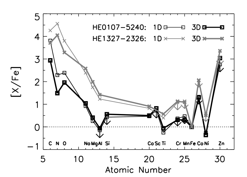
Figure 2: Comparison of 1D LTE (thin lines) and 3D LTE (thick lines) elemental abundance ratios in HE 0107$-$5240 (squares) and HE 1327$-$2326 (crosses); arrows indicate upper limits. The N abundances in HE 0107$-$5240 and HE 1327$-$2326 here shown are both inferred from NH lines. The new solar abundances by Asplund et al. (2005) are used. The adopted 3D$-$1D LTE corrections for the CNO abundances are averages over low-excitation molecular lines.

Table 1: 3D$-$1D LTE corrections applied to the 1D abundances derived for HE 0107$-$5240 and HE 1327$-$2326 from metal lines. Abundances are expressed in the customary logarithmic scale where $\log\epsilon(\mathrm{H})\equiv{12}$. Dots in column 2 indicate that average corrections over two or more lines of the same ion are reported.

			HE 0107$-$5240			HE 1327$-$2326
Ion	$\lambda$ (Å)		$\log\epsilon_{\rm{1D}}$	$\log\epsilon_{\rm{3D}}$		$\log\epsilon_{\rm{1D}}$	$\log\epsilon_{\rm{3D}}$
Li I	$6707.8$		$<1.12$	$<0.94$		$<1.5$	$<1.42$
Na I	…		$1.86$	$1.75$		$3.06$	$3.01$
Mg I	…		$2.41$	$2.33$		$3.63$	$3.63$
Al I	$3961.5$		$<0.93$	$<0.79$		$2.04$	$1.99$
Si I	$3905.5$		$<2.55$	$<2.45$
S  I	$4034.0$		$<7.11$	$<7.15$
Ca I	$4226.7$		$0.99$	$0.84$		$0.95$	$0.85$
Ca II	$3933.7$		$1.44$	$1.24$		$1.52$	$1.37$
Sc II	$3613.8$		$<-1.50$	$<-1.63$
Ti II	…		$-0.62$	$-0.66$		$-0.24$	$-0.31$
Cr I	$4254.3$		$<0.65$	$<0.36$		$<1.09$	$<0.90$
Mn I	$4033.1$		$<0.47$	$<0.08$		$<0.87$	$<0.58$
Fe I	…		$2.06$	$1.83$		$1.79$	$1.55$
Fe II	$5018.4$		$<3.00$	$<3.06$		$<3.01$	$<3.07$
Co I	$3453.5$		$<0.86$	$<0.60$		$<1.34$	$<1.07$
Ni I	$3414.8$		$0.58$	$0.27$		$<1.16$	$<0.86$
Ni I	…		$0.60$	$0.27$
Zn I	$4810.5$		$<1.97$	$<2.02$		$<2.02$	$<2.06$
Sr II	$4077.7$		$<-2.83$	$<-3.00$		$<-1.77$	$<-1.88$
Ba II	$4934.1$		$<-2.33$	$<-2.59$		$<-2.06$	$<-2.25$
Eu II	$4129.7$		$<-1.99$	$<-2.52$

Table 2: Differential 3D and 1D C, N, and O abundances for HE 0107$-$5240 and HE 1327$-$2326 from the analysis of fictitious molecular lines (see section 2.2). The 1D abundances are adopted from the literature, while the 3D abundances are the ones that reproduce the equivalent widths of the fictitious lines calculated with 1D models.

				HE 0107$-$5240			HE 1327$-$2326
Species	$\lambda$ (Å)	$\chi$ (eV)		$\log\epsilon_{\rm{1D}}$	$\log\epsilon_{\rm{3D}}$		$\log\epsilon_{\rm{1D}}$	$\log\epsilon_{\rm{3D}}$
C (CH)	$4360$	0.0		$6.81$	$5.72$		$6.77$	$5.96$
		0.2		$\ldots$	$5.79$		$\ldots$	$6.03$
		0.3		$\ldots$	$5.82$		$\ldots$	$6.07$
		0.5		$\ldots$	$5.90$		$\ldots$	$6.13$
C (C2)	$5160$	0.0		$7.11$	$5.63$
		0.2		$\ldots$	$5.72$
		0.3		$\ldots$	$5.76$
		0.5		$\ldots$	$5.86$
N (CN)	$3880$	0.0		$5.22$ ($4.93$)	$2.91$
		0.2		$\ldots$	$3.04$
		0.3		$\ldots$	$3.12$
		0.5		$\ldots$	$3.27$
N (NH)	$3360$	0.0		$4.83$	$3.78$		$6.58$	$5.76$
		0.2		$\ldots$	$3.85$		$\ldots$	$5.83$
		0.4		$\ldots$	$3.92$		$\ldots$	$5.90$
		0.8		$\ldots$	$4.04$		$\ldots$	$6.01$
O (OH)	$3150$	0.0		$5.66$	$4.95$		$6.65$	$5.80$
		0.5		$\ldots$	$5.04$		$\ldots$	$5.95$
		0.8		$\ldots$	$5.08$		$\ldots$	$6.02$
		1.0		$\ldots$	$5.12$		$\ldots$	$6.07$
		1.5		$\ldots$	$5.19$		$\ldots$	$6.20$

References

- Aoki et al. (2006) Aoki, W., et al. 2006, ApJ, 639, 897
- Asplund et al. (1997) Asplund, M., Gustafsson, B., Kiselman, D., & Eriksson, K. 1997, A&A, 318, 521
- Asplund et. al (1999) Asplund, M., Nordlund, Å., Trampedach, R., & Stein, R. F. 1999, A&A, 346, L17
- Asplund & García Pérez (2001) Asplund, M., & García Pérez, A. E. 2001, A&A, 372, 601
- Asplund (2005) Asplund, M. 2005, ARA&A, 43, 481
- Asplund et al. (2005) Asplund, M., Grevesse, N., & Sauval, A. J. 2005, in ASP Conf. Ser., Cosmic Abundances as Records of Stellar Evolution and Nucleosynthesis, eds. T. G. Barnes III & F. N. Bash (San Francisco: ASP), 25
- Bessell et al. (2004) Bessell, M. S., Christlieb, N., & Gustafsson, B. 2004, ApJ, 612, L61
- Bessell & Christlieb (2005) Bessell, M. S., & Christlieb, N., 2005, IAU Symp. 228, From Lithium to Uranium: Elemental Tracers of Early Cosmic Evolution, eds. V. Hill, P. François, & F. Primas, (Cambridge: CUP), 237
- Christlieb et al. (2002) Christlieb, N., et al. 2002, Nature, 419, 904
- Christlieb et al. (2004) Christlieb, N., Gustafsson, B., Korn, A. J., Barklem, P. S., Beers, T. C., Bessell, M. S., Karlsson, T., & Mizuno-Wiedner, M. 2004, ApJ, 603, 708
- Collet et al. (2005) Collet, R., Asplund, M., & Thévenin, F., 2005, A&A, 442, 643
- Drawin (1968) Drawin, H. W., 1968, Z. Phys., 211, 404
- Drawin (1969) Drawin, H. W. 1969, Z. Phys., 225, 483
- Frebel et al. (2005) Frebel, A., et al. 2005, Nature, 434, 871
- Frebel et al. (2006) Frebel, A., Christlieb, N., Norris, J. E., Aoki, W., & Asplund, M. 2006, ApJ, 638, L17
- Grevesse & Sauval (1998) Grevesse, N., & Sauval, A. J. 1998, Space Sci. Rev., 85, 161
- Gustafsson et al. (1975) Gustafsson, B., Bell, R. A., Eriksson, K., & Nordlund, Å. 1975, A&A, 42, 407
- Karlsson (2006) Karlsson, T. 2006, ApJ, in press (astro-ph/0602597)
- Kurucz (1992) Kurucz, R. L. 1992, Rev. Mexicana Astron. Astrofis., 23, 181
- Kurucz (1993) Kurucz, R. L. 1993, CD-ROM
- Iwamoto et al. (2005) Iwamoto, N., Umeda, H., Tominaga, N., Nomoto, K., & Maeda, K. 2005, Science, 309, 451
- Limongi et al. (2003) Limongi, M., Chieffi, A., & Bonifacio, P. 2003, ApJ, 594, L123
- Meynet et al. (2006) Meynet, G., Ekström, S., & Maeder, A. 2006, A&A, 447, 623
- Meynet & Maeder (2002) Meynet, G., & Maeder, A. 2002, A&A, 390, 561
- Mihalas et al. (1988) Mihalas, D., Däppen, W., & Hummer, D. G. 1988, ApJ, 331, 815
- Nordlund (1982) Nordlund, Å. 1982, A&A, 107, 1
- Picardi et al. (2004) Picardi, I., Chieffi, A., Limongi, M., Pisanti, O., Miele, G., Mangano, G., & Imbriani, G. 2004, ApJ, 609, 1035
- Shigeyama et al. (2003) Shigeyama, T., Tsujimoto, T., & Yoshii, Y. 2003, ApJ, 586, L57
- Spite et al. (2005) Spite, M., et al. 2005, A&A, 430, 655
- Stein & Nordlund (1998) Stein, R. F., & Nordlund, Å. 1998, ApJ, 499, 914
- Suda et al. (2004) Suda, T., Aikawa, M., Machida, M. N., Fujimoto, M. Y., & Iben, I. J. 2004, ApJ, 611, 476
- Umeda & Nomoto (2003) Umeda, H., & Nomoto, K. 2003, Nature, 422, 871
- Weiss et al. (2004) Weiss, A., Schlattl, H., Salaris, M., & Cassisi, S. 2004, A&A, 422, 217