On Iron Enrichment, Star Formation, and Type Ia Supernovae in Galaxy Clusters

Abstract

The nature of star formation and Type Ia supernovae (SNIa) in galaxies in the field and in rich galaxy clusters are contrasted by juxtaposing the build-up of heavy metals in the universe inferred from observed star formation and supernovae rate histories with data on the evolution of Fe abundances in the intracluster medium (ICM). Models for the chemical evolution of Fe in these environments are constructed, subject to observational constraints, for this purpose. While models with a mean delay for SNIa of 3 Gyr and standard initial mass function (IMF) are consistent with observations in the field, cluster Fe enrichment immediately tracks a rapid, top-heavy phase of star formation – although transport of Fe into the ICM may be more prolonged and star formation likely continues to redshifts $<1$. The source of this prompt enrichment is Type II supernovae (SNII) yielding $\geq 0.1~{}{\rm M}_{\odot}$ per explosion (if the SNIa rate normalization is scaled down from its value in the field according to the relative number of candidate progenitor stars in the $3-8~{}{\rm M}_{\odot}$ range) and/or SNIa explosions with short delay times associated with the rapid star formation mode. Star formation is $>3$ times more efficient in rich clusters than in the field, mitigating the overcooling problem in numerical cluster simulations. Both the fraction of baryons cycled through stars, and the fraction of the total present-day stellar mass in the form of stellar remnants, are substantially greater in clusters than in the field.

1 Introduction

Rich clusters of galaxies provide a uniquely amenable setting for the study of the complex processes and consequences of galaxy formation and evolution. As the largest ($\gtrsim 3\ 10^{14}~{}{\rm M}_{\odot}$) virialized objects in the universe, with the deepest potential wells, they retain all of their processed and unprocessed baryonic matter in the form of stars and (predominantly) $\sim 3-10$ keV plasma that are readily studied at infrared/optical/ultraviolet and X-ray wavelengths, respectively.

Rich clusters are sufficiently vast to be considered representative volumes of the universe and are often assumed to be composed of dark matter, stars, and gas in cosmic proportions. However, because clusters originate as extreme peaks in the random field of initial cosmological density fluctuations, the evolution of their constituent galaxies – and by extension the intergalactic medium that they are coupled to – may proceed in a manner that is distinct from their counterparts in the field. The resulting biases must be understood, and taken into account, when generalizing from cluster-based observables in order to draw conclusions about the universe as a whole. In fact, the morphological mix, luminosity function, and star formation history of cluster galaxies all display signatures of the effects of the exceptionally dense environments where they form and develop (Kuntschner et al., 2002; Croton et al., 2005; Schindler et al., 2005; Romeo, Portinari, & Sommer-Larsen, 2005). Since galactic outflows associated with the galaxy formation process, in turn, feed back on the cluster environment by injecting energy and metals into intergalactic plasma, evidence of the cluster/field dichotomy is implanted in the intracluster medium (ICM).

The distinctions between the evolution of baryons in clusters and in the field may be quantified by the juxtaposition of the build-up of heavy metals in the universe inferred from the evolving star formation and supernovae rates with the enrichment history of the ICM in rich galaxy clusters – the dominant reservoir for metals produced by stars in the ensemble of cluster galaxies. Because, under intracluster plasma conditions, abundances of Fe are more easily measured than those of other elements they are derived to redshifts $>1$ and provide the strongest current constraints on the evolution of ICM enrichment.

Mushotzky & Loewenstein (1997) made an initial investigation along these lines based on their analysis of ASCA spectra of clusters out to $z=0.3$, and concluded that ICM enrichment was inconsistent with concurrent estimates of the star formation rate history derived for field galaxies (see, also, Madau, Pozzetti, & Dickinson 1998; Lin & Mohr 2004; Calura & Matteucci 2004). Re-examination of this issue is timely given the extension to higher redshift of ICM Fe abundance measurements made possible with XMM-Newton (Tozzi et al., 2003; Hashimoto et al., 2004; Maughan et al., 2004), and direct estimates of the evolution of supernova rates to comparable redshift in the field (Strolger et al., 2004; Dahlen et al., 2004; Barris & Tonry, 2006) and in clusters (Gal-Yam, Maoz, & Sharon, 2002) that constrain the level of supernova metal production per unit star formation.

Star formation with a standard initial mass function (IMF) produces approximately one core collapse supernova (hereafter, SNII) per hundred solar masses of stars formed, while recent empirical estimates for the specific rate of Type Ia supernovae (SNIa) are an order of magnitude lower. For typical adopted Fe yields of $0.07~{}{\rm M}_{\odot}$ for SNII (slightly higher than the empirical estimate of Elmhamdi, Chugai, & Danziger 2003) and $0.7~{}{\rm M}_{\odot}$ for SNIa (Iwamoto et al., 1999), the estimated universal fraction of baryons in stars of $\sim 0.06$ (Fukugita & Peebles, 2004) thus implies an Fe enrichment per baryon of $\sim 0.065/(1-R)$ relative to solar (solar Fe mass fraction $=0.0013$) that originates in comparable portions from the two classes of supernovae, where $R$ is the stellar mass loss fraction integrated over the age of the universe. Since $R\sim 40$% for a standard IMF (see below), one expects a mean universal Fe enrichment per baryon to about one-tenth solar. While this may be consistent with the low-redshift (non-cluster) IGM (Prochaska 2004; also, see §4.1 below), it falls short by a factor of $\sim 4$ in the ICM (see, also, Pagel 2002). A simple way to account for this shortfall is to invoke a top-heavy IMF (David, Forman, & Jones, 1991; Arnaud et al., 1992; Elbaz, Arnaud, & Vangioni-Flam, 1995; Matteucci & Gibson, 1995; Loewenstein & Mushotzky, 1996; Gibson & Matteucci, 1997) to enhance the formation efficiency of SNII, and perhaps SNIa. Additional variations (some linked to the IMF) include the following: (1) a higher average star formation rate (more SNII and SNIa), (2) a higher incidence of SNIa per star formed, (3) a higher average Fe yield per (Type Ia and/or Type II) supernova, (4) a significant enrichment by a pregalactic stellar population (e.g., Loewenstein 2001). The relative dearth of supernovae in clusters out to the highest redshifts for which the rate is presently constrained highlights the cluster abundance paradox, and begs the question of whether one or more of the standard assumptions (e.g., an IMF that is universal and invariant over time) break down in the universe in general.

This paper aims to evaluate the plausibility and consequences of possible explanations for ICM Fe enrichment, taking into account constraints based on the characteristics of stellar populations in cluster galaxies as well as the observed mean evolution of the cluster SNIa rate and Fe abundance; and, to examine the resulting implications for our understanding of the star formation history (SFH) in the universe and its dependence on environment.

New data on the histories of star formation, supernovae rates, and elemental abundances motivate an approach that goes beyond consideration of the baryon and metal inventories to explicitly model their self-consistent evolution. The framework adopted here for constructing such models, as presented in §2, is kept simple to restrict the number of possible parameters while allowing for consideration of an extensive range in each parameter, and to maintain the transparency of the effects and implications of various assumptions and scenarios. Boundary conditions, source functions, and parameters are initially designed as appropriate for the universe as a whole; but; clear paths for adaptations that might be required for rich galaxy clusters are provided. Models for the chemical evolution of Fe in the ICM are presented in §3, and the requirements on the nature of star formation and supernovae in cluster galaxies imposed by observations are indicated and summarized. §4 includes discussion of the distinction between clusters and the field with respect to their intergalactic media and galaxy populations, and more detailed analysis of galactic outflows and Fe enrichment in clusters. Implications for the nature of SNIa and its environmental dependence, comparisons with results of similar investigations, and possible directions for future model enhancements are also presented in this section. Conclusions, with an emphasis on the dichotomy between clusters and the field, are summarized in §5. I adopt a topologically flat cosmology with Hubble constant $H_{o}=70$ km s^-1, and total and baryonic matter densities, relative to critical, $\Omega_{m}=0.3$ and $\Omega_{b}=0.045$, respectively (e.g., Fukugita & Peebles 2004).

2 Cosmic Chemical Evolution

2.1 Basic Equations

I consider the coupled evolution of the globally averaged densities and metal abundances of the three following baryonic categories: (1) stars that includes main sequence and evolved stars, substellar objects, and stellar remnants; (2) interstellar gas (ISM) defined as the fraction of total matter in the gas phase where stars may form at any time in the history of the universe (regardless of location); and, (3) intergalactic gas (IGM) defined as the remaining, inert (e.g., non-star-forming) fraction of gas-phase matter. Stars and ISM are coupled via star formation and mass return, the ISM and IGM via galactic winds (and, potentially, galactic infall – not explicitly considered here). Type Ia and core collapse supernovae directly enrich the ISM. The evolution equations (Tinsley, 1980; Matteucci & Gibson, 1995; Thomas, Greggio, & Bender, 1998) in rest-frame time for the comoving densities of the three cosmic constituents – $\rho_{\rm stars}$, $\rho_{\rm ISM}$, $\rho_{\rm IGM}$ – and for the mass fractions of their “ith” element – ${f^{i}}_{\rm stars}$, ${f^{i}}_{\rm ISM}$, ${f^{i}}_{\rm IGM}$ – are as follows:

$${{d\rho_{\rm stars}}\over{dt}}=\dot{\rho}_{\rm SF}-\dot{\rho}_{\rm MR},$$ (1)

$${{d\rho_{\rm ISM}}\over{dt}}=-\dot{\rho}_{\rm SF}+\dot{\rho}_{\rm MR}-\dot{\rho}_{\rm GW},$$ (2)

$${{d\rho_{\rm IGM}}\over{dt}}=\dot{\rho}_{\rm GW},$$ (3)

$${{d{f^{i}}_{\rm stars}}\over{dt}}={{\dot{\rho}_{\rm SF}}\over{\rho_{\rm stars}}}({f^{i}}_{\rm ISM}-{f^{i}}_{\rm stars}),$$ (4)

$${{d{f^{i}}_{\rm ISM}}\over{dt}}={{\dot{\rho}_{\rm MR}}\over{\rho_{\rm ISM}}}({f^{i}}_{\rm stars}-{f^{i}}_{\rm ISM})+{{\dot{\rho^{i}}_{\rm SNIa}}\over{\rho_{\rm ISM}}}+{{\dot{\rho^{i}}_{\rm SNII}}\over{\rho_{\rm ISM}}},$$ (5)

and

$${{d{f^{i}}_{\rm IGM}}\over{dt}}={{\dot{\rho}_{\rm GW}}\over{\rho_{\rm IGM}}}({f^{i}}_{\rm ISM}-{f^{i}}_{\rm IGM}),$$ (6)

where the source terms ${\dot{\rho}_{\rm SF}}$, ${\dot{\rho}_{\rm MR}}$, and ${\dot{\rho}_{\rm GW}}$ are the comoving global mass density rates of star formation, mass return, and galactic wind mass transfer from the ISM to the IGM, respectively; and, $\dot{\rho^{i}}_{\rm SNIa}$ and $\dot{\rho^{i}}_{\rm SNII}$ are the density injection rates into the ISM of element “i” from Type Ia and core collapse (mostly Type II) supernovae, respectively. Since the universe is a “closed box,” there are five independent variables; $\rho_{\rm stars}+\rho_{\rm ISM}+\rho_{\rm IGM}=\Omega_{b}\rho_{\rm crit}$, where $\rho_{\rm crit}\equiv 3H_{o}^{2}/8\pi{\rm G}$ is the present-day critical density. Also, the total average baryonic abundance is

$${f^{i}}_{\rm bar}={{\rho_{\rm stars}{f^{i}}_{\rm stars}+\rho_{\rm ISM}{f^{i}}_{\rm ISM}+\rho_{\rm IGM}{f^{i}}_{\rm IGM}}\over{\Omega_{b}\rho_{\rm crit}}}.$$ (7)

2.2 Functions and Parameters

The goal of this paper is to explore the chemical evolutionary implications of the increasingly complete and detailed inventory of matter, and inferred star formation and metal production rates, in the universe; and, to evaluate their applicability to the environment of rich galaxy clusters. As such, empirical quantities and constraints are directly applied to the fullest possible extent, and pegged as points of departure in modeling ICM enrichment.

2.2.1 The Stellar Initial Mass Function

The initial mass function of forming stars (IMF) $\phi(m)\equiv dN/dm$ must be specified to determine the normalization of the observed star formation rate and total stellar mass, the stellar mass fraction recycled to the ISM via mass loss from evolved stars, and the number of supernova explosions per unit mass of star formation. Following Kroupa (2001), I adopt a four-part monotonically decreasing piecewise power-law IMF, extending from $m_{l}=0.01~{}{\rm M}_{\odot}$ in the substellar regime to $m_{u}=150~{}{\rm M}_{\odot}$ (Weidner & Kroupa, 2004; Figer, 2005), with slope ($-dlogN/dlogm$) $\alpha_{0}=0.3$ below the hydrogen-burning mass threshold $m_{H}=0.08~{}{\rm M}_{\odot}$, slope $\alpha_{1}=1.3$ between $m_{H}$ and $m_{B}=0.5~{}{\rm M}_{\odot}$, and slopes $\alpha_{2}$ between $m_{B}$ and $m_{D}$ and $\alpha_{3}$ above $m_{D}$. $\alpha_{2}=\alpha_{3}=2.3$ is adopted as a standard; alternatives are assumed to have a single-slope above $m_{B}$ ($\alpha_{2}=\alpha_{3}$), or an additional break at $m_{D}\geq 2m_{B}$ where the slope changes from $\alpha_{2}=2.3$ to $\alpha_{3}$.

2.2.2 Mass Return

The mass density rate of material recycled from stars to the ISM is

$${\dot{\rho}_{\rm MR}}(t)={\int_{m_{to}}}^{m_{u}}dm\phi(m)\Delta m(m)\dot{n_{\rm SF}}(t-t_{\rm ms}(m)).$$ (8)

The turn-off mass $m_{to}$ is implicitly given by $t_{\rm ms}(m_{to})=\Delta t$ where $t_{\rm ms}(m)$ is the main sequence lifetime of a star of mass $m$ (Schaller et al., 1992) and $\Delta t$ is time since the onset of star formation. $\Delta m(m)$ is the mass returned by stars of main sequence mass $m$, and is assumed independent of time. The star formation rate density $\dot{n_{\rm SF}}\equiv{\dot{\rho}_{\rm SF}}/{{\int_{m_{l}}}^{m_{u}}}dm\phi(m)m$.

$\Delta m(m)$ is derived using appropriate remnant masses, $m_{\rm rem}$, in the white dwarf, neutron star, and black hole regimes (Prantzos, Casse, & Vangioni-Flam, 1993; van den Hoek & Groenewegen, 1997; Fryer & Kalogera, 2001; Woosley, Heger, & Weaver, 2002) as follows:

$$\Delta m(m)=m-m_{\rm rem}(m);$$ (9)

$$m_{\rm rem}=0.45+0.119m,\ m\leq 8;$$ (10)

$$m_{\rm rem}=1.4,\ 8\leq m\leq 21;$$ (11)

$$m_{\rm rem}=1.4+0.717(m-21),\ 21\leq m\leq 33;$$ (12)

$$m_{\rm rem}=10,m\geq 33,$$ (13)

where $m$ is in ${\rm M}_{\odot}$.

The integrated fraction of mass formed into stars that is returned to the ISM up to the present epoch ($t_{\rm now}=13.47$ Gyr) is

$$R={{{{\int_{m_{to}(t_{\rm now})}}^{m_{u}}}dm\phi(m)\Delta m(m)}\over{{\int_{m_{l}}}^{m_{u}}dm\phi(m)m}},$$ (14)

where $m_{to}(t_{\rm now})\sim 0.9~{}{\rm M}_{\odot}$ is the present epoch main sequence turn-off mass. Under the instantaneous recycling approximation (IRA: $t_{\rm ms}(m)\rightarrow 0$ for all $m$), ${\dot{\rho}_{\rm MR}}(t)=R{\dot{\rho}_{\rm SF}}$. The exact treatment (equation 8) is adopted for calculating $\dot{\rho}_{\rm MR}$, since star-formation histories that decline on short timescales are considered. However, in deriving equations 4 and 5, the rate of metal transfer to the ISM via stellar mass loss at time $t$ is estimated as $\dot{\rho}_{\rm MR}(t){f^{i}}_{\rm stars}(t)$ (rather than by evaluating an integral similar to that in equation 8).

2.2.3 Star Formation

Estimates of ${\dot{\rho}_{\rm SF}}$, corrected for dust, are compiled and compared in Hopkins (2004), and fitted to analytic functions in Bell (2005) and Strolger et al. (2004). The star formation rate is renormalized to assure that

$${\int_{t_{\rm form}}}^{t_{\rm now}}dt{\dot{\rho}_{\rm SF}}(t)={{\rho_{\rm stars}({t_{\rm now}})-\rho_{\rm stars}({t_{\rm form}})}\over{(1-R)}},$$ (15)

where $\rho_{\rm stars}({t_{\rm now}})$ is the cosmic density in stars observed today, and $\rho_{\rm stars}({t_{\rm form}})$ the density of zero-metallicity (Population III) “seed” stars predating the time, $t_{\rm form}$, when galaxy formation begins and the integration of the set of equations (1)–(6) is initiated.

2.2.4 Core Collapse Supernovae

The mass density injection rate of element “i” into the ISM by core collapse supernova of massive stars (“SNII”) is

$${{\dot{\rho}_{\rm SNII}}}^{i}(t)={\int_{m_{1}}}^{m_{2}}dm\phi(m){y_{\rm SNII}}^{i}(m)\dot{n_{\rm SF}}(t-t_{\rm ms}(m)),$$ (16)

where $m_{1}<m<m_{2}$ is the range of SNII progenitor masses and ${y_{\rm SNII}}^{i}(m)$ is the nucleosynthetic yield of element “i” from a progenitor of mass $m$. Instantaneous enrichment is an adequate approximation for these short-lived stars, reducing equation (16) to

$${{\dot{\rho}_{\rm SNII}}}^{i}(t)=K_{\rm SNII}{\dot{\rho}_{\rm SF}}(t)\langle{y_{\rm SNII}}^{i}\rangle,$$ (17)

where $K_{\rm SNII}\equiv{{\int_{m_{1}}}^{m_{2}}}dm\phi(m)/{{\int_{m_{l}}}^{m_{u}}}dm\phi(m)m$ is the number of SNII per unit mass of star formation, and $\langle{y_{\rm SNII}}^{i}\rangle\equiv{{\int_{m_{1}}}^{m_{2}}}dm\phi(m){y_{\rm SNII}}^{i}(m)/{{\int_{m_{l}}}^{m_{u}}}dm\phi(m)$ the mean SNII yield of the “ith” element.

2.2.5 Type Ia Supernovae

In light of the multiplicity of theoretical predictions for the SNIa rate (Barris & Tonry 2006, and references therein) I adopt the semi-empirical formalism of Strolger et al. (2004) and Dahlen et al. (2004), determining the mass density injection rate of element “i” by SNIa into the ISM from

$${{\dot{\rho}_{\rm SNIa}}}^{i}(t)=\dot{n_{\rm SNIa}}(t){y_{\rm SNIa}}^{i},$$ (18)

and

$$\dot{n_{\rm SNIa}}(t)=\nu{\int_{t_{\rm form}}}^{t}dt^{\prime}{\dot{\rho}_{\rm SF}}(t^{\prime})\Phi(t-t^{\prime}),$$ (19)

where $\nu$ is the number of SNIa progenitor systems per unit mass of star formation, ${y_{\rm SNIa}}^{i}$ is the SNIa nucleosynthetic yield of element “i” (assumed to be constant), and $\Phi(t_{d})$ is the normalized delay time distribution function (DTDF) parameterized using the Gaussian distribution found by Strolger et al. (2004) and Dahlen et al. (2004) to explain the observed evolution of the SNIa rate,

$$\Phi(t_{d})=(2\pi\sigma^{2})^{-1}e^{-[(t_{d}-t_{c})^{2}/2\sigma^{2}]}.$$ (20)

2.2.6 Star-Formation-Induced Galactic Wind

I assume that supernova explosions drive outflow of material from the ISM to the IGM and that the mass loss rate per unit volume is proportional to the total supernova rate and the ISM density,

$${\dot{\rho}_{\rm GW}}(t)=K_{\rm GW}(\dot{n_{\rm SNIa}}(t)+K_{\rm SNII}{\dot{\rho}_{\rm SF}}(t))\rho_{\rm ISM}.$$ (21)

Metal-rich gas is not preferentially ejected, and SNIa and SNII are assumed to contribute to driving outflows with equal efficiency. Given an observationally determined present-day ISM density, $\rho_{\rm ISM}({t_{\rm now}})$, setting the galactic wind strength, $K_{\rm GW}$ is equivalent to assuming a value for the initial ISM density, $\rho_{\rm ISM}({t_{\rm form}})$. I calculate this relationship by integrating equation (2) from $t_{\rm now}$ to $t_{\rm form}$. In the absence of infall, $\rho_{\rm ISM}({t_{\rm form}})$ must be sufficient to account for all the star formation since $t_{\rm form}$, $\rho_{\rm stars}({t_{\rm now}})-\rho_{\rm stars}({t_{\rm form}})$, and is bounded above by the total baryon density. That is, allowed values of $K_{\rm GW}$ are those that yield

$$\rho_{\rm ISM,min}<\rho_{\rm ISM}({t_{\rm form}})<\rho_{\rm ISM,max},$$ (22)

where $\rho_{\rm ISM,min}=\rho_{\rm ISM}({t_{\rm now}})+(\rho_{\rm stars}({t_{\rm now}})-\rho_{\rm stars}({t_{\rm form}}))$ corresponds to no wind, and $\rho_{\rm ISM,max}=\Omega_{b}\rho_{\rm crit}-\rho_{\rm stars}({t_{\rm form}})$ to a wind with maximum integrated mass outflow (“maximum wind”).

Although ram-pressure stripping may be important in determining the abundance gradient, it is generally thought to account for a small (though significant) fraction of total ICM metal enrichment (e.g., Domainko et al. 2006). However, it may play a role in extending the epoch of mass transfer from galaxies to the ICM. I consider an additional galactic outflow term that may (at least in part) be associated with this mechanism (see §§3.1.1, 4.2).

2.2.7 Boundary Conditions

Equations (1), (2), (4), (5), and (6) are integrated from $t_{\rm form}$ to $t_{\rm now}$, with metal-free initial conditions: ${f^{i}}_{\rm stars}={f^{i}}_{\rm ISM}={f^{i}}_{\rm IGM}=0$. A small seed stellar density is assumed, $\rho_{\rm stars}({t_{\rm form}})=\Omega_{\rm III}\rho_{\rm crit}$; $\rho_{\rm ISM}({t_{\rm form}})$ is a free parameter within the limits of equation (22).

2.2.8 Standard and Varying Parameters and Assumptions

Standard boundary conditions include the formation epoch of the first Population II stars ($t_{\rm form}=4.66\ 10^{8}$ yr, corresponding to redshift 10 for the adopted cosmology), the (Population III) stellar density $\Omega_{\rm III}\rho_{\rm crit}=3\ 10^{-6}\rho_{\rm crit}$ (Ostriker & Gnedin, 1996), and the stellar ($\rho_{\rm stars}({t_{\rm now}})=0.00267\rho_{\rm crit}$) and ISM ($\rho_{\rm ISM}({t_{\rm now}})=0.00078\rho_{\rm crit}$) densities at the present epoch (Fukugita & Peebles, 2004).

The IMF parameters are the slope at high mass, $\alpha_{3}$, and transition mass, $m_{D}$, to this slope from $\alpha_{2}=2.3$. The choice of IMF, in turn, determines the mass return fraction $R$ (equation 14) and renormalization factor for the star formation rate (equation 15), and the number of SNII per unit mass of star formation, $K_{\rm SNII}$. In the standard model, $\alpha_{3}=2.3$, $R=0.393$ (the IRA value is 0.405), and $K_{\rm SNII}=0.0104~{}{\rm M}_{\odot}^{-1}$ for $m_{1}=8~{}{\rm M}_{\odot}$ and $m_{2}=m_{u}=150~{}{\rm M}_{\odot}$. The renormalization factors for the Bell (2005) and Strolger et al. (2004) star formation rate parameterizations are 0.94 and 0.62, respectively. I adopt the Bell (2005) SFH parametrization as standard. Since the Strolger et al. (2004) rate differs most dramatically in shape at low redshift where a relatively small fraction of the integrated star formation occurs, our results are insensitive to this choice (the renormalized functions are compared in Figure 2; see below). Adoption of the standard $K_{\rm SNII}$ and ${\dot{\rho}_{\rm SF}}(t)$ provides consistency with observed SNII rate evolution to redshift 1 (Strolger et al. 2004, Dahlen et al. 2004; see, also, Figure 3 below). There is sufficient theoretical uncertainty in the SNII synthesis of Fe that the IMF-averaged SNII Fe yield, $\langle{y_{\rm SNII}}^{\rm Fe}\rangle$, is simply left as a parameter with standard value $0.07~{}{\rm M}_{\odot}$.

Standard SNIa parameters include mean delay time $t_{c}=3$ Gyr, dispersion $\sigma=0.2t_{c}$, and normalization $\nu=1.5\ 10^{-3}$ SNIa ${{\rm M}_{\odot}}^{-1}$ (see, also, Gal-Yam & Maoz 2004, Greggio 2005) that provide the best fit to the observed SNIa rate evolution for the Bell (2005) star formation rate parametrization (these slightly differ from their values in Dahlen et al. 2004 due to the different adopted star formation rate). I focus on Fe in this paper (thus justifying the neglect of non-explosive production in equation 5); a SNIa Fe yield ${y_{\rm SNIa}}^{\rm Fe}=0.7~{}{\rm M}_{\odot}$ is adopted as standard.

For the above standard parameters and functions, one may vary the galactic wind factor from $K_{\rm GW}=0$ to ${K_{\rm GW}}^{\rm max}$, where $\Omega_{b}\rho_{\rm crit}{K_{\rm GW}}^{\rm max}=3.05\ 10^{3}~{}{{\rm M}_{\odot}}$ is such that all of the IGM originates in the ISM.

2.2.9 A Note on Varying the IMF

The standard model IMF (with slope 2.3 above $0.5~{}{\rm M}_{\odot}$), if assumed universal, provides mutual consistency among observations of the star formation and SNII rates and build-up of stellar mass (Bell, 2005; Drory et al., 2005; Gwyn & Hartwick, 2005), and with the luminosity density of the universe (Baldry & Glazebrook, 2003). If the slope is significantly flatter, (1) the higher stellar mass loss return fraction (Figure 1) implies that a higher star formation rate than is observed would be required to produce the observed amount of stars (Figure 2); and, (2) the implied SNII rate would be greater than observed (Figure 3a). Conversely, a steeper high mass IMF slope (i.e., $\alpha_{2}=2.8$; see Kroupa & Weidner 2003) significantly underpredicts the observed SNII rate (Weidner & Kroupa, 2005) unless the transition at $m_{D}$ is pushed to high mass (Figure 3b).

2.3 Enrichment in the Standard Model

The chemical evolution of Fe in the standard model (see entries “1N2.3” in Tables 1 and 2) provides predictions to be compared with abundance measurements in stars and interstellar gas in field galaxies, and in the intergalactic medium. This serves to indicate possible shortcomings in the model and provide a baseline for evaluating what manner of extension or variation might be required to explain Fe abundances in rich galaxy clusters. Integrated over a Hubble time, the total stellar Fe yield (relative to solar) in the standard model is 1.3 (58/42% from SNIa/SNII) corresponding to an enrichment of 0.13 averaged over all baryons (Table 2). The model-predicted $z=0$ SNII and SNIa rates (Table 2) are consistent with observations (Cappellaro, Evans, & Turatto, 1999).

The distribution of Fe among stellar, ISM, and IGM components as a function of time depends on the strength and time-dependence of galactic outflow. The more numerous SNII dominate the galactic wind term (equation 21), but SNIa contribute the majority of Fe enrichment – and do so with a significant lag with respect to the accumulation of stellar mass and the ejection of SNII-enriched material into the IGM. This results in a relatively recent ($z<1$) build-up of Fe in the stars (Figure 4a) and ISM (Figure 4b) and a substantial Fe mass fraction contained in these components at the present epoch. As a result, little more than half of the total Fe production is injected into the IGM for a “maximum” wind (Figure 5). A reapportionment that boosts the IGM Fe fraction requires extending the outflow duration, a possible mechanism considered in detail below.

A comparison, focusing on the $z>2$ universe, of the enrichment buildup in these models with the inventory of metals derived from observations of damped Ly$\alpha$ systems, the Ly$\alpha$ forest, and Lyman break galaxies is made in §4.1 below.

3 Modeling Fe Enrichment of the Intracluster Medium

The formalism of the previous section can be directly adapted to investigate the chemical evolution of stars, ISM, and IGM (ICM) in clusters – assuming that they are closed boxes – by simply rescaling the physical densities by the mean cluster baryon overdensity factor (i.e., the total overdensity multiplied by a cluster baryon “bias” factor – see, e.g., Allen et al. 2004), $\delta\sim 10^{2}$. Clearly, the standard model must be adjusted in application to clusters as it predicts an IGM Fe abundance $>5$ times smaller than measured in the ICM.

There is strong evidence that star formation ensued more quickly in clusters with respect to the field, as one might expect in regions of highest initial overdensity (Schindler et al., 2005; Romeo, Portinari, & Sommer-Larsen, 2005). However, this in itself does not result in enhanced enrichment if the integrated star formation and IMF are unaltered. Estimates for the rich cluster mass fraction in stars vary, but are typically twice the estimated universal value of $\sim 0.06$ (see §4.4). Nevertheless, the Fe enrichment shortfall persists if the yield per star formed is that of the standard model (Pagel, 2002; Nagashima et al., 2005a). Moreover, there are claims of still higher stellar mass fractions in galaxy groups (Parker et al., 2006; Eke et al., 2005); yet, group IGM Fe abundances are not generally higher than in the ICM (though groups may not be closed boxes). Therefore, as elaborated on below, a top-heavy IMF may be required to explain the observed 0.4 solar ICM Fe abundance.

While much of the star formation in intermediate and low mass galaxies occurs after the peak in the universal SFH at $z\approx 1$, the most massive (elliptical) galaxies were assembled and their star formation completed at earlier epochs (Saracco et al., 2004; Bell, 2005; Fontana et al., 2004; McCarthy et al., 2004; Hammer et al., 2005; Thomas et al., 2005; Caputi et al., 2005; Jimenez et al., 2005; Papovich et al., 2006). Since the fraction of stars formed in elliptical galaxies is higher in clusters and star formation is expected to be accelerated in denser environments (Kodama et al., 2004; Thomas et al., 2005), I consider an enhancement in star formation, referred to as the “rapid mode”, with an exponential time-dependence, $\dot{\rho}_{\rm XSF}\propto e^{-t/(\tau_{X}t_{\rm now})}$. These stars may reside in protogalactic fragments, or even in isolation in intracluster space (Lin & Mohr, 2004; Zaritsky, Gonzalez, & Zabludoff, 2004). Star formation in these extended models is characterized by the dimensionless parameter $\tau_{X}$, the normalizations of the “normal” (i.e., with the same time-dependence as the average field star formation rate; see Figure 2) and rapid star formation modes (expressed, in Table 1, as the present-epoch stellar baryon fractions: $f_{\rm stars}$ and $f_{\rm Xstars}$, respectively), and the IMF of each mode (i.e., $m_{D}$, $\alpha_{3}$, $m_{DX}$, $\alpha_{3X}$; in practice, when considering a nonzero exponential star formation contribution, $\alpha_{3}=2.3$ is often adopted). For the models discussed in the next section $\tau_{X}=0.1$ is chosen.

3.1 Accounting for Fe, and its Evolution, in Clusters

3.1.1 General Considerations

If the ratio of intergalactic gas to stars in clusters is the same as the universal average, $\sim 16$, severe difficulties, as described in §2, emerge in constructing models that reproduce observed cluster Fe abundances. This is illustrated in Figure 6, where the solid curve plots the relationship between the ratio of the Fe abundance in galaxies (i.e., a mass-weighted average of stars and ISM) to that in the ICM versus the mass fraction of Fe in the ICM, assuming the universal IGM fraction of 0.924. A conservative upper limit to the ratio of galactic-to-intergalactic Fe abundances of 5 requires that $>70$% of the Fe reside in the ICM. However, as indicated above for the standard model, if galactic winds are driven by star formation while enrichment is more prolonged due to the delay in SNIa explosions, then more than half of the Fe is locked up in galactic stars. This results in a galaxy/ICM Fe abundance ratio $>12$ (Figure 6). This problem is exacerbated if (as expected) star formation is accelerated in clusters relative to the field, but is mollified if star formation is more efficient. A galactic-to-intergalactic Fe abundance ratio of 5 implies an ICM Fe mass fraction $\sim 55$% ($\sim 45$%) for a stellar mass fraction that is twice (three times) the universal average (see dotted and dashed curves if Figure 6).

To transport sufficient Fe from galaxies to the ICM requires an outflow that is extended in time if the standard treatment of SNIa rates and yields, as previously defined, is adopted. I thus modify equation (21) by adding one of the two following terms: (1) ${\dot{\rho}_{\rm GW}}(t)\rightarrow{\dot{\rho}_{\rm GW}}(t)+\rho_{\rm ISM}/t_{\rm wind}$ (additional exponential outflow term), or (2) ${\dot{\rho}_{\rm GW}}(t)\rightarrow{\dot{\rho}_{\rm GW}}(t)+\rho_{\rm ISM,min}/\Delta t_{\rm wind}$ (additional constant outflow term), where $\rho_{\rm ISM,min}$ is defined following equation (22) and $t_{\rm wind}$ and $\Delta t_{\rm wind}$ are additional parameters (that modify the relationship between $K_{\rm GW}$ and $\rho_{\rm ISM}({t_{\rm form}})$).

3.1.2 Results of Representative Models

The equations of §2 are solved for an extensive multi-dimensional grid of SFHs ($f_{\rm stars}$, $m_{D}$, $\alpha_{3}$, $f_{\rm Xstars}$, $m_{DX}$, $\alpha_{3X}$) and outflow ($t_{\rm wind}$ or $\Delta t_{\rm wind}$, $K_{\rm GW}$ or – equivalently – $\rho_{\rm ISM}({t_{\rm form}})$) parameters. Conservatively, further consideration is restricted to models that produce ICM Fe mass fractions of $40-80$%. Integrated supernovae Fe yields per baryon of $\sim 0.5-1$ relative to solar are thus implied, given the 0.4 solar ICM Fe abundance. The outflow strength and evolution must be adjusted to release sufficient Fe into the ICM from galaxies, and affects how quickly the high ICM Fe abundance accumulates.

Of course, there is a large parameter degeneracy among models that predict 0.4 solar ICM Fe abundance at $z=0$. These are constructed and evaluated in the context of recent data on cluster Fe abundance and SNIa rate evolution, not necessarily to narrowly determine these parameters, but to reveal the general distinctions between these models and those constructed to explain standard universal chemical evolution. We will see that none of the models are fully satisfactory, thus motivating exploration of additional variations.

Details of an illustrative cross section of models that are examined in more detail are displayed in Table 1. These are labeled by (1) the present-day total stellar mass fraction relative to the universal value (there are equal contributions from normal and rapid modes in all hybrid SFH models), and (2) whether the SFH follows the normal (N) or rapid (R) mode functional form, or a hybrid (H) of the two. They are further denoted by (3) the high mass IMF slope ($\alpha_{3}$ or $\alpha_{3X}$), where the rapid mode slope is used for the hybrid SFH models (except for model 1H0.8Wc where $\alpha_{3}=1.8$, the normal mode slope is 2.3 for all H-models; Table 1). The break mass, $m_{D}$ or $m_{DX}$, is usually $2~{}{\rm M}_{\odot}$ and introduces no additional ambiguity otherwise. Finally (4), the designation “Wx” (“Wc”) denotes whether an extended exponential (constant) outflow term is included, with the normalized timescale displayed in Table 1. The choice of outflow form and timescale, as well as the parameter $\rho_{\rm ISM}({t_{\rm form}})$ (expressed in Table 1 as the initial baryon mass fraction in the ISM, $f_{\rm ISM}({t_{\rm form}}$)), likewise introduce no ambiguities – i.e. an optimal value is selected for each SFH/IMF combination. The models appearing above the demarcation line in Tables 1 and 2 follow the standard SNIa and SNII treatments explained in §2, and have $t_{\rm form}$ corresponding to $z=10$. This subset demonstrates the diversity of predicted model outcomes and level of consistency with cluster data, and how these vary with changes in the input parameters.

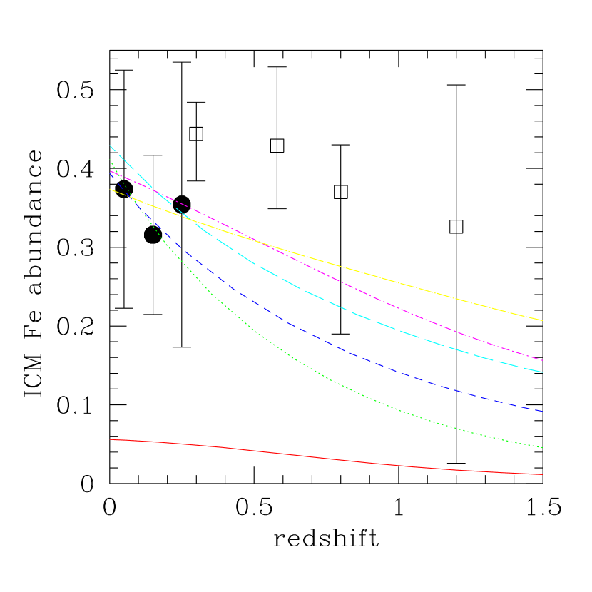
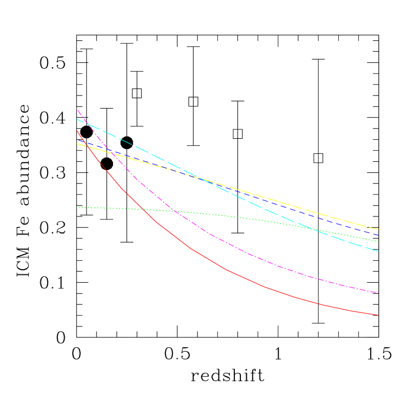
Figure 7: left(a): Evolution of ICM Fe abundance for Models 1N2.3, 1N1.05Wc, 1H0.8Wc, 1R1.05Wc, 2H1.3Wx, and 2R1.55Wx (solid, dot, short-dash, long-dash, dot-short-dash, dot-long-dash line-type respectively). right(b): Evolution of ICM Fe abundance for Models 2H0.8Wc, 2H1.05, 2H1.05Wx, 2H1.3Wx, 2H1.3Wc, and 2H1.55Wx (solid, dot, short-dash, long-dash, dot-short-dash, dot-long-dash line-type, respectively). Filled circles denote abundances derived from ASCA data of $kT>2$ keV clusters from Baumgartner et al. (2005) with 90% confidence uncertainties, open squares those from XMM-Newton data of $kT>5$ keV clusters from Tozzi et al. (2003) with $2\sigma$ uncertainties. See §3 and Tables 1 and 2 for model details.

The present-day characteristics of these models are displayed in Table 2, and the evolution of the ICM Fe abundance back to $z=1.5$ for these models is illustrated and compared to observations in Figures 7ab. Since infall is not considered, ISM abundances are significantly higher than stellar abundances (see Figure 4; also, Figure 8b below; and, Pipino et al. 2005). Since one might expect higher metallicity ISM to form stars more readily and equalize these, I define the “galactic” abundance, ${\langle{\rm Fe}\rangle}_{\rm gal}$, as the mass-weighted average of the ISM and galaxy Fe abundances (see Table 2); ${\langle{\rm Fe}\rangle}_{\rm gal}$ serves as an upper limit to the stellar Fe abundance.

The following general statements can be made. (1) As discussed above, a model with the form of the universal SFH, the universal fraction of baryons in stars, and standard transformation from star formation rate to supernova enrichment, falls many factors short of providing sufficient Fe (e.g., Model 1N2.3; solid curve in Figure 7a). (2) As illustrated by Model 2H1.05 (dotted curve in Figure 7b), basic models where the outflow strictly traces the supernova rate generally predict fractions of Fe locked up in stars (and ISM) that are too high to yield consistency with present-day ICM Fe abundances (for a reasonable galactic abundance, see discussion above). (3) Flattening the IMF whilst retaining the standard model SFH form (e.g., Model 1N1.05Wc; dotted curve in Figure 7a) produces the observed $z=0$ ICM Fe abundance if an extended outflow is assumed; however, the buildup of Fe is too recent to be consistent with X-ray spectroscopy of clusters over redshifts 0–1 (Tozzi et al., 2003; Hashimoto et al., 2004; Maughan et al., 2004). This is also the case in other models with insufficient massive star formation at high redshift, including Model 1H0.8Wc where the universal value for the baryon fraction in stars originates equally in normal and rapid star formation modes (short-dashed curve in Figure 7a).

The observed magnitude and mild evolution of the ICM Fe abundance is fairly well reproduced in a variety of models with a top-heavy IMF, prompt star formation, and extended outflow. These include Models 1R1.05Wc and 2R1.55Wx where all star formation is in rapid mode (long-dashed and dot-long-dashed curves in Figure 7a, respectively), and in a number of hybrid (“2H”) models that include both star formation modes.

The “2H” series of models (see Tables 1 and 2, and Figure 7b) are those characterized by SFHs producing twice the universal average of the present-day baryon fraction in stars (see §4.4), with half originating in normal star formation mode with a standard IMF and half in rapid mode with a steeper high mass IMF, that yield $z=0$ Fe abundances $\sim 0.4$ solar. These provide fairly good explanations of the observed ICM Fe abundances over $z=0-1$, provided that the IMF is sufficiently top heavy and the outflow is of sufficient magnitude and duration (Models 2H1.05Wx, 2H1.3Wx, 2H1.55Wx). Earlier ICM enrichment in models with exponential winds, compared to that in models with constant winds, results in a flatter decline in Fe abundance with redshift and a better match to the observed ICM Fe evolution. The effect of varying the supernova wind strength over the full physically allowed range is illustrated in Figures 8ab; Fe abundances span a full range $\Delta{\langle{\rm Fe}\rangle}_{\rm ICM}\sim 0.1$ at each redshift.

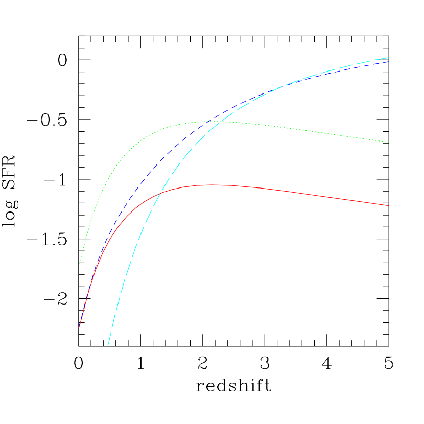
Figure 9: Star formation histories for Models 1N2.3, 1N1.05Wc, 2H1.3Wx, and 2R1.55Wx (solid, dot, short-dash, long-dash line-types, respectively.) Star formation rates are expressed in units of $\delta^{-1}~{}{\rm M}_{\odot}~{}{\rm Mp}c^{-3}~{}{\rm yr}^{-1}$ where $\delta$ is the baryon overdensity. The Model 1N2.3 curve matches the (scaled) observed SFH for field galaxies.

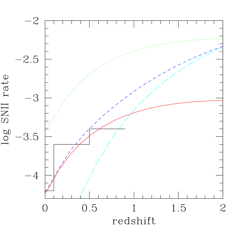
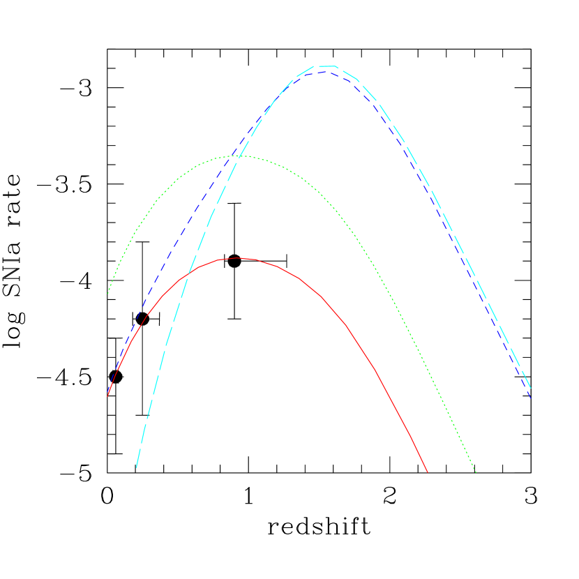
Figure 10: left(a): Same as Figure 9 for SNII rate histories, with the observed field rate histogram reproduced from Figure 3. right(b): Same as (a) for SNIa rate history. Errorbars are observed cluster SNIa rates (with $1\sigma$ errors) from Table 7 of Gal-Yam, Maoz, & Sharon (2002). Supernova rates are in units of $\delta^{-1}~{}{\rm Mp}c^{-3}~{}{\rm yr}^{-1}$. As in Figure 9, solid curves match the (scaled) observed field rates.

The SFHs for Models 1N2.3, 1N1.05Wc, 2H1.3Wx, and 2R1.55Wx are shown in Figure 9 (the latter two are representative of the best fits to the observed Fe abundance evolution from Figures 7ab, the former two are included for comparative purposes). SFHs in dual-mode (hybrid) models follow the (scaled) field SFH out to $z=1$ since a standard IMF is assumed for the normal mode. The star formation rates in the models with a rapid component, of course, greatly exceed the field value at high redshift; their SFHs resemble those inferred in massive galaxies (Heavens et al., 2004; Yee et al., 2005). Similar enhancements are realized in the Type II and Type Ia supernova rates (Figures 10ab), although the SNIa explosion delay leads to a turnover in the rate at high redshift. The solid curves (Model 1N2.3) match the rates in the field, while the errorbars are cluster rates measured by Gal-Yam, Maoz, & Sharon (2002). The latter are converted from units of “SNU” (supernovae per 100 years per $10^{10}$ solar $B$-band luminosities) assuming that clusters have twice the overall stellar mass-to-light ratio and twice the stellar fraction as in the field, and show surprising consistency with the field rate evolution. Large intermediate redshift SNIa rates in clusters are predicted in these models where the abundance and evolution of Fe in the ICM is explained via SNII and SNIa from a top-heavy IMF enhancement in high redshift star formation, and where the SNIa delay-time characteristics and relative normalization are the same as in the field. These rates are marginally inconsistent with the empirical cluster estimates, a characteristic shared by all models of the type discussed up to this point that successfully explain the ICM Fe abundance and its evolution.

Additional models with empirically motivated variations in formation epoch and various supernova input parameters are described below the demarcation line in Tables 1 and 2, and discussed in the following three subsections.

3.1.3 Reducing the Mean Supernovae Delay Time

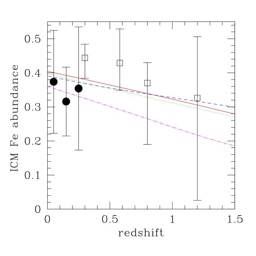
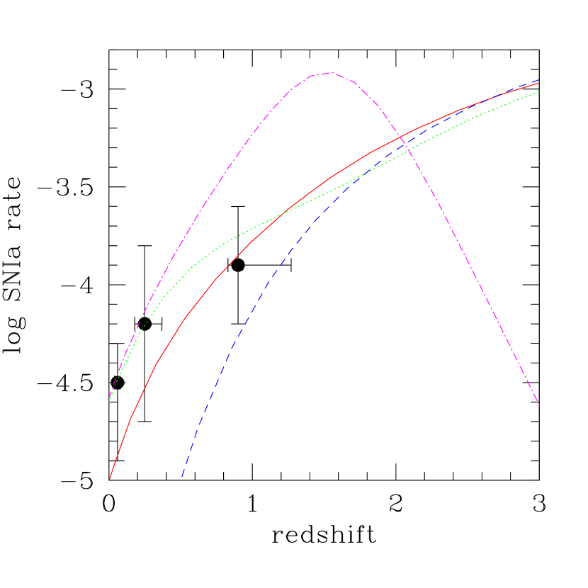
Figure 11: left(a): Evolution of ICM Fe abundance for models with reduced SNIa delay times, 2H1.05WxSt1, 2H1.05WxSt2, 2R1.55WxSt, (solid, dot, short-dash curves respectively). For comparison, the evolution for model 2H1.05Wx from Figure 7a is re-plotted (dot-dashed curve). right(b): Same as (a) for SNIa rate (in $\delta^{-1}~{}{\rm Mp}c^{-3}~{}{\rm yr}^{-1}$) history.

In order to construct models that better agree with the cluster SNIa data, I consider a reduction, from 3 to 0.5 Gyr, in the mean SNIa delay interval (Maoz & Gal-Yam, 2004) that may be applied to all SNIa (Model 2H1.05WxSt1 in Tables 1 and 2). Mannucci, della Valle, & Panagia (2006) argue for a bimodal population of SNIa that includes one subclass that is associated with active star formation and characterized by delay times that are insignificant relative to the duration of the star formation epoch, and another subclass associated with quiescent secular evolution that is characterized by a broad distribution extending to long delay times. I also, therefore, consider models where the reduction in mean delay time is exclusively applied to SNIa originating in rapid star formation mode (Model 2R1.55WxSt – with only rapid mode star formation, Model 2H1.05WxSt2). The results are shown in Table 2 and Figures 11ab. Agreement with observations of the ICM Fe abundance evolution is significantly improved, and the $z<1$ SNIa rate histories – that now more closely trace the SFHs – in the hybrid SFH models are in better accord with the observational constraints.

3.1.4 Reducing the Formation Redshift

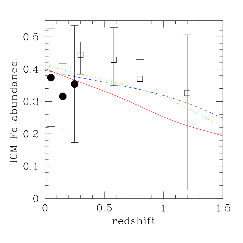
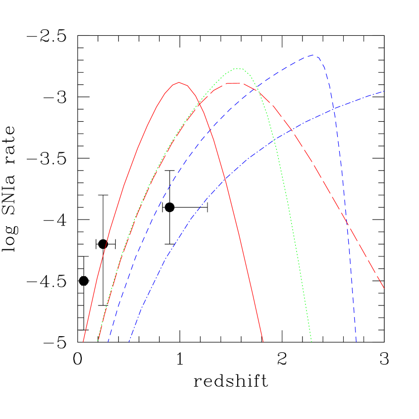
Figure 12: left(a): Evolution of ICM Fe abundance for models with rapid mode star formation initiating at $z=3$, rather than $z=10$. Shown are models with mean SNIa delay times of 3 (2R1.55WxSz; solid curve), 1.5 (2R1.55WxStpz; dotted curve), and 0.5 (2R1.55WxStz; short-dashed curve) Gyr. right(b): Same as (a) for SNIa rate (in $\delta^{-1}~{}{\rm Mp}c^{-3}~{}{\rm yr}^{-1}$). The $z=10$ counterparts for delay times of 3 (2R1.55Wx; long-dashed curve) and 0.5 (2R1.55WxSt; dot-dash curve), Gyr are reproduced.

Since the heretofore considered rapid star formation models appear to underpredict the present-day cluster SNIa rate, I consider a sequence of rapid SFH models where the initiation of star formation is moved forward from $z(t_{\rm form})=10$ to $z(t_{\rm form})=3$. The outcomes of three such models (2R1.55WxSz, 2R1.55WxStpz, 2R1.55WxStz; Table 1), distinguished by mean SNIa delay times ($t_{cX}$) that are, respectively, 3, 1.5, and 0.5 Gyr are summarized in Table 2 and Figures 12ab. The SNIa rate evolution in these models, optimized to match the observed cluster Fe abundance evolution (Figure 12a,) is compared to that in models with earlier formation epoch in Figure 12b. Delaying the onset of star formation improves the match to cluster SNIa rate observations for $t_{cX}=0.5$ Gyr, but worsens it for $t_{cX}=3$ Gyr.

3.1.5 Naturally Reducing the SNIa Rate

I also construct models with “naturally” reduced rapid star formation mode specific SNIa rate – i.e. the scaling is calculated assuming that a universal fraction of $3-8~{}{\rm M}_{\odot}$ stars forms SNIa progenitor binaries. I consider models characterized by $m_{DX}=m_{D}=2~{}{\rm M}_{\odot}$, $\alpha_{3}=2.3$, $t_{c}=3$ Gyr, $z(t_{\rm form})=10$ or 3, $t_{cX}=3$ or 0.5 Gyr, and $\langle{y_{\rm SNII}}^{\rm Fe}\rangle=0.07$ or $0.10~{}{\rm M}_{\odot}$; and, focus here on an illustrative subset of “2H” and “2R” models (i.e., where 12% of present-day cluster baryons are in stars formed either in equal proportions in normal and rapid mode, or exclusively in rapid mode) with $\alpha_{3X}=1.05$ and 1.55, respectively. The corresponding rapid mode SNIa rate reduction factors are 0.26 and 0.66.

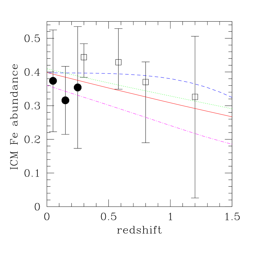
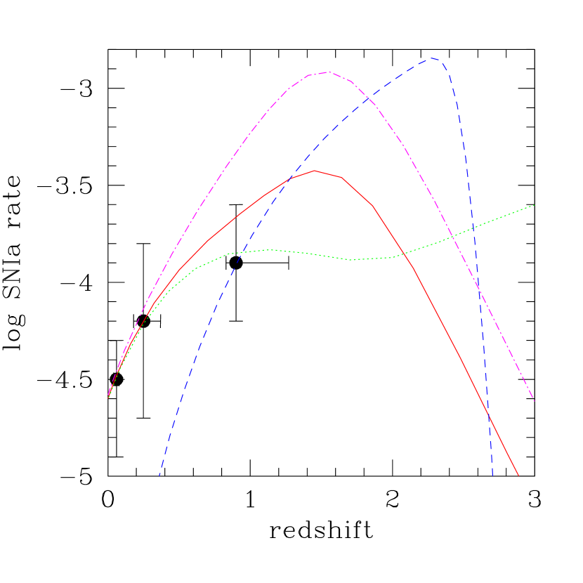
Figure 13: left(a): Evolution of ICM Fe abundance with “naturally” reduced SNIa normalization and $\langle{y_{\rm SNII}}^{\rm Fe}\rangle=0.1~{}{\rm M}_{\odot}$. In hybrid star formation history models, $\alpha_{3X}=1.05$, $z(t_{\rm form})=10$, and $t_{cX}=3$ (2H1.05WxSn; solid curve) or 0.5 Gyr (2H1.05WxStn; dotted curve); in the rapid star formation model, $\alpha_{3X}=1.05$, $z(t_{\rm form})=3,$ and $t_{cX}=0.5$ Gyr (2R1.55Stnz; dashed curve). For comparison, the evolution for model 2H1.05Wx from Figure 7a is re-plotted (dot-dashed curve). right(b): Same as (a) for SNIa rate (in $\delta^{-1}~{}{\rm Mp}c^{-3}~{}{\rm yr}^{-1}$) history.

In order for these models with reduced early SNIa enrichment to match the $z>0.3$ ICM Fe abundance evolution as well as, e.g., the models presented in Figures 11a and 12a, an increase in mean SNII Fe yield to (at least) $\langle{y_{\rm SNII}}^{\rm Fe}\rangle=0.10~{}{\rm M}_{\odot}$ is required (Figure 13a). Because the early ICM Fe enrichment is now dominated by SNII, the ICM Fe evolution is less sensitive to the choice of $t_{cX}$ (for $\langle{y_{\rm SNII}}^{\rm Fe}\rangle=0.07~{}{\rm M}_{\odot}$, the fall-off of ICM Fe with redshift in 2H models is steeper if $t_{cX}=3$ Gyr than if $t_{cX}=0.5$ Gyr). Since the differences in the SNIa rate history emerge beyond the redshift where observed constraints are available (Figure 13b), the SNIa delay time in clusters is unconstrained by observations if the rapid star formation in cluster galaxies was characterized by a flat IMF and high SNII Fe yields. Note that with most of the Fe enrichment due to SNII in the rapid star formation mode, an extended outflow phase is no longer required – provided that the initial ISM fraction, $f_{\rm ISM}({t_{\rm form}})$, is large (e.g., model 2R1.55Stnz). Inclusion of a prolonged outflow period reduces the required value of $f_{\rm ISM}({t_{\rm form}})$.

3.1.6 Model Result Overview

A simple model for the chemical evolution of Fe in the universe may be constructed using parameters drawn from the observed star formation, and Type II and Type Ia supernova, rates in the field population of galaxies that are mutually consistent for a standard IMF. For Fe yields of $0.07~{}{\rm M}_{\odot}$ per SNII and $0.7~{}{\rm M}_{\odot}$ per SNIa, the baryons in the universe are enriched to an average Fe abundance of 0.13 solar. The universal ratio of galactic-to-intergalactic baryons constrains the fraction of Fe locked up in stars and cold gas such that stellar Fe abundances are within a factor of two of solar with the precise value dependent on the magnitude and timing of galactic outflows. The prolonged epoch of star formation coupled with the SNIa delay shifts much of the Fe enrichment to relatively recent ($z<1$) epochs, as indicated by recent observations (Lamareille et al., 2006).

If one naively assumes that rich galaxy clusters are pure representative samples of the universe, this global chemical evolution model directly scales to clusters and Fe abundances in the ICM are badly underestimated. However, in order to better understand the differences in the nature of star formation in cluster and field galaxies, it is instructive to adopt the field model as a point of departure for investigating the variations that are required to reproduce observed $z\approx 0$ Fe abundances of $\sim 0.4$ solar and mild ($z=0-1$) ICM Fe abundance evolution.

Successful variations must include shifts to both higher redshift in the peak of the star formation rate, and to flatter high mass slopes in the IMF for star formation at high redshift – implying that conversion of gas into stars is, on average, more efficient in rich clusters than in the field.

Overall Fe enrichment originates in roughly comparable fractions from SNIa and SNII for models where the relationship between SNIa and star formation is the same in clusters and the field. Due to the long SNIa delay, outflow of Fe from galaxies extends beyond the epoch of rapid star formation in order to be incorporated into the ICM; however, if the outflow is too prolonged, ICM enrichment is too recent and in conflict with the mild observed Fe evolution (see discussion in §4.2 below). The implied SNIa rates at $z\sim 1$ are somewhat at odds with observational limits for clusters, although the conflict is slightly weaker than inferred by Maoz & Gal-Yam (2004) (see discussions in §§4.3 and 4.6 below). Unfortunately, there is as yet no data to provide a more definitive test by offering a comparison with the very high $z=1-2$ cluster SNIa rates predicted by these models (see Figure 7b; Maoz & Gal-Yam 2004).

Additional models with SNIa rate histories that differ from those above, and that generally improve the match to the $z<1$ evolution in ICM Fe inferred from X-ray data, are constructed by (1) shortening the mean delay time in the kernel that transforms the star formation into the SNIa rate, (2) decreasing the initial star formation redshift in models where all stars form in rapid mode, or (3) reducing the number of SNIa explosions per unit mass of stars formed according to the number of intermediate mass ($3-8~{}{\rm M}_{\odot}$) stars whilst increasing the average SNII Fe yield to $0.1~{}{\rm M}_{\odot}$. The SNIa evolution in models of these type, with both rapid and normal star formation modes, most closely reproduce the observed $z<1$ supernova rates. Observations of rapid build-up of Fe, and relatively low $z<1$ star formation and SNIa rates, in clusters are most readily explained in models where heavy element enrichment traces star formation.

4 Discussion, Implications, Predictions

4.1 The IGM Versus the ICM

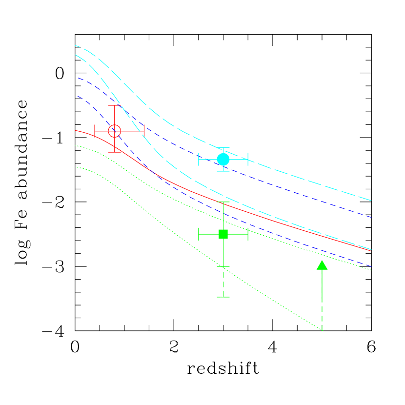
Figure 14: Evolution of the average baryon (solid curve), IGM (dotted curves), stellar (short-dashed curves), and ISM (long-dashed curves) standard model Fe abundances for the “maximum wind” (IGM: upper curve, stars/ISM: lower curve) and “intermediate” cases shown in Figures 4 and 5. The arrow denotes the $z=5$ Ly$\alpha$ forest lower limit from Songaila (2001); the solid square with errorbars the range of $z=2.5-3.5$ Ly$\alpha$ forest measurements from Schaye et al. (2003); Simcoe, Sargent, & Rauch (2004), and references therein; the solid circle the $z=2.5-3.5$ damped Ly$\alpha$ value with errorbars reflecting the uncertain dust depletion fraction of Fe from Pettini (2004) and references therein; and, the open circle with errorbars the $z=0.4-1.5$ damped Ly$\alpha$ systems measurement from Rao et al. (2005). The downward broken extensions for the Ly$\alpha$ forest limits make allowances for the possibility of an $\alpha$/Fe abundance ratios as high as 3:1.

It is valuable to compare, in more detail, observed constraints on the chemical evolution of the universe outside of clusters with the standard model of §2, i.e. a model with star formation history, stellar mass buildup, and Type II and Type Ia supernova rate histories as observed in the field, and with standard IMF and SNII and SNIa Fe yields. Such an examination yields insights into the chemical evolution of the universe, and reveals distinctions from that peculiar to galaxy clusters. Comparisons for the abundance evolution to $z=6$ of the stellar, ISM, and IGM components are shown in Figure 14. Allowing for an Fe-to-$\alpha$-element ratio as low as one-third, the IGM abundance evolution in models with wind parameter greater than that corresponding to $\Omega_{\rm ISM}({t_{\rm form}})>0.0076$ (see middle curves in Figure 4 and 5) is consistent with the $z=5$ Ly$\alpha$ forest lower limit (Songaila, 2001), and with $z=2.5-3.5$ Ly$\alpha$ forest measurements (Schaye et al., 2003; Simcoe, Sargent, & Rauch, 2004). This implies that $>9$% of the $z=0$ IGM originates in galaxies and that the average stellar Fe abundance at $z=2.5$ is $\sim 0.05-0.1$ relative to solar.

The model Fe abundance averaged over all baryons is also consistent with that measured in damped Ly$\alpha$ systems at $z=0.4-1.5$ (argued by Rao et al. 2005 as dominating the mean cosmic metallicity in this redshift interval). The model ISM abundances are consistent with the $z=2.5-3.5$ damped Ly$\alpha$ measurement if $\Omega_{\rm ISM}({t_{\rm form}})<0.028$. The standard model (without an altered IMF, a temporally extended wind, or adjustment of relative normalizations, delays, or yields for supernovae) is in general agreement with all $z>2$ non-cluster metallicity observations (see, also, Daigne et al. 2005).

Note that, at least for Fe, there is no evidence of the missing metal problem summarized in, e.g., Pettini (2004): the models that assume the empirical $z>2.5$ star formation rate are in accord with the observations. There are two factors at play here. The primary one is that, although the Fe yield per star averaged over a Hubble time is indeed $\sim 1.3$ solar as generally assumed, the average yield prior to $z=2.5$ is only $\sim 0.6$ (see Figure 4) due to the delay in SNIa element production. The second factor is that the total ISM density must exceed the value measured in damped Ly$\alpha$ systems, $\Omega_{\rm DLA}(z=2.5)\sim 0.0015$ (Prochaska & Herbert-Fort, 2004). The amount of potentially star-forming gas must be sufficient to account for the stars formed over $z=0-2.5$: $\Omega_{\rm ISM}(2.5)>0.0027$, taking mass return into account and assuming a standard IMF. If one also accounts for the mass loss from the ISM necessary to account for the metals observed in the IGM, $\Omega_{\rm ISM}(2.5)>0.0052$ is inferred – more than three times the damped Ly$\alpha$ value. Thus, the deficit in the detected amount of metals relative to expectations may be better characterized as a “missing gas (ISM)”, rather than a “missing metal,” problem in the $z\sim 2.5$ universe (see, also, Hopkins, Rao, & Turnshek 2005; Prochaska, Herbert-Fort, and Wolfe 2005).

Conversely, there would be a missing metals problem if the variations considered above needed to explain cluster Fe abundances and its evolution were applied to the field, as these were specifically introduced to produce a prodigious rapid enrichment. Models where half the stars in the field were formed from a flat-IMF, rapid star formation mode with either reduced SNIa delay, or increased SNII yields and suppressed SNIa rate, overpredict $z=2.5$ Fe abundances outside of clusters by $>10$. Star formation is fundamentally different in clusters and the field (see §4.4, below).

A full consideration of limits on departures of the standard model consistent with observations outside of clusters is beyond the scope of this work. Given the above conclusions, it is perhaps surprising that field and cluster galaxy populations are not more distinct in terms of apparent ages, mass-to-light ratios, and abundances/abundance ratios – especially since spheroids dominate the stellar mass in both populations (Bell et al., 2003). A general prediction implied by the successful cluster models presented here is of higher Fe abundances in cluster galaxies compared to the field (even though a higher percentage of Fe is locked up in galaxies in the field – $\sim 60$%, compared to $\sim 40$% in clusters). This effect is mitigated if metals are preferentially lost in outflows associated with the rapid star formation.

4.2 The Magnitude and Timing of Galactic Outflows in Clusters

I find that $>25$% of the ICM must originate in galaxies (i.e the “ISM”) in order for the ICM to be enriched in Fe to 0.4 solar. The combination of (1) observations of the large amount of intracluster Fe and its mild evolution since $z=1$, (2) significant limits on the cluster SNIa rate since $z=1$, and (3) the assumption that Fe in the ICM originates in galaxies that are known to form most of their stars at $z>1$ constrains the amount, epoch, and duration of matter and metal transport from cluster galaxies to the ICM. Thus observations of the evolution of ICM enrichment provide a unique diagnostic of the nature of galactic winds associated with galaxy formation in a dense environment.

Since SNII are more numerous than SNIa at all times for all models (see Figures 10ab, noting the respective scales), they are primarily responsible for the ejection of material from galaxies. The SNII rate (and, hence, SNII Fe enrichment) is proportional to the star formation rate that steeply declines with redshift in cluster galaxies. Because the mass loss rate as implemented in equation (21) is proportional both to the SNII rate and to the mass in interstellar gas that decreases with time as it is consumed by star formation and also lost in galactic winds, it falls even more quickly than the star formation rate – and, more quickly than the interstellar medium is enriched. Therefore a prompt phase of only modestly enriched mass injection into the ICM ensues; and, an additional, more prolonged, outflow (see §3.1.1) must be invoked to transport the necessary Fe into the ICM – even if the SNIa delay time is reduced to 0.5 Gyr. The sole exceptions to this requirement are models where SNII fully dominate the ICM Fe enrichment that may be assumed to undergo prompt and very strong (implying very high initial ISM baryon fractions) outflows, although scenarios with longer duration and milder outflows (lower initial ISM baryon fractions) are also feasible (see §3.1.5). However, in models where the galactic outflow era is overly prolonged, the resulting delay in ICM enrichment leads to an underprediction of the observed ICM Fe abundances at $z>0.3$.

Such an additional extended phase of mass loss may be identified with ram-pressure stripping of galaxies rather than galactic winds, since simulations indicate that this is the dominant ICM enrichment mechanism at $z<1$ (Schindler et al., 2005; Domainko, et al., 2006). In the models presented here with extended outflow, $\sim 25-40$% of the enrichment is due to this phase, compared to $\sim 10-25$% in the simulations. Other possible avenues of prolonging the enrichment timescale include efficient winds from a galaxy subpopulation (perhaps late-type or dwarf galaxies) distinct from that responsible for the prompt outflow phase, or the suppression at early epochs in the conversion efficiency of supernovae energy to the kinetic energy of outflow (e.g., if it were more efficiently radiated as a result of a denser protogalactic environment). Some, but not all, these mechanisms are particular to the rich cluster environment.

4.3 Implications for Supernova Physics and Cosmology

As shown in, e.g., Figure 10b the specific cluster SNIa rate is similar to that in the field out to $z=1$ – the maximum redshift for which observational constraints are available in either environment. The inference, drawn above, that cluster star formation is significantly more efficient then implies – assuming universal SNIa Fe yields – that SNIa must occur less frequently per unit mass of star formed, and/or predominantly explode at $z>1$.

Figures 15ab revisit selected curves from Figures 10b, 11b, 12b, and 13b, focusing on the $z<1.3$ region, and with the SNIa rates on a linear, rather than logarithmic, scale. The solid lines show models with standard SNIa normalizations and DTDFs. These are in marginal agreement with the observed cluster rate, and predict an order of magnitude increase just beyond the highest observed redshift bin.

For the hybrid star formation models, decreasing the mean delay time or the number of SNIa per star formed according to the IMF improves the match to the observations and results in less extreme behavior just beyond $z=1$ (Figure 15a), while simultaneously providing models that more precisely fit the ICM Fe data (assuming, in the reduced-normalization models, that the SNII Fe yield is $>0.1~{}{\rm M}_{\odot}$). In contrast, the SNIa rate in models where star formation exclusively occurs in rapid star formation mode generally decline too steeply at low redshift.

There is independent justification for characterizing SNIa explosions associated with the rapid star formation in cluster galaxies with relatively short delay times. Physically plausible double degenerate binary system progenitor models for SNIa with short delay times (Belczynski, Bulik, & Ruiter, 2005) apparently find realization in regions of active star formation. Evidence includes the measurement of higher SNIa rates in blue, relative to red, galaxies (Mannucci et al., 2005); and, of higher rates in early-type galaxies when they are radio loud (Della Valle et al., 2005). This is consistent with the observation of systematic differences in the characteristics of individual SNIa in elliptical and spiral galaxies (Della Valle et al. 2005, Garnavich & Gallagher 2005). Finoguenov et al. (2002) also suggested that multiple SNIa types are required based on gradients in abundance ratios in the ICM. High and persistent Fe abundances, and Fe-to-$\alpha$ ratios, in the nuclei of galaxies hosting high redshift quasars also may indicate the presence of short-delay-time SNIa (Dietrich et al. 2003, Maiolino et al. 2003). The successful models presented here with reduced SNIa delay times in the rapid star formation mode fit in well with these observations, providing a connection between star formation in local galaxies and the starbursts responsible for the elliptical galaxy stellar populations that dominate in rich clusters. I have shown that, if the SNIa per star formed in such models is determined by renormalizing the field value according to the relative number of $3-8~{}{\rm M}_{\odot}$ stars, then the SNII Fe yield must exceed $0.1~{}{\rm M}_{\odot}$ irregardless of the rapid mode mean SNIa delay time. However, one need not assume that progenitors of the two proposed subclasses of SNIa explode with the same likelihood (Mannucci et al., 2006).

Even for a given progenitor model, the distribution of delay times is sensitive to the distribution of orbital separations and mass ratios, and other factors, that depend on the initial mass function and galaxy age and metallicity in a complex and uncertain manner (Greggio, 2005). Moreover, the evidence for a 3 Gyr mean delay for SNIa in the field has recently been questioned (Barris & Tonry, 2006). Given these considerations, in combination with uncertainties in the configuration of SNIa progenitors and explosion mechanism, one hesitates to suggest that the possibility that rapid star formation produce SNIa with shorter delay times casts doubt on the utility of SNIa as standard candles (Yungelson & Livio, 2000). In any case, since models where SNII dominate Fe enrichment are not ruled out, the evolution of intracluster Fe does not constrain the SNIa delay time in a model-independent way. Additional consideration of abundance ratios, and particularly their evolution, may be more definitive.

4.4 The Efficiency and Nature of Star Formation in Cluster Galaxies Compared to Field Galaxies

The baryon mass fraction in stars, $f_{\rm b,stars}$ and star-to-gas ratio, $f_{\rm b,stars}/f_{\rm b,gas}$, in rich galaxy clusters may be estimated from several recent observational studies – although uncertainties persist. Estimates of the total B-band mass-to-light ratio cluster around $300~{}{\rm M}_{\odot}/{\rm L}_{{\rm B}\odot}$ with a spread of $\sim 30$% (Marinoni & Hudson, 2002; Girardi et al., 2002; van den Bosch, Yang, & Mo, 2003; Sanderson & Ponman, 2003), while the stellar mass-to-light ratio for a composite stellar population dominated by old stars to the degree appropriate for clusters is $\sim 4.5~{}{\rm M}_{\odot}/{\rm L}_{{\rm B}\odot}$ (Marinoni & Hudson 2002; note, however, that this assumes a standard IMF). This yields a mass fraction in stars of $\approx 0.015$ and $f_{\rm b,stars}/f_{\rm b,gas}=1/8$ (assuming a cluster baryon bias factor of 0.9) – roughly twice the universal ratios. Similar ratios are derived from estimates of the total (Kochanek et al., 2003) and stellar (Drory et al., 2004) mass-to-light ratios where luminosities are measured in the K-band (see, also, Lin, Mohr, & Stanford 2003).

The overall implications of these estimates of baryon mass fractions in stars for galaxy clusters that significantly exceed the universal value, and their connection to the problem of elemental abundances in the ICM, may not be fully appreciated. The modeling approach presented here provides a quantitative perspective on some of the distinctions between star formation in the field and in clusters that complements studies of stellar populations. In models that successfully reproduce observed $z=0-1$ ICM Fe abundances, a significant fraction of the current mass in cluster galaxy stars forms in a rapid mode of star formation characterized by a top-heavy IMF. The properties of the populations of Lyman-break and submillimeter galaxies provide independent evidence for such an IMF in the environments of rapid merger-driven star formation at high redshift of the kind that dominates in cluster galaxy progenitors (Baugh et al., 2005). Because of the higher return fraction in this component, more than two-thirds of the integrated star formation occurs in this mode, in accord with the large fraction of cluster stellar mass residing in early-type systems (Goto et al., 2003; Postman et al., 2005), and the high formation redshift (Blakeslee et al., 2004; Holden et al., 2004; Cimatti et al., 2004; van Dokkum et al., 2004; Chen & Marzke, 2004; Thomas et al., 2005; Longhetti et al., 2005) and relatively small amount of continuing star formation (Jørgensen et al., 2005; Thomas et al., 2005; Romeo, Portinari, & Sommer-Larsen, 2005) in cluster galaxies. The inferred mass return fraction is $\sim 70$%, compared to 40% for a standard IMF, implying that star formation would be 2–3 times more efficient than would be the case for a standard IMF even assuming the same present-epoch stellar mass fraction. If the baryon fraction in stars at $z=0$ is indeed twice as high in clusters as in the field, and stars form in field galaxies with a predominantly standard IMF, then star formation in clusters is 3 – 5 times more efficient. Likewise, $\sim 25-35$% of cluster baryons may be inferred to be cycled through stars (this fraction is $\sim 10$% for the standard model). Moreover, although the mass fraction of stars formed that is currently locked up in stellar remnants is $\sim 13-15$%, $\sim 40-60$% of the stellar mass today is in that, non-luminous, form (compared to $\sim 20$% for a standard IMF).

These inferences have implications for constructing and interpreting population synthesis models of cluster galaxies, and for estimating their stellar mass-to-light ratios (e.g., Zepf & Silk 1996), as well as for evaluating the extent and nature of “overcooling” and feedback in numerical simulations of cluster formation (Balogh et al., 2001; Kravtsov, Nagai, & Vikhlinin, 2005). It is crucial not to neglect mass return in inventories of the integrated star formation, especially in clusters.

Most, but not all, cluster star formation is required to occur at high redshift. As discussed in the previous section, models that provide the best simultaneous fits to the SNIa rate and ICM Fe evolution are those with hybrid star formation histories, since the SNIa rate steeply declines at $z<1$ in models where star formation exclusively originates in rapid mode. This may be taken as an indication that the finite (if small) low-redshift cluster SNIa rates imply a non-negligible degree of relatively recent star formation activity in cluster galaxies. While the Butcher-Omeler effect indicates that recent epoch star formation is suppressed relative to the field by a factor of $>10$ in rich cluster cores, star formation persists outside of the core where late-type galaxies are more common (Bai et al., 2006). In any case, since the estimated low-$z$ cluster SNIa rate is only $3\sigma$ above 0, it is likely that one could construct hybrid-SFH models with a lower level of recent ($z<0.5$ – considering the delay in SNIa enrichment) star formation than in those presented here that would be equally successful – particularly if one considers a SNIa delay time distribution function that falls off less steeply at long delays than the Gaussian function considered here. In fact, if there are two subpopulations of SNIa, with DTDFs centered on short ($<<10^{9}$ yr) and long ($>10^{9}$ yr) delays, respectively, an exponential distribution for the long-delay SNIa provides a better fit to the observed field SNIa rate history (Mannucci et al., 2006).

4.5 Origin and Enrichment History of Intracluster Fe

In the models that, simultaneously, best match the ICM Fe abundance and SNIa rate evolution, ICM enrichment traces star formation via either a combination of SNII and short-time-delay SNIa (2H1.05WxSt1, 2H1.05WxSt2; Figure 11), or domination by SNII (2H1.05WxSn, 2H1.05WxStn; Figure 13). For the former, the fraction of stars in SNIa progenitors is assumed to be the same as for a standard IMF, even though the total fraction of stars in the $3-8~{}{\rm M}_{\odot}$ range is lower. Under the IRA, the integrated SNIa Fe enrichment per baryon, relative to solar, is

$${\langle{\rm Fe}\rangle}_{\rm bar}({\rm SNIa})=\left({0.097\over{1-R}}\right)\left({{{y_{\rm SNIa}}^{\rm Fe}}\over{0.7~{}{\rm M}_{\odot}}}\right)\left({{f_{\rm stars}^{\rm total}}\over{0.12}}\right)\left({{\nu}\over{1.5\ 10^{-3}{\rm SNIa}\ {{\rm M}_{\odot}}^{-1}}}\right),$$ (23)

where, ${f_{\rm stars}^{\rm total}}=f_{\rm stars}+f_{\rm Xstars}$ is the total present-day stellar baryon fraction. The cluster value inferred from observations is

$${\langle{\rm Fe}\rangle}_{\rm bar}({\rm OBS})=0.346\left({{f_{\rm ICM}}\over{0.865}}\right)\left({{\langle{\rm Fe}\rangle}_{\rm ICM}\over{0.4}}\right)+0.135\left({{1-f_{\rm ICM}}\over{0.135}}\right)\langle{\rm Fe}\rangle_{\rm gal},$$ (24)

where $f_{\rm ICM}$ is the cluster baryon fraction contained in the ICM; $f_{\rm ICM}=0.865$ corresponds to $f_{\rm stars}^{\rm total}=0.12$. For $\langle{\rm Fe}\rangle_{\rm gal}=1-3$ (the successful models here predict values at the higher end of this range), ${\langle{\rm Fe}\rangle}_{\rm bar}({\rm OBS})\approx 0.5-0.75$.

${\langle{\rm Fe}\rangle}_{\rm bar}({\rm SNIa})$ is calculated, without assuming the IRA, and plotted in Figures 16ab as a function of rapid star formation IMF slope ($\alpha_{3X}$), assuming $m_{DX}=m_{D}=2~{}{\rm M}_{\odot}$, $\alpha_{3}=2.3$, $z(t_{\rm form})=10$, $f_{\rm stars}^{\rm total}=0.12$, and ${y_{\rm SNIa}}^{\rm Fe}=0.7~{}{\rm M}_{\odot}$. Evidently, SNIa synthesize a significant fraction of cluster Fe only in models characterized by a flat IMF, and with $\nu$ maintained at its value deduced in the field. Moreover, the SNIa Fe yield must be high. While recent multi-dimensional simulations (Travaglio et al., 2004; Röpke et al., 2005) predict lower yields, phenomenological studies continue to favor higher values of ${y_{\rm SNIa}}^{\rm Fe}$ (Badenes et al., 2006).

Similarly, the integrated SNII Fe enrichment per baryon, assuming IRA, is

$${\langle{\rm Fe}\rangle}_{\rm bar}({\rm SNII})=\left({0.065\over{1-R}}\right)\left({{{y_{\rm SNII}}^{\rm Fe}}\over{0.07~{}{\rm M}_{\odot}}}\right)\left({{f_{\rm stars}^{\rm total}}\over{0.12}}\right)\left({{K_{\rm SNII}\over{10^{-2}{\rm SNII}}\ {{\rm M}_{\odot}}^{-1}}}\right).$$ (25)

Figures 16ab also include the computation, without assuming the IRA, of ${\langle{\rm Fe}\rangle}_{\rm bar}({\rm SNII})$ for the parameters listed above and ${y_{\rm SNII}}^{\rm Fe}=0.07~{}{\rm M}_{\odot}$, as well as the summed SN Fe enrichment per baryon. In addition, the local IMF slope, and range of ${\langle{\rm Fe}\rangle}_{\rm bar}({\rm OBS})$ estimated above, are indicated. These figures emphasize the robustness of the requirement for a flat IMF (unless ${y_{\rm SNII}}^{\rm Fe}>0.2~{}{\rm M}_{\odot}$), and illustrate the challenge in producing sufficient Fe in the hybrid star formation models (that best match the observed cluster SNIa evolution) if the SNIa progenitor probability for stars in the $3-8~{}{\rm M}_{\odot}$ range is universal. The Fe enrichment per baryon for such models plateaus at $\sim 0.55$, explaining why ${y_{\rm SNII}}^{\rm Fe}=0.1~{}{\rm M}_{\odot}$ (or greater) is favored if $\nu$ is scaled in this manner (§3.1.5).

To summarize, the observed frequency of SNIa in clusters (or in the universe as a whole) is insufficient to account for cluster Fe enrichment. Therefore, either a separate class of prompt, high Fe yield SNIa that initiate at high redshift explode with an incidence per star formed that exceeds what one expects based on the field value and relative number of $3-8~{}{\rm M}_{\odot}$ stars, or the shortfall is made up by SNII. These SNII must primarily originate from rapid star formation with a flat IMF, and yield an average of $>0.1~{}{\rm M}_{\odot}$ of Fe. If this is the case, SNII dominate cluster enrichment, implying a SNII-like pattern of elemental abundances in the ICM and in the oldest cluster galaxies. This pattern is fixed at high redshift, unlike its counterpart in field galaxies where Fe enrichment is delayed. Enhanced numbers of SNII, and likely gamma-ray bursts as well, in clusters at $z>1.5$ are then expected.

4.6 Additional Notes on Similar Studies

Maoz & Gal-Yam (2004) reached similar conclusions with regard to the inadequacy of SNIa, and the likely need for a top-heavy IMF, to account for ICM Fe. Their approach was essentially as follows. They calculated the number of SNIa required to make up the Fe deficit left after subtracting the SNII contribution – assuming a Salpeter IMF ($\alpha_{0}=\alpha_{1}=\alpha_{2}=\alpha_{3}=2.35$) – from what is observed at $z=0$. They then distribute those SNIa in redshift according to a particular formation epoch $t_{\rm form}$ and SNIa delay time distribution – assuming that all stars formed in a burst at $t_{\rm form}$ – for comparison with the cluster SNIa rate evolution derived from their observations. In agreement with the present work, they find that the specific incidence of SNIa progenitors required exceeds the field value by an order of magnitude. Assumptions in their analysis that differ from the present one include (1) $z(t_{\rm form})=2$ or 3, (2) a pure instantaneous burst, (3) a lower stellar mass-to-light ratio (implicitly), (4) neglect of the difference between the mass of stars formed over a Hubble time and that measured at $z=0$. In addition, Maoz & Gal-Yam (2004) adopt a SNIa delay time distribution that is both more sharply peaked and with a more prominent tail to long delays. Nevertheless, their results are broadly consistent with those presented here in marginally allowing scenarios where $z(t_{\rm form})=3$ and the mean delay time is 3 Gyr (Figure 12). The present study goes further in explicitly considering a range of IMFs and possible star formation and outflow histories to calculate the evolution of ICM enrichment, and in concluding that models with more prompt enrichment more accurately predict the flat ICM Fe evolution that is observed.

Portinari et al. (2004) analyzed the cluster metal inventory at $z=0$. An instantaneous burst of star formation was assumed, with self-consistent treatment of the stellar mass-to-light ratio and mass return, although the stellar Fe abundance was put in by hand. Since chemical evolution is not modeled, the observed ICM Fe evolution is not utilized to evaluate scenarios. Models with top-heavy IMFs or non-standard SNIa parameters were not explicitly considered. Nevertheless, their rejection of a standard IMF is robust and in agreement with the conclusions presented here.

De Lucia, Kauffmann, & White (2004) utilized N-body simulations in a $\Lambda$CDM universe, conjoined with a parameterized semi-analytic treatment of astrophysical processes in the baryonic component such as cooling, star formation, feedback, and galactic winds, to simulate the chemical evolution of the IGM and the ICM. Yields appropriate to a top-heavy IMF are adopted, although mass return and the photometric properties of galaxies were computed for a Salpeter IMF. In agreement with the results of this work, they found that in models tuned to reproduce the observational properties of $z=0$ galaxies, ICM enrichment was invariably concentrated to high redshifts – a direct result of the $z=5$ peak in the star formation rate and the assumption of instantaneous recycling.

The semi-analytic models of Nagashima et al. (2005a) included a more detailed treatment of chemical evolution, and adopted some of the enhancements listed in §4.7 below, such as a two-phase ISM and separate treatment of galaxy disk and bulge components. They fixed the disk and bulge IMFs, with the latter characterized by a monotonic flat slope (thus maximizing the SNII/SNIa ratio in this population), and also adopt a single prescription for computing the SNIa rate. Neither the star formation, nor the SNIa, rate histories were shown or directly compared to observations; however, the latter seems to have a mean delay intermediate between those most often considered here (i.e. $t_{c}=0.5$, 3 Gyr). Yet again, it was concluded that a top-heavy IMF (corresponding to $\alpha_{3X}=1$) is required to produce sufficient metals – an inference further supported by comparing Fe-to-$\alpha$-element ratios in individual elliptical galaxies with those in galaxy formation simulations (Nagashima et al., 2005b). ICM Fe enrichment of the ICM occurs early in their models, as observed, with $\alpha$-element enrichment ensuing even more promptly.

Contrary to the results of the present investigation, and those described above, Ettori (2005) concluded that ICM Fe can be accounted for by enrichment from star formation with a Salpeter IMF and SNIa with delay time and normalization as found in the field by Strolger et al. (2004) and Dahlen et al. (2004) – similar to model 1N2.3 in the present work that was dismissed as failing to produce adequate Fe. Ettori (2005) acknowledged, however, that not enough stars are observed (via $L_{B}$) for this scenario to be fully coherent. This internal inconsistency can be clarified as follows. The supernova parameters adopted in Ettori (2005) result in an Fe yield of $1.05\ 10^{-3}$ per solar mass of star formation compared to the estimated total cluster Fe mass of $8.6\ 10^{-3}$ per solar mass of ICM – i.e. a mass ratio of stars-formed to gas of 0.82, or a ratio of stars formed to stars observed today of 6.3 (for a present-day cluster star-to-gas ratio of 0.12) is implied. The implied return fraction of 0.84 is grossly inconsistent with the initial assumption of a Salpeter IMF.

4.7 Model Shortcomings and Future Refinements

One might be troubled by the high initial ISM baryon fractions, and the high resulting galactic Fe abundances, in models that best explain the ICM Fe and SNIa observations. The need for a reservoir to provide for the copious ensuing star formation (no additional sources of star-forming gas – via, e.g., infall – are subsequently introduced), and to soak up the newly synthesized metals to be ejected into the IGM drives the requirement for the former. In the context of the simple models constructed here, the latter is an inevitable consequence of the early epoch for most star formation and the observationally-driven requirement for early enrichment. A number of refinements that may prove fruitful in follow-up studies, some of which are relevant to these issues, may be considered.

In the models presented here, star formation and IGM-enriching outflows originate in the same single-component ISM. One may subdivide the ISM into hot and cold phases, with stars exclusively forming from the latter and outflows exclusively originating in the former. The two phases can exchange mass and be distinctly enriched by supernovae. One may alternatively, or additionally, include “bias” parameters to ensure that outflowing and/or star-forming gas is preferentially metal-enriched relative to the average in the ISM. These all may affect the relationship between the required duration of galactic outflows and the amount of metals locked up in stars. Likewise, requirements on the magnitude and timing of outflows may be altered by explicitly considering (re)accretion of IGM onto galaxies. Outflows associated with SNII and SNIa may be “decoupled” by associating distinct normalizations with each type.

The number of components may be further expanded in order to, e.g, allow for separate treatment of bulges and disks within the stellar component as regards star formation rate, IMF, SNIa normalization and delay time distribution, outflows/inflows, etc. – rather than the less physically motivated division into “field-like” and “cluster-enhancement” components. This additional level of detail clarifies the field/cluster dichotomy, and would enable a more detailed evaluation of the star formation histories in the models.

A more sophisticated treatment of supernovae could include yields that depend on progenitor mass, thus introducing an IMF-dependence for average yields, or on the metallicity of the progenitor population. These are often implemented for SNII, but could be considered for SNIa as well, as could a metal dependence of the number of SNIa per star formed.

A less empirical treatment of star formation could be implemented in a global manner by specifying an explicit, parameterized dependence on total ISM mass density constrained by observations of field star formation rates and the distinct stellar inventories in clusters and in the field. An explicit metallicity-dependent IMF could be considered. The formation and evolution of binary star systems may be distinctly and explicitly traced, and granted a role in determining the SNIa rate.

Population III enrichment may be more carefully considered, especially in relation to metal build-up at high-redshift. The overall impact of such a component is generally considered minor in the IGM out to relatively high redshift (Yoshida, Bromm & Hernquist 2004; Norman, O’Shea, & Paschos 2004; but, see Salvaterra & Ferrara 2003), but may be of enhanced significance in clusters (Loewenstein, 2001).

Finally, one should consider the abundance evolution of additional elements, such as O, Mg, and Si to further constrain the combination of IMF, relative SNII/SNIa normalization, and outflow parameters, as well as the average yields themselves.

While the above considerations indicate limitations of the present work, the physically and observationally motivated, self-consistent models constructed here reveal a number of implications and puzzles. By virtue of the simplicity and limited number of free model parameters in this approach, one can draw conclusions and identify persistent paradoxes – summarized in the section that follows – that are qualitatively model-independent and easily traced to particular phenomenon or assumptions.

5 Summary and Concluding Remarks

I constructed models for the coupled mass density and Fe abundance evolution of stars, interstellar (potentially star-forming) gas, and intergalactic (inert) gas in a closed box, with application to the universe as a whole and extension to the special environments of rich clusters of galaxies. I focused on Fe because of its power as a diagnostic of SNIa astrophysics and the unmatched constraints provided by recent observations of the evolution of the SNIa rate and ICM Fe abundance. I adopted empirically based source terms to mitigate the limitations in our understanding of star formation and the physics and astrophysics of supernova explosions. I considered the effects of varying the star formation rate history, initial mass function, SNII Fe yields, SNIa rate normalization and distribution of delay times, and strength and duration of galactic outflow on field and cluster observables. Confrontation of models with observations of the three components in both environments, and over a range in redshift, constrain the mechanisms, and highlight the distinctions, of metal enrichment in the field and in clusters that depend on the physical characteristics of star formation and SNIa explosions.

5.1 Chemical Evolution of Fe in the Universe

The average star formation history in the universe is measured out to redshift $z\sim 6$ (Giavalisco et al., 2004), and a SNIa delay time distribution function derived from a comparison with the SNIa rate history to $z>1$. The results of direct application of these functions – assuming a standard IMF, and standard SNIa and SNII Fe yields – to chemical evolutionary models are consistent with metallicities measured in damped Ly$\alpha$ systems out to $z\sim 3.5$ and in the IGM to $z\sim 5$. A standard IMF also correctly predicts measurements of the buildup of stellar mass over cosmic time, and estimated SNII rates to $z\sim 1$. A careful accounting of star formation, stellar mass return, and galactic winds implies that the ISM density is $>3$ times that in damped Ly$\alpha$ systems (DLAs) at $z=2.5$, supporting suggestions that the “missing metal” problem is actually a “missing gas” problem – i.e. that there is more potentially star-forming gas than currently measured in DLAs. The delay in SNIa enrichment implies that less than 10% of the Fe in field galaxies was in place at $z=2$ and that the Fe yield per star formed at that redshift was approximately half the current value. One expects a negative correlation of the Fe-to-$\alpha$ elemental abundance ratio with stellar population age. Although some field star formation may proceed with a flat IMF (van der Wel et al., 2006), drastic departures from the standard model presented here, unless constructed in a highly contrived manner, are ruled out by observations and their mutual consistency within the standard framework.

5.2 Chemical Evolution of Fe in Clusters

The amount of Fe per baryon measured in clusters exceeds that predicted by the successful and internally consistent field model described above by more than a factor of four. And yet, surveys fail to detect supernovae – in particular SNIa that most efficiently synthesize Fe – in sufficient numbers to account for this hyper-enrichment. In this paper I presented, and evaluated the plausibility and implications of, possible resolutions to this now well-established (Portinari et al. 2005, and references therein) paradox.

Clusters are typically inferred to have roughly twice the stellar mass fraction as in the field, and cluster galaxies are believed to form stars more rapidly. However, these factors are insufficient (although the latter is necessary) for reproducing the observed Fe abundance and its mild evolution since $z\sim 1$. Fe must be synthesized in abundance at an early epoch, and must be efficiently transported from galaxies to the ICM. Therefore, a significant fraction of star formation must proceed rapidly with a top-heavy IMF (see, also, Finoguenov, Burkert, & Böhringer 2003). Star formation is $3-5$ times more efficient in rich clusters than in the field, mitigating the overcooling problem in numerical cluster simulations. Both the fraction of baryons cycled through stars, and the fraction of the total present-day stellar mass in the form of stellar remnants, are substantially greater in clusters than in the field. Assuming that metals are well-mixed in the ISM before ejection, $\sim 40-70$% of the ICM must originate in galaxies (see, also, Moretti et al. 2003), with the lower values generally associated with galactic outflows assumed to continue for longer durations.

Confirming and extending the conclusions drawn by previous studies (see §4.6), I demonstrated that the observed mild amount of evolution in Fe is most accurately reproduced in models where the enrichment tracks star formation, implying that synthesis of cluster Fe was dominated by SNII (if the SNIa rate normalization is scaled down from its value in the field according to the relative number of $3-8~{}{\rm M}_{\odot}$ stars) and/or SNIa with short delay times whose progenitors originated during a phase of rapid, top-heavy star formation (see, also, Scannapieco & Bildsten 2005). In the former, $\geq 0.1~{}{\rm M}_{\odot}$ per SNII is required; in the latter $\geq 10^{-3}~{}{\rm M}_{\odot}$ of Fe from SNIa per star formed is required.

The best matches to the low observed $z<1$ cluster SNIa rates are reproduced in models where cluster star formation does not exclusively occur at high redshift, but continues to at least $z\sim 0.5$. This is a more prolonged history of star formation than inferred in the central regions of rich clusters, and is contingent on the assumption of a steep decline in the SNIa delay time distribution function beyond 3 Gyr.

Observations of high Fe content in the ICM and its persistence to $z=1$, in combination with constraints on SNIa enrichment from rates measured to similar redshifts, confirms the rapid and efficient nature of star formation in galactic spheroids in clusters, and provides overwhelming evidence that this star formation was characterized by a top-heavy IMF that produced Type Ia less efficiently and/or with shorter delay times (on average) than in field galaxies. Rich galaxy clusters are, indeed, special environments and should only be treated as “fair samples of the universe” in a limited and well-defined context.

Table 1: Model Input Parameters

model	$f_{\rm stars}$	$\alpha_{3}$	$f_{\rm Xstars}$	$m_{DX}$	$\alpha_{3X}$	${{t_{\rm wind}}\over{t_{\rm now}}}$	${{\Delta t_{\rm wind}}\over{t_{\rm now}-t_{\rm form}}}$	$f_{\rm ISM}({t_{\rm form}})$	$t_{c}$	$t_{cX}$
1N2.3	0.059	2.3	0	$\cdots$	$\cdots$	$\cdots$	$\cdots$	0.35	3.0	$\cdots$
1N1.05Wc	0.059	1.05	0	$\cdots$	$\cdots$	$\cdots$	0.5	0.38	3.0	$\cdots$
1H0.8Wc	0.029	1.8	0.029	0.5	0.8	$\cdots$	0.5	0.38	3.0	3.0
1R1.05Wc	0	$\cdots$	0.059	2.0	1.05	$\cdots$	1.0	0.32	3.0	3.0
2H0.8Wc	0.059	2.3	0.059	8.0	0.8	$\cdots$	0.66	0.34	3.0	3.0
2H1.05	0.059	2.3	0.059	2.0	1.05	$\cdots$	$\cdots$	0.48	3.0	3.0
2H1.05Wx	0.059	2.3	0.059	2.0	1.05	1.0	$\cdots$	0.52	3.0	3.0
2H1.3Wx	0.059	2.3	0.059	2.0	1.3	0.5	$\cdots$	0.51	3.0	3.0
2H1.3Wc	0.059	2.3	0.059	2.0	1.3	$\cdots$	1.0	0.34	3.0	3.0
2H1.55Wx	0.059	2.3	0.059	0.5	1.55	1.0	$\cdots$	0.68	3.0	3.0
2R1.55Wx	0	$\cdots$	0.12	2.0	1.55	1.0	$\cdots$	0.50	$\cdots$	3.0
2H1.05WxSt1	0.059	2.3	0.059	2.0	1.05	1.0	$\cdots$	0.51	0.5	0.5
2H1.05WxSt2	0.059	2.3	0.059	2.0	1.05	1.0	$\cdots$	0.51	3.0	0.5
2R1.55WxSt	0	$\cdots$	0.12	2.0	1.55	1.0	$\cdots$	0.50	$\cdots$	0.5
2R1.55WxSz	0	$\cdots$	0.12	2.0	1.55	1.0	$\cdots$	0.83	$\cdots$	3.0
2R1.55WxStpz	0	$\cdots$	0.12	2.0	1.55	1.0	$\cdots$	0.75	$\cdots$	1.5
2R1.55WxStz	0	$\cdots$	0.12	2.0	1.55	1.0	$\cdots$	0.58	$\cdots$	0.5
2H1.05WxSn	0.059	2.3	0.059	2.0	1.05	1.0	$\cdots$	0.60	3.0	3.0
2H1.05WxStn	0.059	2.3	0.059	2.0	1.05	1.0	$\cdots$	0.60	3.0	0.5
2R1.55Stnz	0	$\cdots$	0.12	2.0	1.55	$\cdots$	$\cdots$	0.73	$\cdots$	0.5

Table 2: Model Characteristics and Results at $z=0$

model	$\dot{n_{\rm SNII}}$	$\dot{n_{\rm SNIa}}$	$f_{\rm Ia}{\rm(Fe)}$	${y^{\rm Fe}}_{\rm stars}$	${\langle{\rm Fe}\rangle}_{\rm bar}$	${\langle{\rm Fe}\rangle}_{\rm IGM}$	${\langle{\rm Fe}\rangle}_{\rm gal}$
1N2.3	0.59	0.25	0.58	1.3	0.13	0.056	1.0
1N1.05Wc	3.7	0.84	0.42	1.8	0.59	0.41	2.8
1H0.8Wc	0.76	0.19	0.45	1.8	0.51	0.39	1.9
1R1.05Wc	0.019	0.015	0.44	1.8	0.61	0.43	2.8
2H0.8Wc	0.60	0.26	0.53	1.5	0.50	0.38	1.3
2H1.05	0.61	0.26	0.46	1.7	0.74	0.26	3.8
2H1.05Wx	0.61	0.26	0.46	1.7	0.74	0.36	3.2
2H1.3Wx	0.61	0.26	0.45	1.8	0.62	0.40	2.1
2H1.3Wc	0.61	0.26	0.45	1.8	0.62	0.42	1.9
2H1.55Wx	0.61	0.26	0.43	1.7	0.66	0.35	2.6
2R1.55Wx	0.023	0.017	0.43	1.9	0.73	0.37	3.0
2H1.05WxSt1	0.61	0.099	0.46	1.7	0.74	0.40	2.9
2H1.05WxSt2	0.61	0.25	0.46	1.7	0.74	0.40	2.9
2R1.55WxSt	0.023	0.0024	0.43	1.9	0.73	0.39	2.9
2R1.55WxSz	0.077	0.058	0.43	1.9	0.72	0.40	2.8
2R1.55WxStpz	0.077	0.018	0.43	1.9	0.73	0.40	2.8
2R1.55WxStz	0.077	0.0083	0.43	1.9	0.73	0.40	2.8
2H1.05WxSn	0.61	0.025	0.20	1.7	0.71	0.40	2.7
2H1.05WxStn	0.61	0.025	0.20	1.7	0.71	0.41	2.7
2R1.55Stnz	0.077	0.0055	0.25	2.1	0.80	0.40	3.4

Note. — Supernova rates, $\dot{n_{\rm SNII}}$ and $\dot{n_{\rm SNIa}}$ are in units of $10^{-4}$ $Mpc^{-3}yr^{-1}\delta^{-1}$, where $\delta$ is the baryon overdensity; $f_{\rm Ia}{\rm(Fe)}$ is the fraction of Fe originating from SNIa, ${y^{\rm Fe}}_{\rm stars}$ the Fe yield per star relative to the solar mass fraction; ${\langle{\rm Fe}\rangle}_{\rm bar}$ the Fe produced per total baryon; ${\langle{\rm Fe}\rangle}_{\rm IGM}$ and ${\langle{\rm Fe}\rangle}_{\rm gal}$ the average Fe abundances in the ICM/IGM and in galaxies, respectively.

Figure 1: Integrated return fraction as a function of IMF slope above $m_{D}$ for $m_{D}=0.5$, 1, 2, 4, and $8~{}{\rm M}_{\odot}$ (solid, short-dash, long-dash, dot–short-dash, and dot–long-dash line-type, respectively).

Figure 2: Bell (2005) (solid curves) and Strolger et al. (2004) (broken curves) star-formation rate (in ${\rm M}_{\odot}~{}{\rm Mp}c^{-3}~{}{\rm yr}^{-1}$) history parameterizations for $m_{D}=1~{}{\rm M}_{\odot}$ and (top to bottom) $\alpha_{2}=0.3$, 1.3, 2.3, and 2.8. The rates are renormalized to yield the measured present-day stellar density when integrated over time. (Fukugita & Peebles, 2004).

Figure 3: left(a): Type II supernova rate (in ${\rm Mp}c^{-3}~{}{\rm yr}^{-1}$) evolution corresponding to the curves in Figure 2. right(b): Type II supernova rate evolution for Bell (2005) star-formation history parameterizations for $\alpha_{2}=0.3,1.3,2.3$, and 2.8 (solid, dot, short-dash, and long-dash line-type respectively). For $\alpha_{2}=0.3$ and 1.3, the upper (lower) curves denote $m_{D}=1~{}{\rm M}_{\odot}$ ($m_{D}=8~{}{\rm M}_{\odot}$); this is reversed for $\alpha_{2}=2.8$. The histogram shows the observed SNII rates from Dahlen et al. (2004) for the redshift intervals $z=0.1-0.5$ and $0.5-0.9$ and the field rate from Cappellaro, Evans, & Turatto (1999) for $z<0.1$ (converted using a mass-to-blue-light ratio of 2.4; Fukugita & Peebles 2004); estimated uncertainties are at the $\sim 50$% level.

Figure 4: left(a): Evolution of stellar Fe abundance for the standard (see text) model. The cases with no wind ($\Omega_{\rm ISM}({t_{\rm form}})\equiv\rho_{\rm ISM}({t_{\rm form}})/\rho_{\rm crit}=\Omega_{\rm stars}({t_{\rm now}})+\Omega_{\rm ISM}({t_{\rm now}})=0.0034$), maximum wind ($\Omega_{\rm ISM}({t_{\rm form}})=\Omega_{b}-\Omega_{\rm III}\approx 0.045$) and an intermediate case ($\Omega_{\rm ISM}({t_{\rm form}})=0.0076$) are denoted by long-dash, dot, and short-dash line-type, respectively. The upper solid curve shows the Fe yield per unit star formed (relative to the solar Fe mass fraction), the lower solid curve the overall average abundance (or, equivalently, yield per baryon). right(b): Same as (a) for the ISM Fe abundance.

Figure 5: Same as Figure 4 for the IGM Fe abundance (the abundance is 0 for the no-wind case).

Figure 6: Ratio of galactic Fe abundance to ICM Fe abundance as a function of the present-day mass fraction of Fe in the ICM for overall ICM mass fractions 0.924 (solid curve), 0.865 (dotted curve), and 0.806 (dashed curve) – corresponding to baryon fractions in stars equal to the universal value, twice the universal value, and three times the universal value, respectively (the universal value for the ISM baryon fraction is assumed).

Figure 8: left(a): Evolution of ICM Fe abundance for Model 2H1.3Wx with variations in $K_{\rm GW}$ ranging from its minimum to maximum allowed value. These correspond to initial ISM baryon fractions, $f_{\rm ISM}({t_{\rm form}})=0.30$, 0.37, 0.44, 0.51, 0.58, 0.65, 0.72, 0.79, 0.86, 0.93, and 1.0 (lower to upper curves). The $f_{\rm ISM}({t_{\rm form}})=0.51$ curve is also plotted in Figures 7a and 7b. right(b): Same as (a) for galactic abundance (with lower curves corresponding to smaller values of $f_{\rm ISM}({t_{\rm form}})$). The stellar Fe abundance evolution is shown by the broken line.

Figure 15: left(a): SNIa rate (in $10^{-4}~{}\delta^{-1}~{}{\rm Mp}c^{-3}~{}{\rm yr}^{-1}$) for Models 2H1.05Wx (solid curve), 2H1.05WxSt1 (dotted curve), 2H1.05WxSt2 (short-dashed curve), 2H1.05WxSn (long-dashed curve), and 2H1.05WxStn (dot-dashed curve). right(b): Same as (a) for Models 2R1.55Wx (solid curve), 2R1.55WxSt (dotted curve), 2R1.55WxSz (short-dashed curve), 2R1.55WxStz (long-dashed curve), and 2R1.55Stnz (dot-dashed curve).

Figure 16: left(a): Enrichment per baryon from SNII, SNIa, and their sum as a function of high mass IMF slope for hybrid and rapid star formation histories, where the SNIa rate per star formed is fixed at its field value. The approximate range of observed values is demarcated by horizontal dotted lines. Curves are calculated assuming ${y_{\rm SNIa}}^{\rm Fe}=0.7~{}{\rm M}_{\odot}$ and ${y_{\rm SNII}}^{\rm Fe}=0.07~{}{\rm M}_{\odot}$. right(b): Same as (a) with the SNIa rate per star formed scaled according to the IMF.

References

- Allen et al. (2004) Allen, S. W., Schmidt, R. W., Ebeling, H., Fabian, A. C., & van Speybroeck, L. 2004, MNRAS, 353, 457
- Arnaud et al. (1992) Arnaud, M., Rothenflug, R., Boulade, O., Vigroux, L., & Vangioni-Flam, E. 1992, A&A, 254, 49
- Badenes et al. (2006) Badenes, C., Borkowski, K. J., Hughes, J. P., Hwang, U., and Bravo, E. 2006, ApJ, in press
- Bai et al. (2006) Bai, L., Rieke, George H., Rieke, M. J., Hinz, J. L., Kelly, D. M., & Blaylock, M. 2006, ApJ, 639, 827
- Baldry & Glazebrook (2003) Baldry, I. K., & Glazebrook, K. 2003, ApJ, 593, 258
- Balogh et al. (2001) Balogh, M. L., Pearce, Frazer R., Bower, R. G., & Kay, S. T. 2001, MNRAS, 326, 1228
- Barris & Tonry (2006) Barris, B. J., & Tonry, J. L. 2006, ApJ, 637, 427
- Baugh et al. (2005) Baugh, C. M.; Lacey, C. G.; Frenk, C. S.; Granato, G. L.; Silva, L.; Bressan, A.; Benson, A. J.; Cole, S. 2005, MNRAS, 356, 1191
- Baumgartner et al. (2005) Baumgartner, W. H., Loewenstein, M., Horner, D. J., & Mushotzky, R. F. 2005, ApJ, 620
- Bell (2005) Bell, E. M. 2005, in “Planets to Cosmology: Essential Science in Hubble’s Final Years”, ed. M. Livio (Cambridge: CU), in press
- Bell et al. (2003) Bell, E. F., McIntosh, D. H., Katz, N., & Weinberg, M. D. 2003, ApJS, 149, 289
- Belczynski, Bulik, & Ruiter (2005) Belczynski, K., Bulik, T., & Ruiter, A. J. 2005, ApJ, 629, 915
- Blakeslee et al. (2004) Blakeslee, J. P., et al. 2004, ApJ, 596, L143
- Calura & Matteucci (2004) Calura, F., & Matteucci, F. 2004, MNRAS, 350, 351
- Cappellaro, Evans, & Turatto (1999) Cappellaro, E., Evans, R., & Turatto, M. 1999, A&A, 351, 459
- Caputi et al. (2005) Caputi, K. I., Dunlop, J. S., McLure, R. J., & Roche, N. D. 2005, MNRAS, 361, 607
- Chen & Marzke (2004) Chen, H.-W., & Marzke, R. O. 2004, ApJ, 615, 603
- Cimatti et al. (2004) Cimatti, A., Daddi, E., Renzini, A., Cassata, P., Vanzella, E., Pozzetti, L., Cristiani, S., Fontana, A., Rodighiero, G., Mignoli, M., & Zamorani, G. 2004, Nature, 430, 184
- Croton et al. (2005) Croton, D., et al. 2005, MNRAS, 356, 1155
- Dahlen et al. (2004) Dahlen, T., et al. 2004, ApJ, 613, 189
- Daigne et al. (2005) Daigne, F., Olive, K. A., Silk, J., Stoehr, F., & Vangioni, E. 2005, preprint (astro-ph/0509183)
- David, Forman, & Jones (1991) David, L. P., Forman, W., & Jones, C. 1991, ApJ, 380, 39