An Extremely Curved Relativistic Jet in PKS 2136+141

Abstract

We report the discovery of an extremely curved jet in the radio-loud quasar PKS 2136+141 (catalog ). Multi-frequency Very Long Baseline Array (VLBA) images show a bending jet making a turn-around of 210 degrees in the plane of the sky, which is, to our knowledge, the largest ever observed change in the position angle of an astrophysical jet. Images taken at six different frequencies, from 2.3 to 43 GHz, reveal a spiral-like trajectory, which is likely a sign of an intrinsic helical geometry. A space-VLBI image, taken with the HALCA satellite at 5 GHz and having comparable resolution to our ground-based 15 GHz data, confirms that the bend is a frequency-independent structure. VLBA monitoring data at 15 GHz, covering eight years of observations, show knots in the jet clearly deviating from ballistic motion, which suggests that the bending may be caused by a growing helical Kelvin-Helmholtz normal mode. The jet appearance suggests a helical wave at a frequency well below the “resonant” frequency of the jet, which indicates that the wave is driven by a periodic perturbation at the base of the jet. We fit the observed structure in the source with a helical twist, and we find that a simple isothermal model with a constant wave speed and wavelength gives a good fit. The measured apparent velocities indicate some degree of acceleration along the jet, which together with an observed change in the apparent half-opening angle of the jet allow us to estimate the changes in the angle between the local jet direction and our line of sight. We suggest that the jet in PKS 2136+141 (catalog ) is distorted by a helical Kelvin-Helmholtz normal mode externally driven into the jet (e.g. by precession), and that our line of sight falls within the opening angle of the helix cone.

1. INTRODUCTION

A significant fraction of extragalactic jets show some degree of bending – from slightly curved jets up to a complete turn-around of almost 180$\arcdeg$. Recently, in their large study of jet kinematics of radio-loud active galactic nuclei, Kellermann et al. (2004) measured vector velocities for 60 bright jet features (also called components). They found that approximately a third of these components show a significant non-radial motion, i.e. the direction of their velocity vector differs by at least $3\sigma$ from the mean structural position angle of the jet. If these observed velocities trace the underlying jet flow, their result indicates that bends in jet direction are very common.

For core-dominated radio sources with high optical polarization, there is a well-known bimodal distribution of the angles between jets in parsec and kiloparsec scales, with a main peak of misalignment angles around 0$\arcdeg$ and a secondary peak around 90$\arcdeg$ (Pearson & Readhead, 1988; Lister et al., 2001). However, a large-angle misalignment exceeding 120$\arcdeg$ is rare (Wilkinson et al., 1986; Tingay et al., 1998; Lister et al., 2001). Up to today, the largest observed $\Delta$P.A. is 177$\arcdeg$ in the gamma-ray blazar PKS 1510-089 (catalog ), which shows a jet bending almost directly across our line of sight (Homan et al., 2002). Since core-dominated radio sources have jets oriented close to our line of sight, all intrinsic variations in the jet trajectories are exaggerated in projection – often to a large degree. This implies that rather small intrinsic bends can manifest themselves as large-angle misalignments between the jet axes observed on parsec and kiloparsec scales, or as high as $\sim 90\arcdeg$ turns in the VLBI images.

Observations of relativistic jets in parsec scales provide evidence that AGN jets can exhibit “wiggling” structures (e.g. 4C 73.18 (catalog ), Roos et al. (1993); 3C 345 (catalog ), Zensus et al. (1995); 3C 273 (catalog ), Lobanov & Zensus (2001); 3C 120 (catalog ), Hardee et al. (2005)) reminiscent of helically twisted patterns. It has been proposed that Doppler boosting together with parsec-scale jets traveling in helical paths could explain the excess of sources showing 90$\arcdeg$ misalignment angle between pc and kpc scale jets without invoking an uncomfortable 90$\arcdeg$ intrinsic curvature (Conway & Murphy, 1993). As the number of sources showing apparently helical structures has grown, the helical jet models have become increasingly popular also as an explanation for the (quasi)periodic flux variations in AGN (Abraham & Romero, 1999; Ostorero et al., 2004). However, the mechanism producing an apparently helical shape of the jet is unclear – as are the explanations also for more modest observed bends.

The “corkscrew” structure of the jet in the well-known galactic source SS 433 (catalog ) is successfully explained by ballistic motion of material ejected from a precessing jet nozzle (Stirling et al., 2002), and a similar model has been suggested also for several extragalactic jets showing “wiggling” (e.g. 3C 273 (catalog ), Abraham & Romero (1999); BL Lac (catalog ), Stirling et al. (2003); OJ 287 (catalog ), Tateyama & Kingham (2004)). In these models, the jet precession is either due to the Lense-Thirring effect in a case of misalignment between the angular momenta of accretion disk and a Kerr black hole (see Caproni et al. (2004) and references therein), or due to a binary black hole system where a secondary black hole tidally induces the precession.

Contrary to the above-mentioned cases, Lister et al. (2003) report that although the powerful radio source 4C +12.50 (catalog ) exhibits a jet ridge line highly reminiscent of that in SS 433 (catalog ), it is most likely due to streaming instead of ballistic motion. Streaming helical motion arises naturally from spatial stability analysis of relativistic jets, since the jets are unstable against growing Kelvin-Helmholtz normal modes (Hardee, 1987). Provided there is a suitable perturbation mechanism present in the inner part of the jet, the distortion waves propagating down the jet can displace the whole jet (helical fundamental mode) or produce helically twisted patterns on the jet surface (fluting modes). If the jet carries a large scale electric current (so-called Poynting flux dominated jets), it is in addition unstable against magnetic kink instability, which could also produce observed “wiggling” structures (Nakamura & Meier, 2004).

Not all jets with observed bends exhibit “wiggling” structure, and many of the observed changes in the jet direction can be explained without invoking helical motions. Proposed explanations for curving jets include ram pressure due to winds in the intracluster medium, a density gradient in a transition to the intergalactic medium and deflections by massive clouds in the interstellar medium. Most likely, different mechanisms work in different sources. It would be valuable to be able to reliably identify the reason for bending in individual sources, since the observed properties of the bend – correctly interpreted – can constrain several physical parameters of the jet and the external medium (see e.g. Hardee (2003) for the case of K-H instabilities).

In this paper, we present Very Long Baseline Array (VLBA) images from a dedicated multi-frequency observation and from the VLBA 2 cm Survey (Kellermann et al., 1998) showing that PKS 2136+141 (catalog ) (OX 161 (catalog )), a radio-loud quasar at moderately high redshift of 2.427, has a parsec-scale jet, which appears to bend over 180$\arcdeg$ on the plane of the sky, being – to our knowledge – the largest ever observed change in the position angle of an astrophysical jet (other sources showing very pronounced changes in the jet direction include e.g. PKS 1510-089 (catalog ) (Homan et al., 2002), 1803+784 (catalog ) (Britzen et al., 1999), and NRAO 150 (catalog ) (I. Agudo et al., in preparation)). In VLA images, PKS 2136+141 (catalog ) is a compact source, showing no extended emission on arcsecond scales (Murphy et al., 1993). Both 5 GHz (Fomalont et al., 2000) and 15 GHz (Kellermann et al., 1998) VLBA observations reveal a core-dominated source with a short, slightly bending jet.

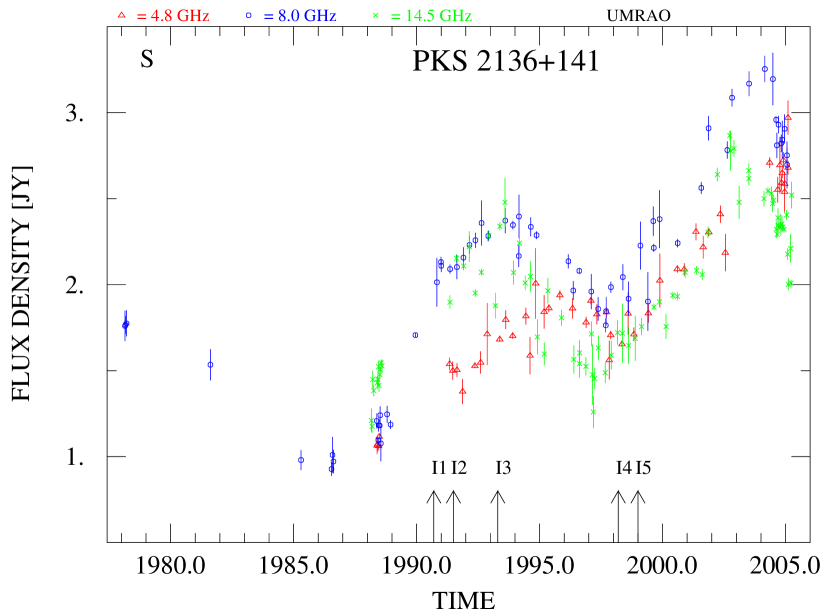
Figure 1.— Weekly averages of total flux density for PKS 2136+141 (OX 161) from UMRAO centimetre band monitoring. Observations at 14.5, 8.0 and 4.8 GHz are denoted by (green) crosses, (blue) circles and (red) triangles, respectively. Extrapolated ejection epochs of VLBI components are marked with arrows. Component I6 is left out from the figure because it is seen only at the last epoch of the VLBA 2 cm Survey monitoring data, and therefore, we cannot accurately determine its ejection epoch. The ejection of I6 must have occured at sometime between the ejection of I5 and April 2004, when it is first observed. See the on-line edition for a color version of the figure.

Originally, Tornikoski et al. (2001) identified PKS 2136+141 (catalog ) as a candidate gigahertz-peaked spectrum source (GPS) having a slightly inverted spectrum up to 8-10 GHz in the intermediate-to-quiescent state and a clearly inverted spectrum ($\alpha\geq+0.5$) during outbursts. The high turnover frequency reported in Tornikoski et al. (2001) even puts PKS 2136+141 (catalog ) in the class of high frequency peakers (HFP). Although Torniainen et al. (2005) have recently classified the source as a flat spectrum radio source having a convex spectrum only during outbursts, the simultaneous continuum spectra from RATAN-600 (Kovalev et al., 1999, S. Trushkin, private communication) do show a convex shape also in the intermediate-to-quiescent state, albeit with a little lower peak frequency. The source is variable at radio frequencies showing a factor of $\sim 3$ variations in cm-wavelength flux curves with characteristic time scale of $\sim 5-6$ years (see Figure 1). The last strong outburst started around 1998 and peaked in late 2002 and in early 2004 at 14.5 and 8 GHz, respectively. This indicates that both, our multi-frequency observations in 2001 and 15 GHz VLBA monitoring during 1995-2004, caught the source during a major flare.

The paper is organized as follows: the multi-frequency VLBA data demonstrating the 210$\arcdeg$ bend of the jet, together with a space-VLBI observation from the HALCA satellite, are presented in § 2. In § 3, we present a kinematic analysis, derived from over eight years of the VLBA 2 cm Survey monitoring data at 15 GHz, indicating non-ballistic motion of the jet components. Also, changes in $\beta_{\mathrm{app}}$ and in the apparent half-opening angle of the jet are investigated. In § 4, possible reasons for observed bending are discussed and a helical streaming model explaining the observed structure is presented. Conclusions are summarized in § 5. Throughout the paper we use a contemporary cosmology with $H_{0}$ = 71 km s^-1 Mpc^-1, $\Omega_{M}$ = 0.27 and $\Omega_{\Lambda}$ = 0.73. For this cosmology and a redshift of 2.427, an angular distance of 1 mas transforms to 8.2 pc and a proper motion of 0.1 mas yr^-1 to an apparent speed of $9.2\,c$. We choose the positive spectral index convention, $S_{\nu}\propto\nu^{+\alpha}$.

Table 1Parameters of the Images for Figures  2 and  3

Frequency	$\Theta_{b,\textrm{\scriptsize{maj}}}$	$\Theta_{b,\textrm{\scriptsize{min}}}$	P.A.	rms noise	Peak Intensity	Contour $c_{0}$
(GHz)	(mas)	(mas)	(deg)	(mJy beam-1)	(mJy beam-1)	(mJy beam-1)
2	6.12	3.02	-11.7	0.4	1153	1.2
5	3.37	1.70	-12.5	0.2	1811	0.6
5	0.75	0.59	-26.6	8.3	708	24.9
8	1.98	1.01	-7.8	0.2	1890	0.6
15	0.90	0.50	-7.5	0.5	1429	1.5
22	0.63	0.36	-7.9	1.2	1153	3.6
43	0.43	0.18	-16.1	1.5	512	4.5

2. MULTI-FREQUENCY OBSERVATIONS

On May 2001 we made multi-frequency polarimetric VLBI observations of four HFP quasars, including PKS 2136+141 (catalog ), using the VLBA. Observations were split into a high frequency part (15, 22 and 43 GHz), which was observed on the 12th of May, and into a low frequency part (2.3, 5 and 8.4 GHz) observed on the 14th of May. Dual polarization was recorded at all frequencies.

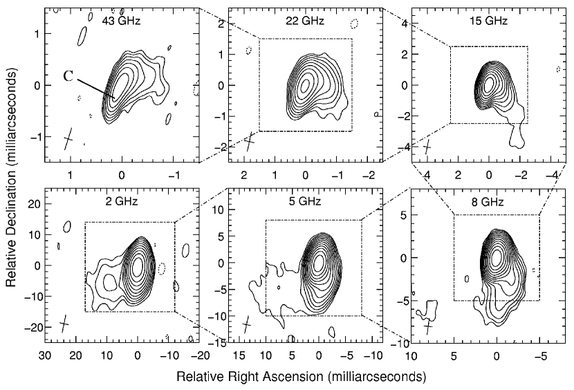
Figure 2.— Total intensity VLBA observations of PKS 2136+141 from May 2001. The compiled figure shows images of the source at all six observed frequencies (2.3, 5, 8.4, 15, 22, and 43 GHz). The letter “C” in the top left panel marks the location of the core. The size and orientation of the beam is shown in the lower left corner of each image. Peak intensities and contour levels are given in Table 1.

2.1. Reduction of the VLBA Data

The data were correlated with the VLBA correlator in Socorro and were postprocessed in Tuorla Observatory using the NRAO’s Astronomical Image Processing System, AIPS, (Bridle & Greisen, 1994; Greisen, 1988) and the Caltech difmap package (Shepherd, 1997). Standard methods for VLBI data reduction and imaging were used. An a priori amplitude calibration was performed using measured system temperatures and gain curves. For the high frequency data (15–43 GHz), a correction for atmospheric opacity was applied. After the removal of a parallactic angle phase, a single-band delay and phase off-sets were calculated manually by fringe fitting a short scan of data of a bright source. We did manual phase calibration instead of using pulse-cal tones, because there were unexpected jumps in the phases of the pulse-cal tones during the observations. Global fringe fitting was performed, and the delay difference between right- and left-hand systems was removed (for the purpose of future polarization studies). Bandpass corrections were determined and applied before averaging across the channels, after which the data were imported into difmap.

In difmap the data were first phase self-calibrated using a point source model and then averaged in time. We performed data editing in a station-based manner and ran several iterations of clean and phase self-calibration in Stokes I. After a reasonable fit to the closure phases was obtained, we also performed amplitude self-calibration, first with a solution interval corresponding to the whole observation length. Solution interval was gradually shortened as the model improved by further cleaning. Final images were produced with the Perl library FITSPlot.

We have checked the absolute flux calibration by comparing the extrapolated zero baseline flux density of our compact calibrator source 1749+096 (catalog ) at 5, 8.4, and 15 GHz to the single-dish measurements made at University of Michigan Radio Astronomy Observatory (UMRAO), and at 22 and 43 GHz to the fluxes from Metsähovi Radio Observatory’s quasar monitoring program at 22 and 37 GHz, respectively (Teräsranta et al., 2004). The flux densities agree to 5% at 8.4, 15, 22 and 37/43 GHz, and to 8% at 5 GHz, which is better than the expected nominal accuracy of 10% for the a priori amplitude calibration. Being unable to make a flux check for the 2.3 GHz data, we conservatively estimate it to have an absolute flux calibration accurate to 10%.

In order to estimate the parameters of the emission regions in the jet, we model-fitted to the self-calibrated (u,v) data in difmap. The data were fitted with a combination of elliptical and circular Gaussian components, and we sought to obtain the best possible fit to the visibilities and to the closure phases. Several starting points were tried in order to avoid a local minimum fit. We note that since the source structure is complex, the models are not unique, but rather show one consistent parameterization of the data. Based on the experiences in error estimation reported by several groups, we assume uncertainties in component flux $\sim 5$%, in position $\sim 1/5$ of the beam size (or of the component size if it is larger than the beam), and in size $\sim 10$% (see e.g. Jorstad et al. (2005) and Savolainen et al. (2006) for recent discussions on the model fitting errors). Although Jorstad et al. (2005) use larger positional uncertainties for weak knots having flux densities below 50 mJy, we use $\sim 1/5$ of the beam size (or of the component size) also for these components. Bigger uncertainties would result in such a large ratio of the individual errors to the scatter of the component positions (about the best-fit polynomial describing the component motion) that it would be statistically unlikely (see § 3.1.2).

A detailed description of the polarization data reduction and imaging in Stokes Q and U together with polarization images will appear in T. Savolainen et al. (in preparation).

2.2. Reduction of the HALCA data

Figure 3.— 5 GHz space-VLBI image of PKS 2136+141 observed on 1998 May 28. Beam size, peak intensity and contour levels are given in Table 1.

The 5 GHz space-VLBI observations of PKS 2136+141 (catalog ) were carried out as a part of the VSOP survey program (Hirabayashi, 2000, R. Dodson et al. in preparation) on 1998 May 28. In addition to the HALCA satellite, the array consisted of Arecibo, Haartebesthoek, and the Green Bank (140 ft) telescopes. The data were correlated using the Penticton correlator and reduced using the same standard methods as for the ground based images. Due to the small aperture of the HALCA satellite, its weight was increased to 10 to persuade the fitting algorithm to take better account of the long space baselines.

The dynamic range of the resulting image is rather small. This is due to a component that had a strong effect only to a single baseline between Arecibo and Green Bank. Because the (u,v) coverage is very limited, all attempts to model this component diverged. By manually changing the model to follow the visibility amplitudes in this scan, we estimate that the position of this component is about 7 mas at a PA of 100^∘. Because this component could not be formally included in the model, the residuals are rather strong and thus the imaging noise is high.

2.3. Source Structure from the Multi-Frequency Data

Figure 2 displays images of PKS 2136+141 (catalog ) at all six observed frequencies. In the images at 15, 22 and 43 GHz, uniformly weighted (u,v)-grids are employed in order to achieve the best possible resolution, whereas normal weighting is used in the low frequency maps to highlight diffuse, low surface brightness emission. The restoring beam sizes, peak intensities, off-source rms noise, and contour levels of the images are given in Table 1.

The multi-frequency images strikingly reveal a jet which gradually bends $210\arcdeg$ with its structural P.A. turning clockwise from -27$\arcdeg$ at 43 GHz to +123$\arcdeg$ at 2.3 GHz. We identify the bright and the most compact model component lying in the south-east end of the jet in the 15–43 GHz images as the core, and mark it with a letter “C”. The identification is confirmed by a self-absorbed spectrum of the component, as will be shown later. Between about 0.4-1.0 mas from the core, the jet turns over $90\arcdeg$, which is visible in 15–43 GHz images, and in the image taken at 8.4 GHz, the jet direction continues to turn clockwise $\sim 50\arcdeg$ at about 3.5 mas from the core. There is also evident bending in the 5 and 8.4 GHz images: a curve of $\sim 70\arcdeg$ takes place at about 6 mas south of the core. It is not totally clear, whether the trajectory of the jet is composed of a few distinct bends or whether it is a continuous helix. However, the gradual clockwise turn and the apparent spiral-like appearance of the jet in the multi-frequency images are highly reminiscent of a helical trajectory. Also, it seems unlikely that the jet goes through at least three consecutive deflections with all of them having the same sense of rotation in the plane of the sky.

The 5 GHz space-VLBI image of PKS 2136+141 (catalog ) from 1998 May 28, i.e. three years before the multi-frequency VLBA observations, shows a rather compact core-jet structure with an extended emission to north-west (Figure 3). The jet takes then a sharp $90\arcdeg$ bend to south-west within about 1 mas from the core. This 5 GHz image shows a very similar curved structure near the core that can be seen in our ground-based 15 GHz image with matching resolution. Hence, the observed large-angle bending between the images taken at different frequencies cannot be attributed to frequency dependent opacity effects.

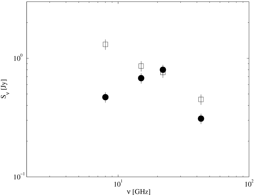
Figure 4.— Spectra of the core (filled circles) and the component I5 (open squares) at 8–43 GHz on May 2001.

PKS 2136+141 (catalog ) is rather compact at all frequencies with a maximum jet extent of approximately 15 mas corresponding to $\sim 120$ pc at the source distance. The two brightest model components are the core and a newly ejected component I5 (see §3 for component identifications), which is located at $\sim 0.25$ mas from the core – near the beginning of the first strong bend in the jet. Figure 4 shows the 8–43 GHz spectra of these two components. At 2.3 and 5 GHz the angular resolution is too poor to separate the core from I5, and hence, corresponding flux values are omitted in the figure. The core has a synchrotron peak frequency of $\sim 20$ GHz, while the newly ejected component I5 shows an optically thin synchrotron spectrum with a spectral index $\alpha=-0.6$ and a peak frequency below 8 GHz. The component I5 is brighter than the core at every frequency except at 22 GHz, where almost equal flux densities are measured. An optically thick spectrum of the core at frequencies below 22 GHz indicates that I5 is brighter than the core also at 2.3 and 5 GHz, although the spectra cannot be measured at those frequencies. The self-absorbed spectrum shown in Figure 4 confirms that we have correctly identified the core.

3. VLBA 2 CM SURVEY AND MOJAVE DATA

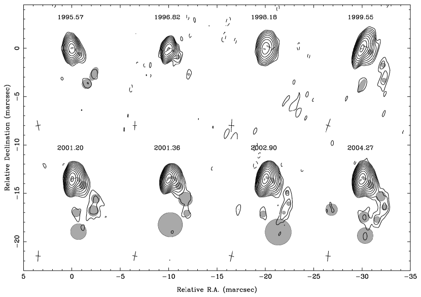
Figure 5.— VLBA images of PKS 2136+141 at 15 GHz. The figure includes observations from the VLBA 2 cm Survey, from the MOJAVE Survey and a 15 GHz image from our multi-frequency data set observed in 2001.36. In all images, a uniformly weighted (u,v)-grid is used. The Gaussian components fitted to the visibility data are shown as ellipses overlaid each image. The size and orientation of the beam is shown in the lower left corner of each image. Peak intensities and contour levels are given in Table 2.

Table 2Parameters of the Images for Figure 5

Epoch	$\Theta_{b,\textrm{\scriptsize{maj}}}$	$\Theta_{b,\textrm{\scriptsize{min}}}$	P.A.	rms noise	Peak Intensity	Contour $c_{0}$
(yr)	(mas)	(mas)	(deg)	(mJy beam-1)	(mJy beam-1)	(mJy beam-1)
1995.57	1.01	0.53	11.5	0.9	1254	2.7
1996.82	0.92	0.41	-1.6	0.8	633	2.4
1998.18	1.31	0.61	-3.4	1.4	929	4.2
1999.55	1.45	0.49	-19.6	0.7	1429	2.1
2001.20	1.14	0.52	-3.1	0.4	1153	1.2
2001.36	0.90	0.50	-7.5	0.5	1429	1.5
2002.90	1.15	0.55	-12.9	0.4	2120	1.2
2004.27	1.09	0.54	-5.7	0.3	1745	0.9

Seven observations of PKS 2136+141 (catalog ) have been performed as part of the VLBA 2 cm Survey (Kellermann et al., 1998; Zensus et al., 2002) between 1995 and 2004 of which the last one (epoch 2004.27) was part of the follow-up program MOJAVE (Lister & Homan, 2005). Details on the survey observing strategy, the observing details and the data reduction can be found in the mentioned publications.

clean VLBI images of PKS 2136+141 (catalog ) have been produced by applying standard self-calibration procedures with difmap for all seven epochs. The calibrated visibility data were fitted in the (u,v) domain with two-dimensional elliptical Gaussian components (see Figure 5). Because of the complicated source structure, no adequate model representation of the source could be established with a smaller number of components than shown in Figure 5. Moreover, the components are found to be located close-by along the curved inner part of the jet, in many cases separated from each other by considerably less than one beam size. Special care had to be taken to find a model of this complicated structure in a consistent way for all epochs.

3.1. Source Kinematics

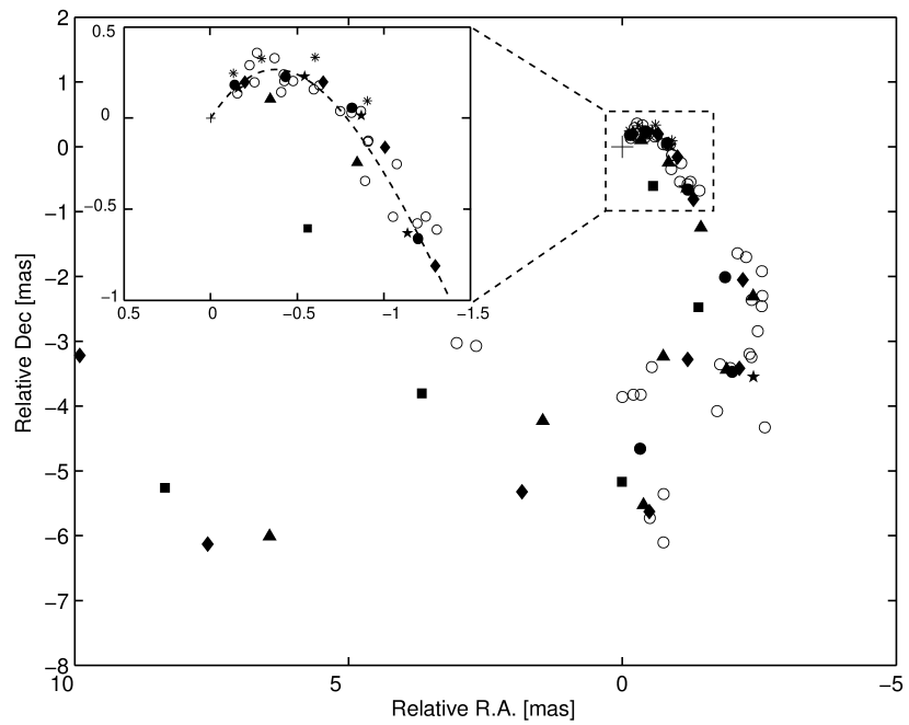
Figure 6.— Model-fit component locations. Open circles are model components from the VLBA 2 cm Survey monitoring and filled symbols show the multi-frequency data: squares – 2.3 GHz, triangles – 5 GHz, diamonds – 8.4 GHz, circles – 15 GHz, stars – 22 GHz, and asterisks – 43 GHz. The position of the core is marked with a cross. The inset is an enlarged plot of the innermost 2 x 1.5 mas and it also displays an approximate ridge line of the jet.

A crucial question raised by the apparent helical shape of the jet in Figure 2 is, whether it represents streaming motion or whether the helix is due to a precessing jet nozzle ejecting material that moves along ballistic trajectories. We have plotted positions of all model-fit components from the multi-frequency data and from eight years of the VLBA 2 cm Survey monitoring data into Figure 6. The open circles, which correspond to the multiepoch data from the VLBA 2 cm Survey, form a dense and strongly curved region near the base of the jet, a $\sim 2$ mas long continuous and slightly curved section 3.5 mas south-west of the core, and a few small isolated groups. This subtle finding alone, without invoking any component identification scenarios, demonstrates that ballistic-motion models are unlikely to yield a meaningful representation of the jet kinematics in PKS 2136+141 (catalog ). Brightening at certain points of the jet can be either due to an increased Doppler factor (if a section of the jet bends towards our line of sight), or due to an impulsive particle acceleration in a standing shock wave (e.g. forming in the bend). There seems to be a zone of avoidance in the 15 GHz data between the base of the jet and the large western group, further supporting this idea.

We have analyzed the jet kinematics using source models derived from the VLBA 2 cm Survey monitoring data. In a complicated source like PKS 2136+141 (catalog ) it is often difficult to identify components across epochs with confidence. We have based our identifications on the most consistent trajectories, and on the flux density evolution of the components. We restrict our analysis to a full kinematical model for the inner 2 mas of the jet, since beyond that distance a fully self-consistent model could not be established due to the lower surface brightness and high complexity in the outer region.

3.1.1 Component Trajectories and Flux Evolution

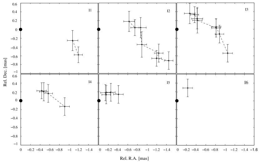
Figure 7.— Trajectories of components I1–I6. Positions are measured relative to the core, which is placed into the origin in each panel (filled circle). The errorbars correspond to $1/5$ of the beam size.

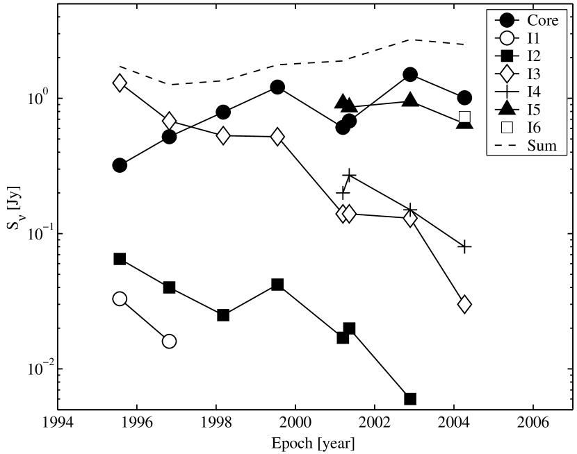
Figure 8.— Flux densities of the identified components from the VLBA 2 cm Survey monitoring.

Figure 7 shows the trajectories of the six compact components (I1-I6) which we have identified in the inner 2 mas of the jet. The components travel towards south-west and their trajectories do not extrapolate back to the core implying that the components travel along a curved path, and the jet is non-ballistic. The components fade below the detection limit within $\sim 1.6$ mas from the core, and we cannot follow them further.

We present the flux density evolution of the six inner-jet components in Figure 8. The overall picture is that the fluxes decrease as the components move forward along their path. They reach about 5–15 mJy by the time they have traveled to a distance of $\sim 1.5$ mas from the core, after which they are not seen anymore. The knot I3 is the brightest component of the source at the first two epochs, and its flux density evolution matches well with the strong 1993 flare visible in the 14.5 GHz UMRAO flux density curve (see Figure 1). The ejections of the components I1 and I2 (see Table 4) take place during the rising phase of the 1993 outburst, and the component I3 is ejected just before the outburst reaches its maximum.

The core has a steadily rising flux density until 2001.20, when the flux suddenly drops and two new components, I4 and I5, appear. At the next two epochs, the core flux increases again and at the last epoch (2004.27) there is a drop accompanied by an appearance of a new component, I6. The brightening of the core during our monitoring and ejections of components I4, I5, and I6 correspond to a strong total flux density flare peaking in late 2002 at 14.5 GHz (again, see the total flux density curve in Figure 1).

The above-mentioned flux density evolution of the components is self-consistent and it is well in accordance with the general behavior of flat-spectrum radio quasars during strong total flux density flares (Savolainen et al., 2002), i.e. a compact VLBI core is mostly responsible for the rising part of the observed flares in single-dish flux curves, and a new component appears into the jet during or after the flare peaks accompanied by a simultaneous decrease in the core flux density. The fact that the overall flux density evolution of the identified components in PKS 2136+141 (catalog ) seems to obey the common behavior identified for a number of other sources supports our kinematical model. An intriguing detail is the consecutive ejection of, not one, but three new components in connection with a single, strong total flux density flare. This may indicate that there is some substructure in the flares, i.e. the outbursts in 1993 and 2002 could be composed of smaller flares. On the other hand, it could also mean that a single strong event in the total flux density curve is able to produce complicated structural changes in the jet, e.g. forward and reverse shocks could both be visible, or there could be trailing shocks forming in the wake of the main perturbance as theoretically predicted by Agudo et al. (2001) and recently observed in several objects, most prominently in 3C 111 (catalog ) (Jorstad et al., 2005; Kadler, 2005, Kadler et al. in preparation) and in 3C 120 (catalog ) (Gómez et al., 2001).

3.1.2 Apparent Velocities and Acceleration

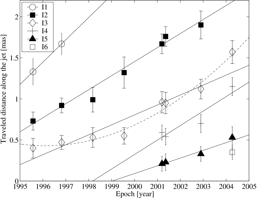
Figure 9.— Component motion along the jet ridge line. The symbols for different component are: open circles – I1, filled squares – I2, open diamonds – I3, crosses – I4, filled triangles – I5, and an open square – I6. The solid lines represent linear fits to the data, and the dashed line represents a second-order fit.

Identification of the model-fit components across the epochs allows us to estimate the velocities of the components and to search for possible acceleration or deceleration. Since the components follow a highly curved path, we choose to measure the distance traveled along the jet by using an average ridge line, which is shown by the dashed line in Figure 6. The ridge line is determined by fitting a smooth function to the positions of model components within the inner 2 mas of the jet.

Figure 9 displays the motion of the components along the jet. To measure the component velocities and to estimate the ejection epochs, we have made standard linear least-squares-fits to the motions:

$$l(t_{i}) = a_{0}+a_{1}(t_{i}-t_{\mathrm{mid}}),$$ (1)

where $l$ is the traveled distance along the jet, $t_{i}$ is the epoch of observation $(i=1,\ldots,N)$ and $t_{\mathrm{mid}}=(t_{1}+t_{N})/2$. In order to search for a possible acceleration or a deceleration, we have also fitted the components I2 and I3, which are observed over most epochs, by second-order polynomials:

$$l(t_{i}) = a_{0}+a_{1}(t_{i}-t_{\mathrm{mid}})+a_{2}(t_{i}-t_{\mathrm{mid}})^{2}.$$ (2)

To assess the goodness of the fits, we have calculated a relative $\chi^{2}$ value for each fit. The $\chi^{2}$ values are relative, not absolute, since we do not strictly know the real $1\sigma$ measurement errors of the component positions but have instead used $1/5$ of the beam size projected onto the ridge line. Although the “$1/5$ of the beam size” estimate for the errors is rather well-justified in the literature, it is likely to be conservative. Thus the tabulated values of $\chi^{2}$ distribution do not provide a good statistical test of the goodness of the fits in our case. However, we assume that the beam sizes give a good estimate of the relative errors between the epochs, and hence, only one scaling factor (which is close to unity) for the positional errors (and for the $\chi^{2}$ values) remains unknown. With this assumption, the relative $\chi^{2}$ values can be used to compare the goodness of the fits against each other. The parameters of the fitted polynomials are given in Table 3 together with relative reduced $\chi^{2}$ values and the number of the degrees of freedom, $\nu$, for each fit.

We have gathered the average angular velocities along the jet, $\langle\mu\rangle=a_{1}$, the average apparent speeds, $\langle\beta_{\mathrm{app}}\rangle$, and the epochs of zero separation, $T_{0}$, for each component in Table 4. For the second-order fits, also the angular acceleration along the jet, $\dot{\mu}=2a_{2}$, is reported. The proper motions range from 0.09 to 0.27 mas yr^-1, corresponding to the apparent superluminal velocities of $8.7-25.1\,c$.

Table 3Best-Fit Polynomials for the Motion of Components I1–I5

Comp.	$k$	$a_{0}$	$a_{1}$	$a_{2}$	$\chi^{2}/\nu$	$\nu$
I1	1	$1.50\pm 0.10$	$0.27\pm 0.17$	$\cdots$	$\cdots$	0
I2	1	$1.32\pm 0.05$	$0.17\pm 0.02$	$\cdots$	0.34	5
	2	$1.29\pm 0.08$	$0.17\pm 0.02$	$0.01\pm 0.01$	0.37	4
I3	1	$0.80\pm 0.04$	$0.12\pm 0.02$	$\cdots$	1.50	6
	2	$0.68\pm 0.06$	$0.13\pm 0.02$	$0.02\pm 0.01$	0.43	5
I4	1	$0.81\pm 0.05$	$0.18\pm 0.04$	$\cdots$	1.19	2
I5	1	$0.35\pm 0.06$	$0.09\pm 0.04$	$\cdots$	0.12	2

While the component I2 is well-fitted by a straight line, the linear proper motion model does not seem to adequately represent the motion of the component I3 as can be seen from Figure 9. On the other hand, a second-order polynomial gives an acceptable fit to I3, and its relative $\chi^{2}$ value divided by the number of the degrees of freedom is by a factor of 3.5 smaller than the value for the first-order polynomial. However, the small number of data points and the uncertainty about the real $(1\sigma)$ errors in the component positions makes it difficult to give a statistical significance of the deviation from the constant speed model. We have used two approaches to assess the significance. The most robust and the most straightforward test is to use a statistic $F_{\nu_{1},\nu_{2}}\equiv(\chi^{2}_{1}/\nu_{1})/(\chi^{2}_{2}/\nu_{2})$, which has an $F$-distribution with $(\nu_{1},\nu_{2})$ degrees of freedom, and which is independent of the unknown scaling factor in the positional errors. This statistics can be used to test whether the squared residuals of the linear model are significantly larger than those of the accelerating model. As already mentioned, for the first and the second-order polynomials in the case of I3, $F_{6,5}=3.5$, which implies a difference in the residuals only at the confidence level of $\alpha=0.10$; i.e. according to the $F$-test, the statistical significance of the difference in the residuals is only marginal. Another approach to this problem is to try to estimate the real $1\sigma$ uncertainties of the component positions by applying a method described by Homan et al. (2001). They estimated the uncertainties of the fitted parameters of their proper motion models by using the variance about the best-fit model, and as a by-product they obtained an upper bound estimate of the component position uncertainty. Since the relative $\chi^{2}$ values divided by the degrees of freedom are significantly less than unity for components I2 and I5 (the situation of component I4 is discussed later), we suspect that the real $1\sigma$ positional uncertainties are in fact smaller than $1/5$ of the beam size. If the beam sizes give a good estimate of the relative errors between the epochs, we can try to estimate the uniform scaling factor for the positional uncertainties by requiring that $\chi^{2}\simeq\nu$ for the linear proper motion models of I2, I4, and I5. The sum $\Sigma_{i}(\chi_{i}^{2}/k^{2}-\nu_{i})^{2},\,(i=\mathrm{I2,I4,I5})$ is minimized for the positional error scaling factor $k=0.77$; i.e. the $1\sigma$ positional uncertainties are $0.77\times 1/5$ of the beam size $\approx 0.08-0.15$ mas. If these $(1\sigma)$ uncertainties are assumed, the linear fit to the motion of component I3 has $\chi^{2}=15.2$ with 6 degrees of freedom, implying that the speed of I3 is not constant at the significance level of $\alpha=0.025$.

Table 4Proper Motions of Model-Fit Components

Comp.	$k$	$\dot{\mu}$	$\langle\mu\rangle$	$\langle\beta_{\mathrm{app}}\rangle$	$T_{0}$
		(mas yr-2)	(mas yr-1)	$(c)$	(yr)
I1	1	$\cdots$	$0.27\pm 0.17$	$25.1\pm 15.2$	$1990.7\pm 3.0$
I2	1	$\cdots$	$0.17\pm 0.02$	$15.8\pm 1.8$	$1991.5\pm 0.6$
	2	$0.01\pm 0.02$	$0.17\pm 0.02$	$16.0\pm 1.8$	$\cdots$
I3	1	$\cdots$	$0.12\pm 0.02$	$11.2\pm 1.9$	$1993.3\pm 0.6$
	2	$0.03\pm 0.01$	$0.13\pm 0.02$	$11.7\pm 1.4$	$\cdots$
I4	1	$\cdots$	$0.18\pm 0.04$	$16.2\pm 3.9$	$1998.2\pm 0.8$
I5	1	$\cdots$	$0.09\pm 0.04$	$8.7\pm 4.1$	$1999.0\pm 1.2$

Note. — See text for the definitions of $\dot{\mu}$, $\langle\mu\rangle$, $\langle\beta_{\mathrm{app}}\rangle$, and $T_{0}$.

Component I4 seems to show motion that indicates acceleration similar to I3, but since there are only four data points for I4, we have not fitted it with a second-order polynomial, which would leave only one degree of freedom for the fit. By looking at Figure 9, one can see that I4 should have been present in the jet already at the epoch 1999.55, but it cannot be unambiguously inserted into the source model; i.e. adding one more component in the model does not improve the fit, but rather makes the final fit highly dependent on the chosen initial model parameters. One possible explanation is that the proper motion for I4 is faster than indicated by the best-fit line in Figure 9, and it is not actually present in the jet in 1999.55. A second possibility is that I4 is a trailing shock released in the wake of the primary superluminal component I3 instead of being ejected from the core (Agudo et al., 2001; Gómez et al., 2001). This alternative is not a very plausible one, since according to Agudo et al. (2001) trailing shocks should have a significantly slower speed than the main perturbance. A third possible explanation for the non-detection of I4 in 1999.55 is that either I4 and the core or I4 and I3 are so close to one another in 1999.55 that they do not appear as separate components in our data.

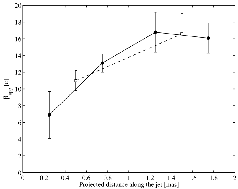
Figure 10.— Apparent velocity of the components as a function of projected distance along the jet. The figure shows two different bin widths: open squares – a bin width of 1.0 mas, and filled circles – a bin width of 0.5 mas.

As discussed above, we cannot firmly establish that component I3 accelerates along the jet ridge line, although it seems probable. However, also the other components (apart from I4, which itself might show acceleration) appear to be systematically faster, the farther away from the core they lie. We have averaged the velocities of the individual components over traveled distance bins of 1.0 and 0.5 mas. In averaging, we have taken into account the standard errors given in Table 4 and the fact that for a given component in a given bin, the weight has to be decreased, if the first or the last observation of the component falls into that bin. This is because naturally we do not have any knowledge about the component speed before or after our observations. For component I3 we have used the quadratic fit instead of the linear, since it much better describes the data. The binned velocities are presented in Figure 10, which suggests that there is acceleration along the jet ridge line. When the data is divided in four bins, the first bin (0–0.5 mas) has an average component velocity of $\approx 7\pm 3\,c$, while the rest of the bins (0.5–2.0 mas) have significantly higher velocities, the maximum being $\approx 17\pm 3\,c$ for the bin covering 1.0–1.5 mas. For the division in two bins, the change is from $\approx 11\pm 1\,c$ in the first bin to $\approx 17\pm 3\,c$ in the second. The acceleration takes place in the first strong bend of the jet, which seems very natural since the apparent velocity depends on the angle between the local direction of the jet flow and our line of sight. The acceleration in Figure 10 can alternatively be explained with the component speed changing as a function of ejection epoch – a new component (I5) being slower than the old ones (I1–I2). This, however, does not explain the likely acceleration of I3. Thus we regard the change in $\beta_{\mathrm{app}}$ along the jet ridge line as probable although more data is needed for conclusive evidence.

Kellermann et al. (2004) parameterized the $1995-2001$ VLBA 2 cm Survey data of PKS 2136+141 (catalog ) by fitting Gaussian components to the brightest features of each epoch in the image plane and derived a speed of $\beta_{\mathrm{app}}=1.8\pm 1.4$, which is much lower than our estimates. Basically, their approach traces the component I3 over the time when its proper motion was slow (see Figure 9), and due to the curved path of I3, the speed measured from the changes in its radial distance from the core is also lower than its true angular velocity. A linear least-squares-fit to the radial distances of I3 in our data over the epochs $1995-2001$ yields $\beta_{\mathrm{app}}=2.6$, which agrees with the speed given in Kellermann et al. (2004) within the errors.

3.2. Apparent Half-Opening Angles and Jet Inclination

The angle between the local jet direction and our line of sight affects also the apparent opening angle of the jet. Assuming that the jet has a conical structure and a filling factor of unity, we have estimated the local value of the apparent half-opening angle for component $i$ as $\Psi^{\mathrm{app}}_{i}=\tan^{-1}(d_{i}/l_{i})$, where $l_{i}$ is the distance of the component $i$ from the core measured along the jet ridge line, and $d_{i}=a_{i}/2+\Delta r_{i}$, with $a_{i}$ being the size of the elliptical component projected on the line perpendicular to the jet and $\Delta r_{i}$ being the normal distance of the component from the jet ridge line.

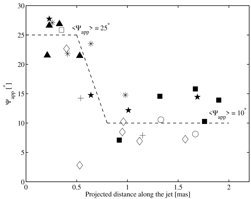
Figure 11.— Apparent half-opening angle $\Psi_{\mathrm{app}}$ of the components as a function of projected distance along the jet. The symbols for components I1-I6 are the same as used in Figs. 6 and 7. Stars correspond to components of the 22 GHz data and asterisks are for the 43 GHz components. The dashed line shows the average $\Psi_{\mathrm{app}}$ in two regions: 1) the innermost 0.5 mas, and 2) between 0.8–2.0 mas.

Figure 11 shows the apparent half-opening angle for components I1-I6 from 15 GHz data and for unnamed components from 22 and 43 GHz data as a function of traveled distance along the ridge line. The components with zero axial ratio have been excluded from the figure. Naturally, $\Psi_{\mathrm{app}}$ is very uncertain for a single component, but Figure 11 clearly shows that there is a change in the average $\Psi_{\mathrm{app}}$ between the first $\sim 0.5$ mas and $0.8-2.0$ mas, and the change seems to correspond to the first large bend in the jet. Within the first 0.5 mas, the average apparent half-opening angle is $\sim 25\arcdeg$ and further down the jet it decreases to $\sim 10\arcdeg$. A natural explanation for this effect is that the viewing angle $\theta$ increases in the first apparent bend, since $\Psi_{\mathrm{app}}\approx\Psi_{\mathrm{int}}/\sin\theta$ if $\theta$ and the intrinsic half-opening angle $\Psi_{\mathrm{int}}$ are both small. There is a caveat, though. Namely, the large value of $\Psi_{\mathrm{app}}$ near the core could be due to a resolution effect: if the positional uncertainties for the components near the core were $\sim 1/5$ of the beam size, $\Delta r$ of these components could be $\approx 0.1-0.2$ mas at 15 GHz merely due to the scatter, and this would result in $\langle\Psi_{\mathrm{app}}\rangle=25\arcdeg$. However, there are two reasons, why we think the observed change in $\Psi_{\mathrm{app}}$ is a true effect and due to a changing $\theta$. First, the model-fit components from 22 and 43 GHz data show similar values for $\Psi_{\mathrm{app}}$ near the core as the components from 15 GHz data, although they have a factor of 1.5–2 smaller positional errors. Secondly, the components near the core are bright, having fluxes comparable to the core, which makes their positional uncertainties smaller than the adopted $\sim 1/5$ of the beam size (see also the previous section for a discussion about the positional uncertainties). According to Jorstad et al. (2005) bright (flux of the knot $>100$ rms noise level) and compact (size $<0.1$ mas) features in the jet have positional uncertainties $\sim 0.01$ mas at 7 mm. Thus we regard the observed change in $\Psi_{\mathrm{app}}$ as a genuine effect.

The $\beta_{\mathrm{app}}$ of the jet seems to increase after $\sim 0.5$ mas from the core (see Figure 10) while the $\Psi_{\mathrm{app}}$ decreases. This can be understood, if the angle between local jet direction and our line of sight within the first $\sim 0.5$ mas is smaller than the angle $\theta_{SL}=\sin^{-1}(1/\Gamma)$, which maximizes $\beta_{\mathrm{app}}$. After 0.5 mas $\theta$ increases towards the maximal superluminal angle increasing $\beta_{\mathrm{app}}$ and decreasing $\Psi_{\mathrm{app}}$. Assuming that the largest velocity in Figure 10, $\beta_{\mathrm{app}}\approx 17\,c$, is close to the maximum apparent velocity (we do not consider the velocity of I1, 25.1 $c$, very reliable since it is based on only two data points, and hence, we do not use it in our estimation of the maximum $\beta_{\mathrm{app}}$), we can estimate that the jet Lorentz factor $\Gamma\sim 20$. Now, if we assume a constant Lorentz factor $\Gamma=20$, we can fit for the values of the viewing angle and the intrinsic jet half-opening angle giving the observed superluminal speeds and half-opening angles before and after the bend. For $\langle\beta_{\mathrm{app}}\rangle\approx 7\,c$, $\langle\Psi_{\mathrm{app}}\rangle\approx 25\arcdeg$ within the first 0.5 mas from the core and $\langle\beta_{\mathrm{app}}\rangle\approx 17\,c$, $\langle\Psi_{\mathrm{app}}\rangle\approx 10\arcdeg$ after the bend, we obtain the following best-fit values: $\theta(0-0.5\,\mathrm{mas})=0.6\arcdeg$, $\theta(1.0-2.0\,\mathrm{mas})=1.5\arcdeg$, and $\Psi_{\mathrm{int}}=0.26\arcdeg$. According to this result, the jet bends away from our line sight by $\approx 0.9\arcdeg$ after the first 0.5 mas from the core.

Naturally, it is possible that the components exhibit also real acceleration along the jet in addition to the apparent acceleration due to the projection effect. Unfortunately, the observations do not allow us to decide between these cases. Applying Occam’s razor, we consider a constant jet speed in the following discussion.

4. DISCUSSION

4.1. Possible Reasons for Bending

In this section we discuss the mechanisms capable of producing the curved structure of PKS 2136+141 (catalog ). In principle, there are several possible scenarios for the observed bending in relativistic jets, but we can rule out some of them in this particular case on the grounds of our analyzed data.

Projection effects play an important role in this case making the intrinsic bending angle much less than the observed one. If the angle between the jet and our line of sight is as small as the analysis in the previous section indicates, it is possible that, for example, within 0.5-1.0 mas from the core where the apparent bend is $\sim 90\arcdeg$, the intrinsic bending angle is only $\sim 1-2$ degrees. This implies that formation of internal shocks in the bend, and their possibly destructive effect to the collimation of the jet, is not of great concern here. Mendoza & Longair (2002) calculate an upper limit to the bending angle of a jet in order not to create a shock wave at the end of the curvature. Their result for relativistic jets is $\sim 50\arcdeg$, which leaves our estimated intrinsic bending angle for PKS 2136+141 (catalog ) well within the limits. Therefore, we do not consider internal shocks formed by bending to restrict the possible explanations for the curvature in this source.

One of the scenarios we can rule out, is a precessing jet where the components ejected at different times to different directions move ballistically, and form an apparently curved locus. Such models have been used to describe oscillating ’nozzles’ observed in some BL Lac sources (Stirling et al., 2003; Tateyama & Kingham, 2004). In the case of PKS 2136+141 (catalog ), we can reject the precessing ballistic jet hypothesis, since the individual components do not follow ballistic trajectories, but rather exhibit streaming motion along a curved path (see §3.1.1). However, precession of the jet inlet may still be behind the observed structure if it serves as an initial perturbation driving a helical Kelvin-Helmholtz normal mode (see §4.2).

Homan et al. (2002) explained the large misalignment between the pc and kpc scale jets of PKS 1510-089 (catalog ) with a scenario where the jet is bent after it departs the host galaxy, either by a density gradient in the transition region or by ram pressure due to the winds in the intracluster medium. In PKS 2136+141 (catalog ) the bending starts within 0.5 mas from the core, and because $\theta=0.6_{-0.3}^{+0.2}$ degrees for the inner part of the jet (the error range here refers to an uncertainty introduced by errors in $\langle\beta_{\mathrm{app}}\rangle$; see § 3.1.2 and 3.2), the corresponding deprojected distance is smaller than 0.8 kpc. The whole bending visible in Figure 2 takes place within about 15 mas from the core. Given the viewing angles estimated in § 3.2, it is fair to say that the deprojected length of the jet is – probably significantly – less than $\sim 12$ kpc, and the whole observed bending takes place within that distance from the core. There are no observations of the host galaxy of PKS 2136+141 (catalog ), but the deprojected lengths estimated above can be compared with typical scalelengths of the elliptical hosts of radio-loud quasars (RLQs), which are reported by several groups. In their near-infrared study, Taylor et al. (1996) found low-redshift $(z\sim 0.2)$ RLQ hosts to have very large half-light scalelengths $R_{\mathrm{1/2}}$; from 14.0 to 106.8 kpc with an average of $\sim 30$ kpc. Other studies have yielded smaller values: e.g. Floyd et al. (2004) used Hubble Space Telescope WFPC2 data to study hosts of 17 quasars at $z\sim 0.4$ finding $\langle R_{\mathrm{1/2}}\rangle=10.2\pm 1.8$ kpc for RLQs, and Kotilainen et al. (1998) reported $\langle R_{\mathrm{1/2}}\rangle=13\pm 7$ kpc for 12 flat spectrum radio quasars up to $z=1.0$ in their near-infrared study. In the framework of hierarchical models of galaxy formation, the hosts of quasars at high redshift are also expected to be more compact than their low-redshift counterparts. Falomo et al. (2005) have recently managed to resolve a quasar host at $z=2.555$ and they report an effective radius of $7.5\pm 3$ kpc. As the deprojected distance $\lesssim 0.8$ kpc indicates, the bending of the jet in PKS 2136+141 (catalog ) starts well within the host galaxy, and the typical scalelengths listed above suggest that most of the curved jet is located within the host, although it is possible that part of it lies in the outskirts of the host galaxy being susceptible to the density gradient in the transition region. However, the bending clearly starts inside the galaxy, and thus requires some other cause.

A collision inside the host galaxy, between the jet and a cloud of interstellar matter, can change the direction of the flow. For example, Homan et al. (2003) have found component C4 in 3C 279 (catalog ) to change its trajectory by $26\arcdeg$ in the plane of the sky, and they suggest this to be due to a collimation event resulting from an interaction of the component with the boundary between the outflow and the interstellar medium. However, the mere fact that the observed $\Delta$P.A. is larger than 180$\arcdeg$ in our case constrains the collision scenario since it excludes the situations where the jet is bent by a single deflection, e.g. from a single massive cloud. In principle, the observed structure may be due to several consecutive deflections from a number of clouds, but, as already mentioned in §2.3, this would require there to be at least three successive deflections having the same sense of rotation in the plane of the sky. This is unlikely, although not impossible. Future observations aimed at detecting emission from the jet beyond 20 mas will be very interesting, since they could tell whether the bending continues in the larger scale or not. If curvature with the same sense of rotation as within 15 mas is observed also in the larger scale, the scenario with multiple deflections from ISM clouds seems highly unlikely.

4.2. Helical Streaming Model

Relativistic jets are known to be Kelvin-Helmholtz unstable, and they can naturally develop helical distortions if an initial seed perturbation is present at the jet origin. The helical K-H fundamental mode is capable of displacing the entire jet and consequently producing large scale helical structures where the plasma streams along a curved path (Hardee, 1987). The initial perturbations can have a random spectrum, and be due to for example jet-cloud interaction, or they can originate from a periodic variation in the flow direction of the central engine (precession or orbital motion). These perturbations can trigger pinch, helical or higher order normal modes propagating down the jet, and the appearance of this structure depends on the original wave frequency and amplitude, as well as subsequent growth or damping of the modes. Since the individual components in PKS 2136+141 (catalog ) do not follow ballistic trajectories, but rather seem to stream along a helical path, we consider a helical K-H fundamental mode to be a possible explanation for the curious appearance of this source. For simplicity, in the following discussion we limit ourselves to a purely hydrodynamical case and do not consider the effect of magnetic fields for the growth of K-H modes, nor discuss the current-driven instabilities, which can produce helical patterns in Poynting-flux dominated jets (Nakamura & Meier, 2004).

The appearance of the jet in PKS 2136+141 (catalog ) already suggests some properties of the wave. The fact that components are observed to follow a nearly stationary helix implies that the wave frequency of the helical twist, $\omega$, is much below the “resonant” (or maximally unstable) frequency $\omega^{*}$, which corresponds to the frequency of the fastest growing helical wave (Hardee, 1987). Such a low frequency, long wavelength helical twist suggests that the wave is driven by a periodic perturbation at the jet base. If the central source induced white-noise-like perturbations, we would expect to see structures corresponding to the fastest growing frequency, i.e. $\omega^{*}$ (Hardee et al., 1994).

Figure 12.— Best-fit trajectory and component centroid positions at different frequencies for the model describing a low-frequency helical fundamental mode of Kelvin-Helmholtz instability.

If isothermal jet expansion without gradients in the jet speed or in the ratio of the jet and external medium sound speeds is assumed, the wave speed, $\beta_{w}$ (in units of $c$), in the low frequency limit remains constant as the jet expands (Hardee, 2003). Since the intrinsic wavelength, $\lambda$, for a given $\omega$ varies proportional to the the wave speed, it can be also assumed to remain constant along the jet (as long as $\omega\ll\omega^{*}$). Applying this assumption, we have fitted a simple helical twist to the observed positions of the VLBI components. The helical twist is specified in cylindrical coordinates with $z$ along the axis of helix, by an amplitude $A$ in the radial direction, and by a phase angle $\phi$ given by

$$\phi=2\pi h\int_{z_{1}}^{z}\frac{dz}{\lambda(z)}+\phi_{1},$$ (3)

where $h$ is the handedness of the helix ($-1$ for right-handed and $+1$ for left-handed), and $\phi_{1}=\phi(z_{1})$. With constant $\lambda$, the integral in equation (3) becomes trivial and $\phi\propto z$. The amplitude growth is assumed to be conical: $A=z\tan\psi_{c}$, where $\psi_{c}$ is the opening angle of the helix cone. To describe the orientation of the helix in the sky we use two angles: $i$ is the angle between the axis of the helix and our line of sight and $\chi$ is the position angle of the axis of the helix projected on the plane of the sky. There are altogether five parameters in the model since the handedness can be fixed to $h=+1$ by simply looking at the images.

Figure 13.— Viewing angle (top), Doppler factor (second from the top), apparent component speed (third from the top) and deprojected distance (bottom) for a jet with $\Gamma$ = 20 as a function of projected distance from the core along a helical model (see Figure 12). The two small vertical bars in the top panel show the viewing angle constraints obtained from the source kinematics and used in the modeling.

A computer program was written to fit the positions of the VLBI components with different models expected to explain the shape of the jet and the kinematics of individual components. In the program, the cumulative sum of perpendicular projected image-plane distances between a three-dimensional model and the component centroids from the VLBI observations was minimized using a differential evolution (Storn & Price, 1997) algorithm. This evolutionary algorithm was chosen because of its good performance with non-linear and multimodal problems. All the observed components (and all frequencies) were used in a single model-fit, because the components seem to follow a common path, i.e. the helical structure appears to persist for longer than the component propagation times. In addition to component positions on the plane of the sky, the model was constrained by the viewing angles determined in §3.2. The angle $\theta$ between the normal to the jet’s cross section and our line-of-sight was evaluated along the model, and it was required to be compatible with the viewing angles determined in §3.2. The following limits for $\theta$ were used: at 0.3 mas from the core $\theta$ is between $0.4-0.8\arcdeg$, and at 1.5 mas from the core $\theta$ is between $1.3-1.7\arcdeg$. If the model exceeded these limits, the cost function in the fitting algorithm was multiplied with a second-order function normalized to the width of the allowed range.

Table 5Best-fit Parameters of the Helical Streaming Model

Parameter	Symbol	Value
Initial helical wavelength [mas]	$\lambda_{1}$	776
Half-opening angle of the helix cone [deg]	$\psi_{c}$	1.0
Initial phase angle [deg]	$\phi_{1}$	-69
Viewing angle to cone axis [deg]	$i$	0.3
Sky position angle of cone axis [deg]	$\chi$	-158
Helix handedness	$h$	+1

The best-fit trajectory of the model is presented in Figure 12, and Figure 13 shows the angle between the local jet direction and our line of sight, the Doppler factor, and the apparent velocity as a function of distance along the jet, which have been calculated by assuming $\Gamma=20$. As is clear from these figures, the simple helical twist with constant wavelength along the jet gives a good fit to the data. The best-fit parameters of the model are listed in Table 5. In the best-fit model, we are looking straight into the cone of the helix ($i=0.3\arcdeg$), which has a small half-opening angle of $1.0\arcdeg$, meaning that the orientation of the helix is a very lucky coincidence. The fitted helical wavelength of the perturbation is 776 mas, corresponding to 6.4 kpc. This still needs to be corrected for a combined effect of the geometry and the possibly relativistic wave speed. The true intrinsic helical wavelength is given by $\lambda_{\mathrm{int}}=\lambda_{\mathrm{model}}(1-\beta_{w}\cos i)$. Some constraint for $\beta_{w}$ can be derived from the fact that we do not see any systematic change in the helical trajectory during 8.7 years, i.e. the change of the trajectory is less than the components’ positional uncertainty in our observations. This gives an upper limit on the apparent wave speed, $\beta_{w}^{\mathrm{app}}<1.1\,c$. As we look into the helix cone, the appropriate viewing angle for the wave motion is between $\psi_{c}-i$ and $\psi_{c}+i$, which gives $\beta_{w}<0.989$ and $\lambda_{\mathrm{int}}>0.01\lambda_{\mathrm{model}}$. These limits are purely due to the uncertainty in the positions of the VLBI components ($\sim 1/5$ of the beam size) and it is likely that the true wave speed is much slower and the intrinsic wavelength is closer to $\lambda_{\mathrm{model}}$. Further observations, e.g. within MOJAVE program, should give a tighter constraint for $\beta_{w}$. In the low frequency limit, the wave speed is

$$\beta_{w}=\frac{\Gamma^{2}\eta}{1+\Gamma^{2}\eta}\beta_{j},$$ (4)

where $\beta_{j}=\sqrt{1-\Gamma^{-2}}$ is the flow velocity, and $\eta=(a_{x}/a_{j})^{2}$, with $a_{j}$ and $a_{x}$ being the sound speeds in the jet and in the external medium, respectively (Hardee, 2003). Assuming $\Gamma=20$ and applying the upper limit of $\beta_{w}$, we get a limit on the ratio of sound speeds: $a_{x}/a_{j}<0.5$.

We would like to have an estimate of the wave frequency of the observed helical twist since it could possibly tell us about the origin of the periodic perturbation. Unfortunately, we do not know the wave speed, and hence cannot calculate the frequency. The limiting case with $\beta_{w}=0.989$ considered above yields $\omega\sim 1.4\times 10^{-10}$ Hz corresponding to a period of $\sim 200$ yr, which is likely much below the actual period. However, some example values can be calculated for different combinations of $a_{x}$ and $a_{j}$. Let us first assume an ultra-relativistic jet with $a_{j}=c/\sqrt{3}$ and $\Gamma=20$. Now, using equation (4) we can calculate $\beta_{w}$ and consequently $\omega$ for different values of $a_{x}$. For example, Conway & Wrobel (1995) use $a_{x}\approx 400$ km/s in their study of Mrk 501 (catalog ) on basis of X-ray observations and theoretical modeling of giant elliptical galaxies, but this value refers to an average sound speed in the central regions of an elliptical galaxy. Around the relativistic jet, there may be a hot wind or cocoon, where the sound speed is much higher, being a significant fraction of the light speed. For instance, Hardee et al. (2005) estimate that the sound speed immediately outside the jet in the radio galaxy 3C 120 (catalog ) is $a_{x}\gtrsim 0.1\,c$. For these two values, $a_{x}=0.001c$ and $a_{x}=0.1c$, we get $\omega\sim 2\times 10^{-15}$ Hz and $\omega\sim 2\times 10^{-13}$ Hz, respectively. The corresponding driving periods are $P_{d}\approx 10^{7}$ yr and $P_{d}\approx 10^{5}$ yr. If $a_{j}$ is less than $c/\sqrt{3}$ of the ultra-relativistic case, the frequencies will be higher and corresponding periods shorter.

The helical streaming model presented above describes only one normal mode and it does not explain why the components in the 15 GHz monitoring data cluster in groups, i.e. why there seem to be certain parts in the jet where the flow becomes visible (see § 3.1). However, this might be explained if there are other, short wavelength, instability modes present in the jet in addition to the externally driven mode. Our current data set does not allow to test this hypothesis, but some hints of another instability mode may be present in Figure 12 where the components look like they are “oscillating” about the best-fit trajectory.

5. CONCLUSIONS

We have presented multi-frequency VLBI data revealing a strongly curved jet in the gigahertz-peaked spectrum quasar PKS 2136+141 (catalog ). The observations show a $210\arcdeg$ change of the jet position angle, which is, to our knowledge, the largest ever observed $\Delta P.A.$ in an astrophysical jet. The jet appearance is highly reminiscent of a helix with the axis of the helix cone oriented towards our line of sight.

Eight years of monitoring with the VLBA at 15 GHz show several components moving down the jet with clearly non-ballistic trajectories, which excludes the precessing ballistic jet model from the list of possible explanations for the helical structure in PKS 2136+141 (catalog ). Instead, the individual components are streaming along a curved trajectory. The estimated ejection epochs of the components are coincident with two major total flux density outbursts in 1990’s, with three components being associated with both outbursts. This may suggest that a single flare-event is associated with complicated structural changes in the jet, possibly involving multiple shocks.

Most of the components have apparent velocities in the range of $8-17\,c$. One component even shows $25\,c$, but this high speed is based on only two data points, and therefore it is unreliable. We find evidence suggesting that $\beta_{\mathrm{app}}$ increases after the first 0.5 mas from the core, a distance corresponding to a strong bend. Since the apparent jet opening angle also changes at this point, we suggest that the angle between the local jet direction and our line of sight increases from $\approx 0.6\arcdeg$ mas within first 0.5 mas to $\approx 1.5\arcdeg$ at distances between 1 and 2 mas.

We fit the observed jet trajectory with a model describing a jet displaced by a helical fundamental mode of Kelvin-Helmholtz instability. Our observations suggest that the wave is at the low frequency limit (relative to the “resonant” frequency of the jet) and has a nearly constant wave speed and wavelength along the jet. This favors a periodic perturbation driven into the jet. The source of the perturbation could be e.g. jet precession or orbital motion of a supermassive binary black hole. Our present data does not allow us to reliably calculate the driving period of the K-H wave, and hence we cannot further discuss the perturbation’s origin. Follow-up observations of the jet at angular scales larger than 15 mas, as well as further monitoring of the jet kinematics, will probably shed light on this question. In the best-fit model, the helix lies on the surface of the cone with a half-opening angle of $1.0\arcdeg$, and the angle between our line of sight and the axis of the cone is only $0.3\arcdeg$, i.e. we are looking right into the helix cone.

References

- Abraham & Romero (1999) Abraham, Z., & Romero, G. E. 1999, A&A, 344, 61
- Agudo et al. (2001) Agudo, I., Gómez, J.-L., Martí, J.-M., Ibáñez, J. M., Marscher, A. P., Alberdi, A., Aloy, M.-A., & Hardee, P. E. 2001, ApJ, 549, L183
- Bridle & Greisen (1994) Bridle, A. H., & Greisen, E. W. 1994, The NRAO AIPS Project – A Summary, AIPS Memo 87, NRAO
- Britzen et al. (1999) Britzen, S., Witzel, A., Krichbaum, T. P., & Muxlow, T. W. B. 1999, New Astronomy Review, 43, 751
- Caproni et al. (2004) Caproni, A, Mosquera Cuesta, H. J., & Abraham, Z. 2004, ApJ, 616, L99
- Conway & Murphy (1993) Conway, J. E., & Murphy, D. W. 1993, ApJ, 411, 89
- Conway & Wrobel (1995) Conway, J. E., & Wrobel, J. M. 1995, ApJ, 439, 98
- Falomo et al. (2005) Falomo, R., Kotilainen, J. K., Scarpa, R., & Treves, A. 2005, A&A, 434, 469
- Floyd et al. (2004) Floyd, D. J. E. et al. 2004, MNRAS, 355, 196
- Fomalont et al. (2000) Fomalont, E. B., Frey, S., Paragh, Z., Gurvits, L. I., Scott, W. K., Taylor, A. R., Edwards, P. G., & Hirabayashi, H. 2000, ApJS, 131, 95
- Gómez et al. (2001) Gómez, J.-L., Marscher, A. P., Alberdi, A., Jorstad, S.G., & Agudo, I. 2001, ApJ, 561, L161
- Greisen (1988) Greisen, E. W. 1988, The Astronomical Image Processing System, AIPS Memo 61, NRAO
- Hardee (1987) Hardee, P. E. 1987, ApJ, 318, 78
- Hardee et al. (1994) Hardee, P. E., Cooper, M. A., & Clarke, D. A. 1994, ApJ, 424, 126
- Hardee (2003) Hardee, P. E. 2003, ApJ, 597, 798
- Hardee et al. (2005) Hardee, P. E., Walker, R. C., & Gómez, J. L. 2005, ApJ, 620, 646
- Hirabayashi (2000) Hirabayashi, H. 2000, PASJ, 52, 997
- Homan et al. (2001) Homan, D. C., Ojha, R., Wardle, J. F. C., Roberts, D. H., Aller, M. F., Aller, D. H., & Hughes, P. A. 2001, ApJ, 549, 840
- Homan et al. (2002) Homan, D. C., Wardle, J. F. C., Cheung, C. C., Roberts, D. H., & Attridge, J. M. 2002, ApJ, 580, 742
- Homan et al. (2003) Homan, D. C., Lister, M. L., Kellermann, K. I., Cohen, M. H., Ros, E., Zensus, J. A., Kadler, M., & Vermeulen, R. C. 2003, ApJ, 589, L9
- Jorstad et al. (2005) Jorstad, S. G. et al. 2005, AJ, 130, 1418
- Kadler (2005) Kadler, M. 2005, Ph.D. Thesis, Univ. Bonn, Bonn, Germany
- Kellermann et al. (1998) Kellermann, K. I., Vermeulen, R. C., Zensus, J. A., & Cohen, M. H. 1998, AJ, 115, 1295
- Kellermann et al. (2004) Kellermann, K. I. et al. 2004, ApJ, 609, 539
- Kotilainen et al. (1998) Kotilainen, J. K., Falomo, R., & Scarpa, R. 1998, A&A, 332, 503
- Kovalev et al. (1999) Kovalev, Y. Y., Nizhelsky, N. A., Kovalev, Y. A., Berlin, A. B., Zhekanis, G. V., Mingaliev, M. G., & Bogdantsov, A.V. 1999, A&AS, 139, 545
- Lister et al. (2001) Lister, M. L., Tingay, S. J., & Preston, R. A. 2001, ApJ, 554, 964
- Lister et al. (2003) Lister, M. L., Kellermann, K. I., Vermeulen, R. C., Cohen, M. C., Zensus, J. A., & Ros, E. 2003, ApJ, 584, 135
- Lister & Homan (2005) Lister, M. L., & Homan, D. C. 2005, submitted to AJ, preprint (astro-ph/0503152)
- Lobanov & Zensus (2001) Lobanov, A. P., & Zensus, J. A. 2001, Science, 294, 128
- Mendoza & Longair (2002) Mendoza, S., & Longair, M. S. 2002, MNRAS, 331, 323
- Murphy et al. (1993) Murphy, D. W., Browne, I. W. A., & Perley, R. A. 1993, MNRAS, 264, 298
- Nakamura & Meier (2004) Nakamura, M., & Meier, D. L. 2004, ApJ, 617, 123
- Ostorero et al. (2004) Ostorero, L., Villata, M., & Raiteri, C. M. 2004, A&A, 419, 913
- Pearson & Readhead (1988) Pearson, T. J., & Readhead, A. C. S. 1988, ApJ, 328, 114
- Roos et al. (1993) Roos, N., Kaastra, J. S., & Hummel, C. A. 1993, ApJ, 409, 130
- Savolainen et al. (2002) Savolainen, T., Wiik, K., Valtaoja, E., Marscher, A. P., & Jorstad, S. G. 2002, A&A, 394, 851
- Savolainen et al. (2006) Savolainen, T., Wiik, K., Valtaoja, E., & Tornikoski, M. 2006, A&A, 446, 71
- Shepherd (1997) Shepherd, M. C. 1997, in ASP Conf. Ser. 125, Astronomical Data Analysis Software and Systems VI, ed. Gareth Hunt, & H. E. Payne (San Francisco:ASP), 77
- Stirling et al. (2002) Stirling, A. M., Jowett, F. H., Spencer, R. E., Paragi, Z., Ogley, R. N., & Cawthorne, T. V. 2002, MNRAS, 337, 657
- Stirling et al. (2003) Stirling, A. M. et al. 2003, MNRAS, 341, 405
- Storn & Price (1997) Storn, R., & Price, K. 1997, J. Global Optimiz., 11, 341
- Tateyama & Kingham (2004) Tateyama, C. E., & Kingham, K. A. 2004, ApJ, 608, 149
- Taylor et al. (1996) Taylor, G. L., Dunlop, J. S., Hughes, D. H., & Robson, E. I. 1996, MNRAS, 283, 930
- Teräsranta et al. (2004) Teräsranta, H., et al. 2004, A&A, 427, 769
- Tingay et al. (1998) Tingay, S. J., Murphy, D. W., & Edwards, P. G. 1998, ApJ, 500,673
- Torniainen et al. (2005) Torniainen, I., Tornikoski, M., Teräsranta, H., Aller, M. F., & Aller, H. D. 2005, A&A, 435, 839
- Tornikoski et al. (2001) Tornikoski, M., Jussila, I., Johansson, P., Lainela, M., & Valtaoja, E. 2001, AJ, 121, 1306
- Wilkinson et al. (1986) Wilkinson, P. N., Kus, A. J., Pearson, T. J., Readhead, A. C. S., & Cornwell, T. J. 1986, in IAU Symp. 119, Quasars, ed. G. Swarup & V. K. Kapahi (Dordrecht: Reidel), 165
- Zensus et al. (1995) Zensus, J. A., Cohen, M. H., & Unwin, S. C. 1995, ApJ, 443, 35
- Zensus et al. (2002) Zensus, J. A., Ros, E., Kellermann, K. I., Cohen, M. H., Vermeulen, R. C., & Kadler, M. 2002, AJ, 124, 662