Galaxy orbits and the intracluster gas temperature in clusters

Abstract

In this paper we examine how well galaxies and intra-cluster gas trace the gravitational potential of clusters. Utilizing mass profiles derived from gravitational lensing and X-ray observations, coupled with measured galaxy velocities, we solve for the velocity anisotropy parameter $\beta_{\rm orb}(r)$ using the anisotropic Jeans equation. This is done for five clusters, three at low redshift: A2199, A496 and A576 and two at high redshifts: A2390 and MS1358. With X-ray temperature profiles obtained from Chandra and ASCA/ROSAT data, we estimate $\beta_{X}(r)$ the ratio of energy in the galaxies compared to the X-ray gas. We find that none of these clusters is strictly in hydro-static equilibrium. We compare the properties of our sample with clusters that form in high-resolution cosmological N-body simulations that include baryonic physics. Simulations and data show considerable scatter in their $\beta_{\rm orb}(r)$ and $\beta_{X}(r)$ profiles. We demonstrate the future feasibility and potential for directly comparing the orbital structure of clusters inferred from multi-wavelength observations with high resolution simulated clusters.

1 Introduction

Galaxy dynamics in clusters provided the first evidence of dark matter (Zwicky 1933; 1937). However, the orbital distribution of galaxies remains a major source of uncertainty in deriving mass profiles from cluster galaxy dynamics. Several authors have shown that a wide variety of mass profiles can reproduce the observed galaxy and velocity distribution in clusters (The & White 1986; Merritt 1987). The observational errors in the measurements of velocity dispersion profiles can translate to large uncertainties in dynamical mass estimates. Even when the kinematic data available are extensive, simplifying assumptions are usually necessary to estimate orbital distributions from velocity data alone (van der Marel 2000; Biviano & Katgert 2004). The key assumption in using galaxy kinematics to derive the gravitational potential of the dark matter is that they are robust tracers of the total mass distribution. However, as galaxies represent only a small percentage ($\sim 1\%$) of the total mass in clusters, their velocity distribution could in principle differ significantly from that of the dark matter. Here we explore the feasibility of using independent mass estimators to break degeneracies in dynamical models. We can then measure the orbital distribution of cluster galaxies without assuming that cluster galaxies are good tracers of the velocity field.

If as expected in the standard scenario, galaxies form primarily at the centers of dark matter halos, the orbital distribution of cluster galaxies is likely to be closely connected to that of the dark matter. However, various physical mechanisms could produce a velocity bias between the two components. For instance, the formation of galaxy pairs could transform orbital energy into internal energy and thus produce velocity anti-bias (Fusco-Femiano & Menci 1995). Different investigations with numerical simulations have produced a range of predictions for the magnitude and even the sense of velocity bias (Colín, Klypin & Kravtsov  2000, Ghigna et al. 2001, Diemand, Moore & Stadel 2005, Gao et al. 2005, Faltenbacher et al. 2005). Colín et al. (2000) find that cluster galaxies are positively biased in the radial range (0.2-0.8)$r_{\rm vir}$, where $r_{\rm vir}$ is the virial radius, and approximately unbiased at larger radii. They attribute this radial dependence to dynamical friction on cluster galaxies near the cluster centre: dynamical friction is more efficient at lower velocities, so these galaxies merge, and the remaining galaxies are therefore preferentially high-velocity galaxies. Faltenbacher et al. (2005) find that galaxies move slightly faster than the dark matter particles with a velocity bias factor of approximately 1.1.

Gravitational lensing offers perhaps the cleanest and most powerful way to map mass distributions of galaxy clusters. The lensing mass estimates can be used directly to solve for the orbits of galaxies in the cluster. This approach was proposed and outlined in Natarajan & Kneib (1996) for clusters with mass estimates derived by combining strong and weak lensing effects. Their proposed formalism can be applied to any estimator of the mass profile that is independent of the velocity structure and therefore be used to robustly constrain the velocity anisotropy parameter. One such estimator is X-ray observations of the temperature and surface brightness distribution of the intra-cluster medium (ICM). In this paper, using X-ray and lensing mass profiles we study five clusters divided into two samples, three clusters (A2199, A496 and A576) from the Cluster And Infall Region Nearby Survey (CAIRNS; Rines et al. 2003) that constitute the nearby sample and two clusters (A2390 and MS1358) that form our distant sample . We solve for the nature of galaxy orbits via the velocity anisotropy parameter $\beta_{\rm orb}(r)$, using the measured galaxy velocities, the line-of-sight velocity dispersions and radial mass profiles. Recently, Mathews & Brighenti (2003) in a similar vein used the X-ray temperature profile of the elliptical galaxy NGC 4472 to constrain the orbital distribution of its stars.

There are likely to be systematic uncertainties in both X-ray and lensing mass estimates. For instance, the lensing signal around a cluster may have contributions from associated large-scale structure, and the overall normalization is typically unknown due to mass-sheet degeneracy. The mass-sheet degeneracy can however be broken by the combined use of strong and weak lensing features to constrain the mass profile (Natarajan et al. 2002; Bradac, Lombardi & Schneider 2004). On the other hand, the intracluster gas may not be in equilibrium; Chandra observations show evidence of buoyant bubbles near the cores of clusters (McNamara et al. 2000; Fabian et al. 2000; Churazov et al. 2001) as well as cold fronts and substructure (Markevitch et al. 2000; Vikhlinin, Markevitch, & Murray 2001). However, applying these techniques to clusters has an advantage over ellipticals because the hot gas is the dominant component of baryonic mass in clusters, whereas it is a much smaller component of the baryonic mass in ellipticals. For the clusters in our sample, the lensing mass estimates have been obtained using strong and weak lensing data enabling the calibration of the mass, therefore the mass-sheet degeneracy has been lifted (Natarajan et al. 2005).

The combined X-ray and optical data can constrain the properties of both baryonic tracers - the galaxies and the gas. One of these constraints comes from the so-called $\beta_{X}$ problem. The relative internal energies of galaxies and gas in clusters can be characterized by the parameter $\beta_{X}={\mu m_{p}\sigma_{r}^{2}}/(k\,T_{X})$ where $\mu$ is the mean molecular weight, $m_{p}$ is the proton mass, $k$ is Boltzmann’s constant, $T_{X}$ is the X-ray temperature of the ICM, and $\sigma_{r}^{2}$ is the radial velocity dispersion (usually estimated by assuming isotropic orbits so that $\sigma_{r}^{2}$ equals the line-of-sight velocity dispersion). The relative spatial distributions of galaxies and gas can be characterized by a different parameter, usually called $\beta_{gal}$, which should equal $\beta_{X}$ if the populations are in equilibrium.

The ICM is assumed to be a fairly good tracer of the cluster potential, despite the fact that it is unlikely to be in strict hydro-static equilibrium. We are now able to test the robustness of this assumption, as we can compare the measured temperature profile to that predicted from the orbital model for the cluster.

There is growing evidence that the ICM is not in thermal equilibrium, in that instance it is unclear how to interpret $\beta_{X}$. Many studies find an average value of $\beta_{X}\approx 0.67$ (Jones & Forman 1984, 1999). Values of $\beta_{X}<1$ suggest that the ICM contains more energy per unit mass than the galaxies. This situation could arise from energy input in the ICM or by some of the orbital energy of the galaxies being converted into internal energies (Fusco-Femiano & Menci 1995). We use either X-ray or lensing mass profiles to determine the orbital distribution $\beta_{\rm orb}(r)$, which then allows us to estimate $\sigma_{r}(r)$ and hence $\beta_{X}(r)$, the energy ratio as a function of radius. Additionally, we compare the results for our clusters with high-resolution cosmological N-body simulations that include hydrodynamics (Faltenbacher et al. 2005). These simulations trace the evolution of the gas and dark matter and offer the ideal comparison set for our diverse clusters.

In this paper we demonstrate that with the wealth of multi-wavelength data likely to be available in the very near future for large cluster samples, fruitful comparisons can be made with samples of simulated clusters selected in a similar fashion from high-resolution cosmological N-body simulations. All the observational data to do so are available at the present time only for a handful of clusters that we study here.

The outline of our paper is as follows: in Section 2, we present the formalism and the framework for our analysis. In Section 3, we discuss the derivation of the mass profiles from lensing and X-ray observations. We discuss the galaxy velocity data in Section 4. We present the derived orbital distributions in Section 5. Section 6 discusses the entropy profiles of the ICM. We compare our calculations with simulations in Section 7 and we conclude with a discussion of the results in Section 8. We assume a cosmology of $\Omega_{m}=0.3$, $\Omega_{\Lambda}=0.7$, and $H_{0}=70$ km s^-1 Mpc^-1 throughout.

2 The anisotropic Jeans equation

The velocity anisotropy profiles of galaxy clusters can be obtained by solving the anisotropic Jeans equation,

$$\frac{\mathrm{d}(\nu_{g}\sigma_{r}^{2})}{\mathrm{d}r}+\frac{2\beta_{\rm orb}(r)\nu_{g}\sigma_{r}^{2}}{r}=-\frac{GM_{tot}(r)\nu_{g}}{r^{2}},$$ (1)

which applies to collisionless, spherically symmetric systems of particles. Here $M_{tot}(r)$ is the total cluster mass contained within radius $r$ as determined by gravitational lensing or X-ray observations, $\nu_{g}(r)$ is the three-dimensional galaxy number density, $\sigma_{r}^{2}(r)$ is the radial velocity dispersion of the galaxies, and $\beta_{\rm orb}(r)$ is the velocity anisotropy. This parameter $\beta_{\rm orb}(r)$ is defined to be $(1-\frac{\sigma_{t}^{2}}{\sigma_{r}^{2}})$ and is a measure of the predominance of tangential orbits over radial ones. For isotropic orbits $\beta_{\rm orb}=0$; $0<\beta_{\rm orb}<1$ for radial orbits and for tangential orbits $-\infty<\beta_{\rm orb}<0$. The anisotropic Jeans equation above can be combined with the equation that defines the measured line-of-sight velocity dispersion $\sigma_{los}(R)$,

$$\frac{1}{2}[\Sigma_{g}(R)\sigma_{los}^{2}(R)] = \int_{R}^{\infty}\frac{r\nu_{g}(r)\sigma_{r}^{2}(r)\mathrm{d}r}{\sqrt{r^{2}-R^{2}}}$$

$$- R^{2}\int_{R}^{\infty}\frac{\beta_{\rm orb}(r)\sigma_{r}^{2}(r)\nu_{g}(r)\mathrm{d}r}{r\sqrt{r^{2}-R^{2}}},$$ (2)

to yield two independent integro-differential equations for $\sigma_{r}^{2}(r)$ and $\beta_{\rm orb}(r)$. In the latter equation, $\Sigma_{g}(R)$ is simply the projected two-dimensional galaxy number density, which can be obtained by integrating $\nu_{g}(r)$. Following the procedure outlined in Natarajan & Kneib 1996 (and in Bicknell et al. 1989), one can solve these equations to express $\sigma_{r}^{2}(r)$ as a sum of four integrals,

$$\nu_{g}(r)\sigma_{r}^{2}={\rm Term_{1}(r)}-{\rm Term_{2}}(r)+{\rm Term_{3}}(r)-{\rm Term_{4}}(r),$$ (3)

$${\rm Term_{1}}(r)=\frac{1}{3}\int_{r}^{R_{t}}\frac{GM_{tot}(r)\nu_{g}}{r^{2}}\mathrm{d}r,$$ (4)

$${\rm Term_{2}}(r)=\frac{2}{3r^{3}}\int_{0}^{r}GM_{tot}(r)\nu_{g}r\mathrm{d}r,$$ (5)

$${\rm Term_{3}}(r)=\frac{1}{r^{3}}\int_{0}^{r}R\Sigma_{g}(R)\sigma_{los}^{2}(R)\mathrm{d}R,$$ (6)

$${\rm Term_{4}}(r)=\frac{2}{\pi r^{3}}\int_{r}^{R_{t}}R\Sigma_{g}(R)\sigma_{los}^{2}(R)$$

$$\,\,\,\,\,\,\,\,\,\,\,\,\,\Big{(}\frac{r}{\sqrt{R^{2}-r^{2}}}-\sin^{-1}\frac{r}{R}\Big{)}\mathrm{d}R.$$ (7)

Here $R_{t}$ is a large radius at which both $\nu_{g}(r)$ and $\Sigma_{g}(r)$ asymtote to zero. We find that using $R_{t}=3.5$ Mpc results in smooth $\beta_{\rm orb}(r)$ profiles in the range $0-1$ Mpc. The above integrals can easily be computed numerically using a constant step size trapezoid-rule algorithm. In the case of ${\rm Term_{4}}$, a simple change of variable, $R=r\sqrt{1+\zeta^{2}}$, is used to eliminate the integrable singularity at the lower limit. After computing $\sigma_{r}^{2}$, one can obtain $\beta_{\rm orb}(r)$ from the Jeans equation,

$$\beta_{\rm orb}(r)=-\frac{r}{2\nu_{g}\sigma_{r}^{2}}\Big{[}\frac{GM_{tot}(r)\nu_{g}}{r^{2}}+\frac{\mathrm{d}}{\mathrm{d}r}(\nu_{g}\sigma_{r}^{2})\Big{]}.$$ (8)

3 Cluster Mass Profiles

To solve the anisotropic Jeans equation above, we use the independently determined mass profile for clusters $M(r)$ from lensing and/or X-ray data. The total mass profiles of all the clusters are fitted with the NFW model. This ‘universal’ profile provides the best-fit to the structure of dark matter halos that form in N-body simulations in the context of a cold dark matter cosmogony (Navarro, Frenk & White 1996). The NFW density profile can be written as

$$\frac{\rho(r)}{\rho_{crit}}=\frac{\delta_{c}}{(r/r_{s})(1+r/r_{s})^{2}},$$ (9)

where $\rho(r)$ is the three-dimensional total density, $\rho_{crit}=3H^{2}/8\pi G$ is the critical density ($H$ is the value of the Hubble constant at the cluster’s redshift), $r_{s}$ is the characteristic scale radius, and

$$\delta_{c}=\frac{200}{3}\frac{c^{3}}{[\ln(1+c)-c/(1+c)]}.$$ (10)

The concentration parameter is defined by $c\equiv r_{200}/r_{s}$, where $r_{200}$ is the radius within which the average density is 200 times the critical density. The normalization, and hence the concentration $c$, of the NFW model fits for our distant clusters is derived from the detected strong lensing features at the Einstein radius.

3.1 Mass profiles from gravitational lensing

Strong and weak lensing data are used in combination to construct NFW profiles for the distant clusters A2390 (Natarajan et al. 2005) and MS1358 (Hoekstra et al. 1998). For MS1358 and A2390 the lensing mass profiles are found to be in excellent agreement with the X-ray mass profile (Arabadjis et al. 2002; Allen et al. 2001). In this work, we use the NFW fits to the total mass for all 5 clusters.

3.2 Mass profiles from X-ray data

We use NFW mass profiles derived from X-ray observations for both the nearby and distant sample clusters. Table 1 presents the published fit parameters and error bars for all five clusters.

Table 1: Parameters for the total mass profile from X-ray data, fitted to an NFW model with the reported errors in the fit parameters and the consequent errors on the total mass. The errors reported are 1-$\sigma$ errors.

Cluster	$z$	$r_{s}$, kpc	$c$	$M$($r=0.5$ Mpc), $M_{\odot}$	Reference
A2199	0.0309	129$\pm$15	10	$(1.33\pm 0.15)\times 10^{14}$	Markevitch et al. 1999
A496	0.032	257$\pm$30	6	$(1.66\pm 0.18)\times 10^{14}$	Markevitch et al. 1999
A576	0.03829	300$\pm$40	4.5	$(1.11\pm 0.15)\times 10^{14}$	Rines et al. 2000
A2390	0.2284	629${}^{+1090}_{-308}$	3.3	$(3.26\pm 0.98)\times 10^{14}$	Allen et al. 2001
MS1358	0.3289	109${}^{+116}_{-59}$	8.4	$(1.42\pm 0.28)\times 10^{14}$	Arabadjis et al. 2002

On large scales, the X-ray profiles of most of our clusters - A2199, A496, A576 and MS1358 - appear smooth and circular, without any indications of recent merging activity (Markevitch et al. 1999, Kempner & David 2004, Arabadjis et al. 2002). However, high- resolution Chandra observations reveal substructure in the core regions of the nearby clusters. A496 has a cold front with a sharply decreasing surface brightness to the North (Dupke & White 2003). A576 has surface brightness edges probably due to gas stripped off a small merging subcluster in the centre (Kempner & David 2004). The ICM of A2199 is interacting with lobes from the central radio source 3C 338 (Johnstone et al. 2002). The X-ray image of A2390 looks smooth but slightly elongated in different directions depending on radius. The central region shows some substructure - a larger and a smaller X-ray peak, suggesting that the cluster is not fully relaxed after recent merger activity, although it appears to be in hydrostatic equilibrium (Allen et al. 2001).

The X-ray data provide estimates of the gas temperature profiles needed to calculate the mass profiles and also $\beta_{X}(r)$ ($\S 6$). Temperature profiles for the nearby clusters are available from both Chandra and ASCA/ROSAT observations. The Chandra data have better spatial resolution than the ASCA/ROSAT data, but extend to smaller radii (typically about 0.2 Mpc as opposed to approximately 1 Mpc for the ASCA data). Chandra temperature data for A2199, A496 and A576 are obtained from Johnstone et al. (2002), Dupke & White (2003), and Kempner & David (2004), respectively. Johnstone et al. found the temperature profile of A2199 to be spherically symmetric to a good approximation. Consequently, they binned the data into concentric annular rings, and fitted them using a single-temperature MEKAL model for each annulus (see Johnstone et al. 2002 for details). We fit the Johnstone temperature profile with a logarithmic function using a least-squares algorithm. The best fit is: $T=1.657\lg(r)+1.035,$ where $T$ is in keV and $r$ is in kpc.

Due to significant temperature anisotropy, Dupke & White (2003) divided A496 into two regions (SHARP and SMOOTH; see their Fig. 1b) and obtained separate temperature profiles for each region using a WABS MEKAL spectral model. We fit the temperature profiles with linear functions using a least-squares algorithm. The best fit to the SHARP data is $T=0.0475r+1.75,$ where $T$ and $r$ are again in keV and kpc, respectively. The linear fit to the SMOOTH data, which is somewhat less perfect, produces very similar results for $\beta_{X}$. Therefore, we use the parameters for the SHARP data hereafter. Finally, Kempner & David (2004) subdivided A576 into three sectors (see their Fig. 2). Their combined data are consistent with a constant temperature of 4 keV for the entire range of radii considered. Fig. 1 shows the temperature data and fits for A2199, A496 and A576. All temperature profiles presented in this paper are three-dimensional (deprojected) profiles. Markevitch et al. (1998) showed that this model provides a good fit to an ensemble of 30 clusters observed with ASCA. De Grandi & Molendi (2002) found similar results for the average cluster temperature profile of 21 clusters observed with BeppoSAX. Because both of these satellites have poor angular resolution, the accuracy of these results has been controversial. However, recent high-resolution Chandra measurements of temperature profiles in 11 clusters confirm that cluster temperature profiles do decline in the range 0.2-0.6 $r_{180}$, although some clusters have ”cooling cores” with smaller temperatures at radii $<$0.1$r_{180}$ (Vikhlinin et al. 2005). The apparent discrepancy between the ASCA and Chandra temperature profiles of A2199 and A496 in Figure 1 is thus most likely a result of the different spatial resolutions of the observations. The ASCA temperature measurements are unreliable at very small radii due to poor spatial resolution, while the smaller field of view of Chandra prevents a direct comparison of the temperature profiles of these two clusters. The agreement between the average temperature profiles of 11 clusters observed with Chandra (Vikhlinin et al. 2005) and 16 clusters observed with XMM-Newton (Piffaretti et al. 2005) with earlier ASCA and BeppoSAX results indicates that the ASCA temperature profiles are reliable at radii $>$0.1 Mpc. At smaller radii, the Chandra measurements are more reliable, although the complex properties of the ICM may indicate that the ICM is not in equilibrium at these radii. The well-behaved declining temperature profiles at larger radii, however, are consistent with an ICM in approximate hydrostatic equilibrium. Because we wish to use the ICM to estimate the mass profile (and because the radial range more closely matches that of the cluster galaxies), we use the ASCA temperature profiles of A2199 and A496 for our dynamical analysis.

Figure 1: Temperature profiles for the nearby clusters. For A2199 and A496, both the Chandra (solid line) and ASCA/ROSAT (dotted line) temperature fits are shown. The points are the observed data points. In the A576 plot the temperature data for two of the three cluster sectors (West and Southeast) described in Kempner & David 2004 are shown along with our 4 keV fit line.

Figure 2: Temperature profiles from Chandra data for the distant clusters. The points and solid lines indicate the observational data and fits, respectively.

The ASCA/ROSAT temperature data for A2199 and A496 are obtained from Markevitch et al. (1999). The authors fitted the data with polytropic models:

$$T\propto\Big{(}1+\frac{r^{2}}{r_{X}^{2}}\Big{)}^{-(3/2)\alpha(\gamma-1)},$$ (11)

where for A2199 $r_{X}=95.7$ kpc, $\alpha=0.636$, and $\gamma=1.17$, and for A496 $r_{X}=178$ kpc, $\alpha=0.700$, and $\gamma=1.24$. The ASCA data and fits for the nearby sample are shown in Fig. 1. For A576, Rines et al. (2000) find a temperature of $3.77\pm 0.10$ keV, and White (2000) finds $4.02\pm 0.07$ keV, in good agreement with the Chandra value, suggesting that the cluster is approximately isothermal. The ASCA temperature profile of White (2000) is consistent with isothermal to a radius of $15^{\prime}=0.9$Mpc.

The temperature profiles of the distant clusters are based on Chandra data. For A2390, Allen, Schmidt & Fabian (2001) find that the temperature is well described by:

$$\frac{T(r)}{T_{2500}}=T_{0}+T_{1}\frac{(x/x_{c})^{\eta}}{1+(x/x_{c})^{\eta}},$$ (12)

where $x=r/r_{2500}$, $T_{2500}=11.65^{+3.18}_{-2.45}$ keV, $r_{2500}=0.64^{+0.15}_{-0.09}$ Mpc, $T_{0}=0.40\pm 0.02$, $T_{1}=0.61\pm 0.07$, $x_{c}=0.087\pm 0.011$, and $\eta=1.9\pm 0.4$.

The temperature profile of MS1358 is consistent with an isothermal temperature of $T_{X}=7.16\pm 0.10$ keV (Arabadjis et al. 2002). Fig. 2 shows the temperature data and fits for the distant sample.

4 Velocity Dispersion Profiles

The velocity data for our nearby clusters comes from the CAIRNS project, which combines new redshifts with those from many earlier studies. Optical and X-ray mass estimates of A576 disagree (Mohr et al. 1996, Rines et al. 2000), so it is of great interest to determine if physically reasonable orbital distributions can reconcile this conflict. Markevitch et al. (1999) proposed that A496 and A2199 are good examples of relaxed clusters based on their circularly symmetric X-ray contours and their well-behaved temperature profiles. Despite its quiescent central region, A2199 is surrounded by several infalling X-ray groups and has an asymmetric galaxy distribution (Rines et al. 2001, 2002).

We calculate velocity dispersion profiles (VDPs) for these three clusters using galaxies defined to be members from the caustic technique. In redshift space, cluster infall regions exhibit dense envelopes in redshift-radius diagrams. These envelopes, known as caustics, provide a straightforward membership classification. The use of caustics for defining cluster membership is similar to the “shifting gapper” technique (Fadda et al. 1996), but is less sensitive to the density of the galaxy sample. We use the caustics found by Rines et al. (2003) to define membership for the nearby clusters. VDPs calculated with only galaxies brighter than $M_{K}=-23.5$ (Rines et al. 2004) in the Two-Micron All-Sky Survey (Nikolaev et al. 2000) are consistent with those used here, suggesting that bright and faint galaxies have similar orbital distributions and velocity biases. We calculate the velocity dispersion in bins of 25 galaxies; changing the bin size does not significantly affect the VDPs. The typical redshift uncertainties are $\sim$30 km s^-1, so these uncertainties contribute only a small amount of uncertainty to the VDPs. We do not attempt to subdivide the galaxy sample to obtain different orbital solutions for different sub-samples (Biviano & Katgert 2004).

Like the total mass, the galaxy number density of the nearby clusters is modeled with an NFW profile. Rines et al. (2004) calculate the number density profiles of galaxies in A2199, A496 and A576 from complete, $K_{s}$-selected spectroscopic samples. The galaxy samples are complete to 1.5-2 magnitudes fainter than $M_{*}$ and membership is defined from spectroscopic redshifts using the caustic technique (Diaferio 1999). Rines et al. (2004) fit the observed number density profiles to NFW models and find scale radii of $r_{s,gxy}$=314 kpc, 500 kpc, and 1.07 Mpc for A496, A576, and A2199 respectively. Because these profiles are derived from complete, $K_{s}$-selected spectroscopic samples, there is very little uncertainty in the profiles due to incompleteness. The overall normalization of the galaxy density (and thus the value of $c$) is immaterial since it cancels out in the calculation of $\beta_{\rm orb}(r)$ (see Section 2). The total mass, line-of-sight velocity dispersion and galaxy number density profiles are all the ingredients needed to calculate $\beta_{\rm orb}(r)$, as explained in Section 2.

For the two distant clusters, we again use the caustics to define cluster membership (Diaferio et al. 2005). Redshift data are collected from the literature, with the majority coming from Yee et al. (1996) [A2390] and Fabricant et al. (1991), Yee et al. (1998), and Fisher et al. (1998) [MS1358].

The VDPs for all five clusters are fitted with polynomial functions using a least-squares algorithm. The lowest degree polynomial producing a good fit (typically $\chi^{2}/DOF<1$) is used. The polynomial fits are applied in the radial range $0<r<r_{max}$, where $r_{max}$ is the maximum radius for which VDP data are available. For $r_{max}<r<5$ Mpc, $\sigma_{los}$ is set equal to the value at $r_{max}$, and beyond that it is set equal to zero. We exclude the innermost data points for A496 and A2390 because including them requires higher-order polynomials to yield acceptable fits to the VDP data; these polynomials lead to unphysical solutions for $\beta_{orb}(r)$. Figure 3 shows the VDP data and fits for the five clusters.

Figure 3: Velocity dispersion profiles and polynomial fits for all five clusters.

The galaxy number densities of A2390 and MS1358 are well-described by a Hernquist profile:

$$\nu_{g}(r)\propto\frac{1}{(r/r_{c})(1+r/r_{c})^{3}}$$ (13)

with $r_{c}=1.42$ Mpc and $r_{c}=1.08$ Mpc, respectively (Carlberg et al. 1997).

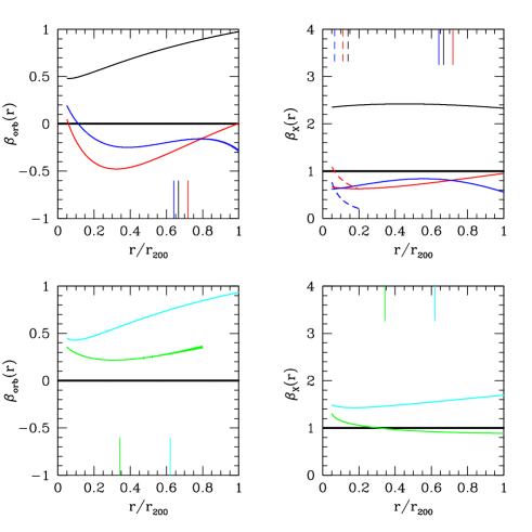
Figure 4: Velocity anisotropy parameter $\beta_{\rm orb}$ and energy ratio $\beta_{X}$. The top-left panel shows $\beta_{\rm orb}$ for the nearby clusters: A2199 (red curve), A496 (blue curve) and A576 (black curve). The top-right panel shows $\beta_{X}$ for the nearby clusters computed using ASCA/ROSAT and Chandra temperature data. Colors are as for the left panel: solid red - A2199 (ASCA/ROSAT), solid blue - A496 (ASCA/ROSAT), black - A576 (ASCA and Chandra), red dashed - A2199 (Chandra) and blue dashed - A496 (Chandra). The bottom-left panel shows $\beta_{\rm orb}$ for the high-redshift clusters. Lines are as follows: green curve - MS1358 and cyan curve - A2390. Finally, the bottom-right panel shows $\beta_{X}$ for the distant clusters (lines are as in the bottom-left panel). The vertical ticks show the maximum extent of the X-ray temperature data for the left panels. For the right panel the vertical ticks show the extent to which the mass profile is fitted. The thick line marks $\beta_{\rm orb}=0$ and $\beta_{X}=1$.

The CNOC1 group estimate the galaxy number density profiles of A2390 and MS1358 from their large spectroscopic samples including a completeness correction for galaxies without redshifts which depends on both position and magnitude (Carlberg et al. 1997). They find that the number density profiles are well fit by a Hernquist profile: [eqn.  13] with $r_{s,gxy}$=1.42 and 1.08 Mpc for A2390 and MS1358 respectively.

5 Results for the velocity anisotropy parameter

The results for $\beta_{\rm orb}$ for all five clusters are shown in the left-hand panels of Fig. 4. We find diversity in orbital parameters in our sample. Two of the clusters A2199 and A496 in the nearby sample appear to have predominantly tangential orbits in the inner region (out to 1 Mpc) as indicated by the behaviour of $\beta_{\rm orb}(r)$, whereas A576 appears to have mostly radial orbits. The distant clusters seem to be dominated by radial orbits. Computing $\beta_{X}$ using the observed temperature profile and the $\sigma_{r}^{2}(r)$ computed from the anisotropic Jeans equation, we find that MS1358 and A576 appear to deviate from hydro-static equilibrium ($\beta_{X}\neq 1$) from the inner regions to all the way out, and the rest seem to be consistent with being by-and large in hydro-static equilibrium. For A576 and MS1358, $\beta_{X}>1$ indicating less energy in the gas compared to the galaxies, whereas for A2199, A496 and A2390 $\beta_{X}\leq 1$. For A2199 and A496, the $\beta_{X}$ profiles computed from the ASCA/ROSAT temperature data are slightly higher than those from the Chandra data and have a positive slope. Henceforth, we focus on the former because of the larger spatial extent necessary for comparison with the numerical simulations. We show in Figure 5 the effect of changing the normalization of the total VDPs by $\pm$10%.

6 Comparison with cosmological simulations

We now compare the observational results for $\beta_{\rm orb}$, $\beta_{X}$ and $S(r)$ with those of high-resolution cosmological simulations based on the “concordance” flat $\Lambda\mathrm{CDM}$ model: $\Omega_{m}=1-\Omega_{\Lambda}=0.3$, $\Omega_{b}=0.021$ $h^{-2}$, $h=0.7$ and $\sigma_{8}=0.9$, where the present-epoch Hubble constant is defined as $100$ $h$ km $\mathrm{s}^{-1}$ $\mathrm{Mpc}^{-1}$, and $\sigma_{8}$ is the power spectrum normalization on $8$ $h^{-1}$ Mpc scale. The simulations are performed using the Adaptive Refinement Tree (ART) N-body+gasdynamics code (Kravtsov, Klypin & Khokhlov 1997; Kravtsov 1999; Kravtsov, Klypin & Hoffman 2002), an Eulerian code with adaptive refinement in space and time and non-adaptive refinement in mass.

To set up initial conditions we first run a low-resolution simulation of $80$ $h^{-1}$ Mpc and $120$ $h^{-1}$ Mpc boxes and select six clusters with virial masses ranging from $\approx 6\times 10^{14}$ to $1.6\times 10^{15}$ $h^{-1}{\ \rm M_{\odot}}$. The largest one has a virial mass of $1.6\times 10^{15}$ $h^{-1}$ $M_{\odot}$, the second massive cluster has a mass of $1.1\times 10^{15}$ $h^{-1}$ $M_{\odot}$, and the other four clusters have masses of $\approx 7-10\times 10^{14}$ $h^{-1}$ $M_{\odot}$. The corresponding virial radii, defined as radii enclosing the overdensity of 337 with respect to the mean density of the Universe, for the six clusters are: $2.36$, $2.10$, $2.01$, $1.93$, $1.92$, and $1.78$ $h^{-1}$ Mpc.

The initial conditions are set using multiple-mass particle technique retaining the previous large-scale waves intact but including additional small-scale waves, as described by Klypin et al. (2001). The re-sampled lagrangian region of each cluster, corresponding to a sphere of $(1.5-5)R_{\rm vir}$ around it at $z=0$, is then simulated with high dynamic range. The actual spatial resolution of the simulations is $\approx 5$ $h^{-1}$ kpc. The mass resolution (i.e., the dark matter particle mass) is $m_{p}\approx 9.1\times 10^{8}$ $h^{-1}$ $M_{\odot}$ for the all but the most massive cluster and $2.7\times 10^{8}$ $h^{-1}$ $M_{\odot}$ for the most massive cluster. The clusters thus have million or more dark matter particles within their virial radii. The simulations follow dissipationless dynamics of dark matter particles and gasdynamics of the baryonic component and include several processes crucial to galaxy formation: star formation, metal enrichment and thermal feedback due to supernovae types II and Ia, self-consistent advection of metals, metallicity-dependent radiative cooling and UV heating due to cosmological ionizing background. Stellar feedback on the surrounding gas includes injection of energy and metals via stellar winds and supernovae as well as secular mass loss (see Kravtsov, Nagai & Vikhlinin 2005, for details).

For each cluster simulation, we identify the main cluster and its galaxies using a variant of the Bound Density Maxima (BDM) algorithm using dark matter particles only. The details of the algorithm and parameters used in the halo finder can be found in Kravtsov et al. (2004). The main steps of the algorithm are identification of local density peaks (potential halo centers) and analysis of the density distribution and velocities of the surrounding particles to test whether a given peak corresponds to a gravitationally bound clump. More specifically, we construct density, circular velocity, and velocity dispersion profiles around each center and iteratively remove unbound particles using the procedure outlined in Klypin et al. (1999). We then construct final profiles using only bound particles and use these profiles to calculate properties of halos, such as the circular velocity profile $V_{\rm circ}(r)=\sqrt{GM(<r)/r}$ and compute the maximum circular velocity $V_{\rm max}$. For halos located within the virial radius of a larger host halo (the subhalos), we define the outer boundary at the truncation radius, $r_{\rm t}$, at which the logarithmic slope of the density profile constructed from the bound particles becomes larger than $-0.5$ as we do not expect the density profile of the CDM halos to be flatter than this slope. For each system we estimate the stellar mass, $M_{\ast}$, gas mass and total mass (dark matter, stars, and gas) within the truncation radius.

Once the galaxies are identified, the radial and tangential components of the velocity dispersion, $\sigma_{r}$ and $\sigma_{t}$, of the dark matter, gas and galaxies are measured in radial bins centered on the cluster potential minimum after subtracting the peculiar velocity of the cluster, defined as the mass-weighted bulk velocity of dark matter within the cluster core. Only galaxies with masses $M_{\ast}>1\times 10^{9}$ $M_{\odot}$ (or $V_{\rm max}>80$ $\rm km\,s^{-1}$) are used in this calculation. This value for the threshold provides a reasonably large sample of galaxies, while not compromising the numerical resolution of the results. The velocity anisotropy parameter $\beta_{\rm orb}$ is computed from the components of the velocity dispersion using the definition in Section 2. In addition, $\beta_{X}$ is computed using the galaxy $\sigma_{r}^{2}$ and the X-ray temperature of the gas. The measured temperatures are gas mass weighted is calculated assuming Chandra energy response in the 0.5-7 keV band. The temperature profiles in the simulations are extracted from the 3D distribution and have negligible measurement errors.

Unfortunately, the numerical results are rather noisy in the central cluster regions due to the smaller number of galaxies there. To allow a better comparison with the numerical simulations, we extend the observed $\beta_{\rm orb}$ and $\beta_{X}$ profiles to 2 Mpc by increasing the integration limit $R_{t}$ from 3.5 to 7 Mpc. Beyond 1.5 Mpc, there is a small amount of scatter in the $\beta_{\rm orb}$ profile due to numerical effects. Increasing $R_{t}$ beyond 7 Mpc slows down the calculation considerably without reducing this scatter much further, so 7 Mpc is established to be the optimal value for the large $R$ limit for the purposes of this calculation.

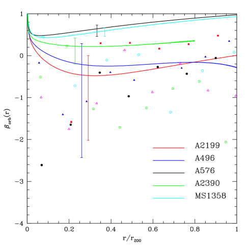
Figure 5: Velocity anisotropy $\beta_{\rm orb}$ - comparison between observations and numerical simulations. The error bars on each curve shows the error in $\beta_{\rm orb}$ due to changing $\sigma_{los}$ by $\pm 10\%$, evaluated at the given radius. The points represent the six simulated clusters.

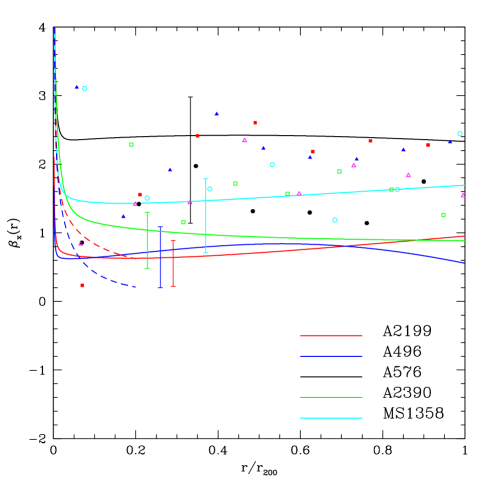
Figure 6: Energy ratio $\beta_{X}$ - comparison between observations and numerical simulations. The $\beta_{X}$’s are computed from the $\beta_{\rm orb}$ using ASCA/ROSAT temperature data for the nearby clusters and Chandra data for the distant ones. The error bars on each line show the error in $\beta_{X}$ due to changing $\sigma_{los}$ by $\pm 10\%$, evaluated at the given radius. The points represent the six simulated clusters.

The detailed results of the comparison with the simulations are discussed in the section below.

7 Discussion and Conclusions

The statistical uncertainties in the individual data points for the VDPs and the number density profiles are $\sim$20%; the uncertainties in the mass profiles are $\sim$10%. To illustrate the impact these uncertainties have on the derived galaxy orbits, we recalculate the orbital distribution $\beta_{orb}(r)$ after renormalizing the entire VDP by $\pm$10% (the uncertainty in the total VDP is smaller than the individual bins). Because the $\beta_{orb}(r)$ profiles are much more sensitive to changes in VDP than either $\nu(r)$ or $M(r)$, these uncertainties are representative of the total uncertainty from the observations (numerical errors are significantly smaller than the observational uncertainties). Figures 5 and 6 show the magnitude of these uncertainties; they are comparable to the scatter seen in the simulated clusters. The derived orbital profiles agree well with the simulated clusters, although the uncertainties in both observations and simulations are still large enough to make it difficult to distinguish mildly radial orbits from mildly circular orbits. As the observations and simulations improve, more detailed treatments of the systematic uncertainties will be required. The current study demonstrates the feasibility of this technique and the consistency of various mass estimators. That is, we successfully derive physical orbit models for the cluster galaxies assuming that they trace the mass profile inferred from independent X-ray or lensing data. We further show that these orbital profiles closely resemble those of cluster galaxies in simulations

In our cluster sample, we find a diversity of galaxy orbits. All nearby clusters appear to have primarily tangential orbits. The distant cluster MS1358 exhibits radial orbits while A2390 has predominantly tangential orbits at small radii but radial orbits at large radii ($r>1$ Mpc). The statistical uncertainties in the observed quantities can lead to large uncertainties in $\beta_{\rm orb}$: the statistical $\approx 1\sigma$ uncertainties are $\approx 20\%$ for the VDPs, $\approx 10\%$ for the mass profiles, and $\approx 20\%$ for the galaxy number densities. As an illustration, the errors plotted in Fig. 6 and Fig. 7 are calculated by changing $\sigma_{los}$ by $\pm 10\%$, while keeping the total mass and galaxy number density fixed. Because $\beta_{\rm orb}$ is much more sensitive to changes in the VDP than to the other two quantities, these errors are representative of the overall uncertainty in $\beta_{\rm orb}$ and $\beta_{X}$. Numerical errors are generally within a few per cent and much smaller than the observational uncertainties. At larger radii, where observational constraints (lensing and X-ray data) need to be extrapolated, $\beta_{\rm orb}$ is not directly constrained by the data.

We find departures from hydrostatic equilibrium in all of our clusters except A2390 (especially when the X-ray mass is used to compute $\beta_{\rm orb}$). However, these deviations are generally small ($0.6<\beta_{X}<1.6$ excluding the Chandra-based results for A2199 and A496) and comparable to the margins of error (see Fig. 6). This implies that the cluster mass estimates from X-ray observations, which are based on the assumption of hydrostatic equilibrium, may still be valid. A2199, A496 and A2390 have $\beta_{X}<1$, indicating more energy in the ICM than in the galaxies, whereas A576 and MS1358 have $\beta_{X}>1$, indicating less energy in the gas.

There is general agreement in shape, magnitude and range between the observed and simulated $\beta_{\rm orb}$ profiles (Fig. 5), especially for $r>0.5$ Mpc, where the simulations are reliable due to sufficient galaxy statistics. This agreement implies that the anisotropic Jeans equation with its assumptions of spherical symmetry is applicable to observational data. The simulated $\beta_{X}$ profiles also have similar shapes and ranges to the observed ones, but their values are approximately a factor of two larger (Fig. 6). The reason for this discrepancy is not clear. Our results are consistent with theoretical expectations that clusters are dynamically complex as they are still in the process of assembling. The difference between the inferred orbits is curious because it suggests that the moderate redshift clusters are dynamically younger than the nearby clusters. Due to the small sample size, however, it would be premature to conclude that cluster galaxy orbits evolve dramatically between $z$=0.2-0.3 and the present. If this effect is real, it could result from the observed evolution in the infall rate of galaxies (Ellingson et al. 2001).

There are several directions in which the present work could be extended. First, one could use a larger cluster sample to verify the statistical significance of the results presented in this paper - e.g. whether the differences in orbital structure between the nearby and distant clusters are a coincidence due to our small samples or a more general fact. In addition, better observational data, especially more precise cluster VDPs, would constrain the velocity anisotropy much further. The numerical simulations could also be refined in order to resolve better the central cluster regions. New sources of entropy injection could be explored with simulations that include processes such as heating by quasars and AGNs, thermal conduction and turbulent mixing.

References

- [1] Allen et al., 2001, MNRAS, 324, 877
- [2] Allen, S., Schmidt, R., & Fabian, A., 2001, MNRAS, 328, L37
- [3] Arabadjis et al., 2002, ApJ, 572, 66
- [4] Babul et al., 2002, MNRAS, 330, 329B
- [5] Bicknell et al., 1989, ApJ, 336, 639
- [6] Biviano, A. & Katgert, 2004, A&A, 424, 779
- [7] Bradac, M., Lombardi, M., & Schneider, P., 2004, A&A, 424, 13
- [8] Carlberg et al., 1997, ApJ, 478, 462
- [9] Cavaliere, A., & Fusco-Femiano, R., 1976, A+A, 49, 137
- [10] Churazov, E., Brüggen, M., Kaiser, C. R., Böhringer, H., & Forman, W., 2001, ApJ, 554, 261
- [11] Colín, P., Klypin, A.A., Kravtsov, A.V., 2000, ApJ, 539, 561
- [12] Czoske, O., Moore, B., Kneib, J.-P., & Soucail, G. 2002, A&A, 386, 31
- [13] Diaferio et al., 2005, ApJ, 628, L97
- [14] Diemand, J., Moore, B., Stadel, J., 2004, MNRAS 352, 535
- [15] Dupke, R., & White, R., 2003, ApJ, 583, L13
- [16] Fabian, A. et al., 2000, MNRAS, 318, L65
- [17] Fabricant, D.G., McClintock, J.E., & Bautz, M.W. 1991, ApJ, 381, 33
- [18] Fadda, D. et al., 1996, ApJ, 473, 670
- [19] Faltenbacher, A. et al., 2005, MNRAS, 358, 139
- [20] Finoguenov, A., Reiprich, T., & Bohringer, H. 2001, A&A, 368, 749
- [21] Fisher, D., Fabricant, D., Franx, M., & van Dokkum, P. 1998, ApJ, 498, 195
- [22] Fusco-Femiano, R., & Menci, N., 1995, ApJ, 449, 431
- [23] Gao, L., De Lucia, G., White, S. D. M.; Jenkins, A. 2004, MNRAS, 352, L1
- [24] Ghigna, S., Moore, B., Governato, F., Lake, G., Quinn, T., Stadel, J. 2000, 544, 616
- [25] Hoekstra, H., Franx, M., Kujiken, K., & Squires, G., 1998, ApJ, 504, 636
- [26] Johnstone et al., 2002, MNRAS, 336, 299
- [27] Jones, C., & Forman, W., 1984, ApJ, 276, 38J
- [28] Jones, C., & Forman, W., 1999, ApJ, 511, 65
- [29] Kempner, J., & David, L., 2004, ApJ, 607, 220
- [30] Klypin, A. and Gottlöber, S., Kravtsov, A. V., & Khokhlov, A. M., 1999, ApJ, 516, 530
- [31] Klypin, A., Kravtsov, A. V., Bullock, J. S., Primack, J. R., 2001, ApJ, 554, 903
- [32] Kneib et al., 2003, ApJ, 598, 804
- [33] Kravtsov, A. V., Klypin, A. A., & Khokhlov, A. M., 1997, ApJS, 111, 73
- [34] Kravtsov, A. V., 1999, PhD thesis, New Mexico State University
- [35] Kravtsov, A. V., Klypin, A., Hoffman, Y., 2002, ApJ, 571, 563
- [36] Kravtsov, A. V., Berlind, A. A., Wechsler, R. H., Klypin, A. A., Gottlöber, S., Allgood, B., Primack, J. R., 2004, ApJ 609, 35
- [37] Kravtsov, A. V., Nagai, D., Vikhlinin, A. A., 2005, ApJ, 625, 588
- [38] Lloyd-Davies, E.J., Ponman, T. J., & Cannon, D.B. 2000, MNRAS, 315, 689
- [39] Mahdavi, A. et al., 2005, ApJ, 622, 187
- [40] Markevitch et al., 1999, ApJ, 527, 545
- [41] Markevitch et al., 2000, ApJ, 541, 542
- [42] Mathews, W. G., & Brighenti, F., 2003, ApJ, 599, 992
- [43] McCarthy et al., 2004, ApJ, 613, 811
- [44] McNamara, B. et al., 2000, ApJ, 534, L135
- [45] Merritt, D., 1987, ApJ, 313, 121
- [46] Mohr, J. J., et al., 1996, ApJ, 470, 724
- [47] Natarajan, P., & Kneib, J.-P., 1996, MNRAS, 283, 1031
- [48] Natarajan, P. et al., 2005, MNRAS, in press, (astro-ph 0505496)
- [49] Navarro, J., Frenk, C., & White, S., 1996, ApJ, 462, 563
- [50] Nikolaev et al. 2000, AJ, 120, 3340
- [51] Piffareti, A. et al., 2005, A&A, 433, 101
- [52] Ponman, T.J., Sanderson, A.J.R. & Finoguenov, A., 2003, ApJ, 622, 187
- [53] Pratt, G.W., Arnaud, M., & Pointecouteau, E. 2005, A&A, in press (astro-ph/0508234)
- [Rines et al.(2004)Rines, Geller, Diaferio, Kurtz, & Jarrett] Rines, K., Geller, M. J., Diaferio, A., Kurtz, M. J., & Jarrett, T. H. 2004, AJ, 128, 1078
- [Rines et al.(2002)Rines, Geller, Diaferio, Mahdavi, Mohr, & Wegner] Rines, K., Geller, M. J., Diaferio, A., Mahdavi, A., Mohr, J. J., & Wegner, G. 2002, AJ, 124, 1266
- [Rines et al.(2000)Rines, Geller, Diaferio, Mohr, & Wegner] Rines, K., Geller, M. J., Diaferio, A., Mohr, J. J., & Wegner, G. A. 2000, AJ, 120, 2338
- [Rines et al.(2003)Rines, Geller, Kurtz, & Diaferio] Rines, K., Geller, M. J., Kurtz, M. J., & Diaferio, A. 2003, AJ, 126, 2152
- [Rines et al.(2001b)Rines, Mahdavi, Geller, Diaferio, Mohr, & Wegner] Rines, K., Mahdavi, A., Geller, M. J., Diaferio, A., Mohr, J. J., & Wegner, G. 2001b, ApJ, 555, 558
- [54] The, L. S., & White, S. D. M., 1986, AJ, 92, 1248
- [55] Treu et al., 2003, ApJ, 591, 53
- [56] van der Marel, R. P. et al., 2000, AJ, 119, 2038
- [57] Vikhlinin, A., Markevitch, M., & Murray, S. S., 2001, ApJ, 551, 160
- [58] Voit et al., 2003, ApJ, 593, 272
- [59] White, D., 2000, MNRAS, 312, 663
- [60] Yee, H.K.C. et al., 1996, ApJS, 102, 289
- [61] Yee, H.K.C. et al., 1998, ApJS, 116, 211
- [62] Zwicky, F., 1933, AcHPh, 6, 110
- [63] Zwicky, F., 1937, ApJ, 86, 217