A 2MASS All-Sky View of the Sagittarius Dwarf Galaxy: V. Variation of the Metallicity Distribution Function Along the Sagittarius Stream

Abstract

We present reliable measurements of the metallicity distribution function (MDF) at different points along the tidal stream of the Sagittarius (Sgr) dwarf spheroidal (dSph) galaxy, based on high resolution, echelle spectroscopy of candidate M giant members of the Sgr system. The Sgr MDF is found to evolve significantly from a median [Fe/H] $\sim-0.4$ in the core to $\sim-1.1$ dex over a Sgr leading arm length representing $\sim$2.5-3.0 Gyr of dynamical (i.e. tidal stripping) age. This is direct evidence that there can be significant chemical differences between current dSph satellites and the bulk of the stars they have contributed to the halo. Our results suggest that Sgr experienced a significant change in binding energy over the past several Gyr, which has substantially decreased its tidal boundary across a radial range over which there must have been a significant metallicity gradient in the progenitor galaxy. By accounting for MDF variation along the debris arms, we approximate the MDF Sgr would have had several Gyr ago. We also analyze the MDF of a moving group of M giants we previously discovered towards the North Galactic Cap having opposite radial velocities to the infalling Sgr leading arm stars there and propose that most of these represent Sgr trailing arm stars overlapping the Sgr leading arm in this part of the sky. If so, these trailing arm stars further demonstrate the strong MDF evolution within the Sgr stream.

1 Abundances in Dwarf Galaxies and the Halo

The idea that the stellar halo of the Milky Way (MW) formed predominantly through the infall of smaller star systems — presumably dwarf galaxies — has a long history (Searle & Zinn 1978), strong observational evidence (e.g., Majewski 1993, Majewski, Munn & Hawley 1996), and currently a strong theoretical backing by way of hierarchical, $\Lambda$CDM models (e.g., Bullock & Johnston 2005; Robertson et al. 2005; Abadi et al. 2006; Font et al. 2006). But a longstanding puzzle in this picture is why, if they are the seeds of halo formation, do MW satellite galaxies have different stellar populations (e.g., Unavane, Wyse & Gilmore 1996) and chemical abundance patterns (e.g., Fulbright 2002; Shetrone et al. 2003; Tolstoy et al. 2003; Venn et al. 2004; Geisler et al. 2005) than typical MW halo stars? One explanation (Majewski et al. 2002; Font et al. 2006) is that prolonged tidal disruption will naturally lead to evolution in the types of stars a particular satellite contributes to a halo. Indeed, it has become clear that abundance patterns (e.g., [$\alpha$/Fe]) among the most metal-poor stars in dSphs — possibly the residue of a formerly much larger metal-poor population that may have been predominantly stripped from the satellites over their lifetime — do overlap those of halo stars of the same metallicity (Shetrone et al. 2003; Geisler et al. 2005; Tolstoy 2005). But the true connection of these ancient dSph stars with Galactic halo stars remains speculative, or at least non-definitive.

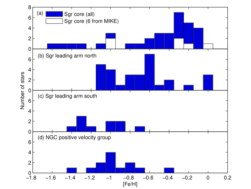
Figure 7: The MDF derived for stars in the (a) Sgr core (including all previous echelle data (Smecker-Hane & McWilliam 2002; Monaco et al. 2005) with our six newly observed stars shown in white), (b) leading arm north of the Sun, (c) leading arm south of the Sun, and (d) the positive-velocity, NGC moving group (blue circles in Fig. 1).

The Sagittarius (Sgr) dSph provides a striking example of a satellite galaxy being disrupted and slowly assimilated into the MW halo field population. It is the primary contributor of both carbon stars and M giants to the upper ($|Z_{GC}|>10$ kpc) halo (Ibata et al. 2001; Majewski et al. 2003, hereafter Paper I) and yields strong overdensity signatures of MSTO and RR Lyrae stars at halo distances (Newberg et al. 2002; Vivas, Zinn & Gallart 2005). Yet the current Metallicity Distribution Function (MDF) of the Sgr core, with median [Fe/H] $\sim-0.4$ (Fig. 7), is quite unlike that of the Galactic halo (median [Fe/H]$=-1.6$) and thus the Sgr system would seem to present one of the most dramatic examples of the apparent dSph/halo star abundance dichotomy. In this paper we explore the possible origins of this dichotomy by making high resolution, spectroscopic observations of stars not only known to have been contributed to the Milky Way halo from a specific dSph satellite, but also when. In the case of the Sgr dSph we show that the origin of the abundance dichotomy with the Galactic halo arises from preferential tidal stripping of metal poor stars, which leads to divergent MDFs between lost and retained Sgr stars, as well as a significant variation in the Sgr MDF along its tidal tails from the core to debris lost from the core several Gyr ago.

2 Previous Abundance Studies of the Sgr System

Initial photometric estimates indicated that Sgr is largely dominated by a population of old to intermediate age stars (Bellazzini et al. 1999; Layden & Sarajedini 2000), but with an MDF spanning from [Fe/H] $\sim-2.0$ to $\sim-0.5$ (see also Cacciari, Bellazzini & Colucci 2002). However, a more metal-rich population with [Fe/H] $\geq-0.5$ was found with high resolution spectra (Bonifacio et al. 2000, 2004; Smecker-Hane & McWilliam 2002; Monaco et al. 2005) as well as in a recent, deep color-magnitude diagram (CMD) from the Hubble Space Telescope ACS centered on M54 (Siegel et al. 2007). These chemical abundance studies thus present a Sgr MDF dominated by a metal-rich population with median [Fe/H] $\sim-0.4$, but having a metal-weak tail extending to [Fe/H] $\sim-2.0$ (Smecker-Hane & McWilliam 2002; Zaggia et al. 2004; Monaco et al. 2005). Monaco et al. (2003) and Cole et al. (2005) have found Sgr to have a similar MDF to the LMC (which has a dominant population of median [Fe/H]$=-0.4$) with a similar fraction of metal-poor stars, which suggests that Sgr may have had a progenitor resembling the LMC (Monaco et al. 2005). In a recent reanalysis of the age-metallicity relationship in Sgr, Bellazzini et al. (2006) find that the dSph may have enriched to near-solar metallicity as early as 6 Gyr ago, though a more recent analysis by Siegel et al. (2007) suggests a somewhat slower evolution to this enrichment level.

Thus far, abundance studies of the Sgr tails have been less detailed. Dohm-Palmer et al. (2001) obtained spectra of some K giants apparently in the northern leading arm (near its apogalacticon) and inferred the stream there was about a half dex more metal poor than the Sgr core; these authors suggested that the Sgr dSph may originally have had a strong metallicity gradient. Alard (2001) noted differences in the Sgr giant branch position in the $(J-K_{s},K_{s})_{o}$ CMD between the Sgr center and a field $7\fdg 5$ down its major axis implying a $-0.2$ dex metallicity variation between these two points (see §7). Paper I also suggested the possibility of a metallicity variation along the Sgr tidal arms because giant stars in the arms with different $(J-K_{s})_{o}$ colors seemed to yield different photometric parallax distances for the stream when the color-magnitude relation of the Sgr core was used for all colors; the differences could be explained by varying mean RGB slopes along the stream (see Figure 14 and Footnote 14 of Paper I). Adding information derived from isochrone-fitting to main sequence turnoff stars, Martínez-Delgado et al. (2004) argued that there is a substantial metallicity gradient along the Sgr stream. Vivas et al. (2005) obtained a mean [Fe/H] $=-1.77$ from low/medium resolution spectra of sixteen RR Lyrae stars in the Sgr leading arm; but since only the oldest and hence metal-poor populations in Sgr would produce RR Lyrae, this age-biased sample cannot be used to infer information on the full extent of the stream MDF. On the other hand, Bellazzini et al. (2006) found significant differences in the relative numbers of blue horizontal branch to red clump stars between the Sgr core and a position about 75^∘ forward along the Sgr leading arm, an imbalance that suggests a significant metallicity variation along the Sgr stream. Thus, while compelling evidence has been gathering for metallicity variations along the Sgr stream, no direct measurement of this variation has been made by sampling with high resolution spectroscopy the actual [Fe/H] distributions of constituent stars.

3 Observations

3.1 Sample Selection

We have begun a systematic survey of the chemical abundance patterns of stars in the Sgr stream. The goal of the present contribution is a first systematic exploration of the MDF along the Sgr stream; future work will focus on chemical abundance patterns in Sgr stream stars.

The design of our study, and in particular the rationale for the specific stars targeted for observation, has been driven by several practical considerations. First, because information on potential variations in metallicity along the stream is sought, multiple portions of the Sgr stream representing different dynamical ages (i.e. the times when the debris was stripped) is needed. Second, because the Sgr core itself exhibits a metallicity spread, insufficient information is gained by only sampling a few stars at any particular part of the tail; rather, exploration of distributions in metallicity is needed. This requires reasonable numbers of stars at each sampled section of the stream. With a limited amount of telescope time it is easier to build large samples with brighter targets, but, even focusing purely on the intrinsically brightest stars identified in the stream — the M giants explored, e.g., in Paper I and Majewski et al. (2004, “Paper II” hereafter), this is still a challenging project if spectra at echelle resolution are needed. The difficulty of securing large samples of stars partly motivated our strategy in this first study of Sgr debris stars to explore the Sgr leading arm — which passes quite near the solar neighborhood (Paper I). In contrast, the Sgr trailing arm, in its most clearly discernible parts in the southern Galactic Hemisphere, never gets closer than $\sim$15 kpc to the Sun. By observing the leading arm both just above and just below the Galactic plane we access two different points along this tidal stream with fairly local stars bright enough to take maximal advantage of our particular instrument access (two echelle spectrographs on 4-m class telescope in the Northern Hemisphere and only about one night per year on an echelle spectrograph in the Southern Hemisphere).

This strategy for exploring the leading arm, however, has some drawbacks in that (1) the trailing arm is dynamically much better understood than the leading arm (Helmi 2004; Law, Johnston & Majewski 2005, hereafter “Paper IV”), (2) the sorting of stars by dynamical age is much cleaner in the trailing arm than the leading arm (Paper IV; see also §7), (3) major sections of the leading arm are very much farther away ($\sim 50$ kpc) — out of range of our accessible instrumentation and requiring 10-m telescopes should we ever desire to “fill the gap” of our coverage of the leading arm in the same way, and (4) by focusing on rather nearby Sgr stars there is some potential for sample contamination by Milky Way disk M giants. We revisit the latter possibility in §5.

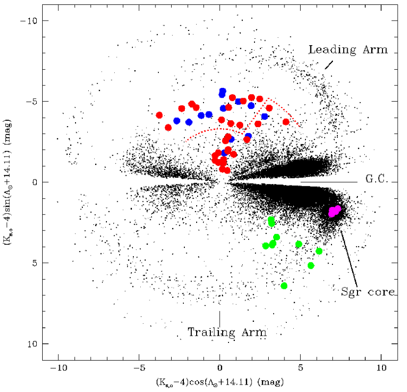
Figure 1: Sgr orbital plane position of M giants lying within 10^∘ of that nearly polar plane and having $(J-K_{s})_{o}>1.0$ and $E(B-V)<0.555$ (black dots). The Sun lies at the origin of the distribution and stars are positioned in a polar projection based on their dereddened 2MASS $K_{s}$ magnitude (radial direction, after subtraction of 4 mag) and angle from the center of Sgr, $\Lambda_{\sun}$, increasing in the direction of the trailing arm (i.e. counterclockwise). The term ($\Lambda_{\sun}+14.11$) places the intersection of the Sgr and Galactic planes horizontal across the center of the figure (see Paper I for a further description of this coordinate system). Stars from the four subsamples for which we present new data here are represented by the large colored symbols: Sgr core (magenta), leading arm north (red), leading arm south (green) and the “NGC” group of stars having positive GSR radial velocities off the main leading arm trend (blue). We do not show the positions of other stars in the Sgr core for which data are taken from the literature, but these stars lie near the magenta points in the figure. The red dotted line delineates the division of the north leading arm into the “best” (beyond the dotted line) and “less certain” (inside the dotted line) subsamples.

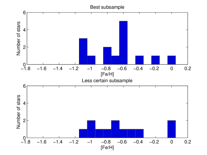
Figure 9: MDF comparison of subsamples of “leading arm north” stars, divided into the “best” (generally farther) and “less certain” (generally closer) Sgr stream groups.

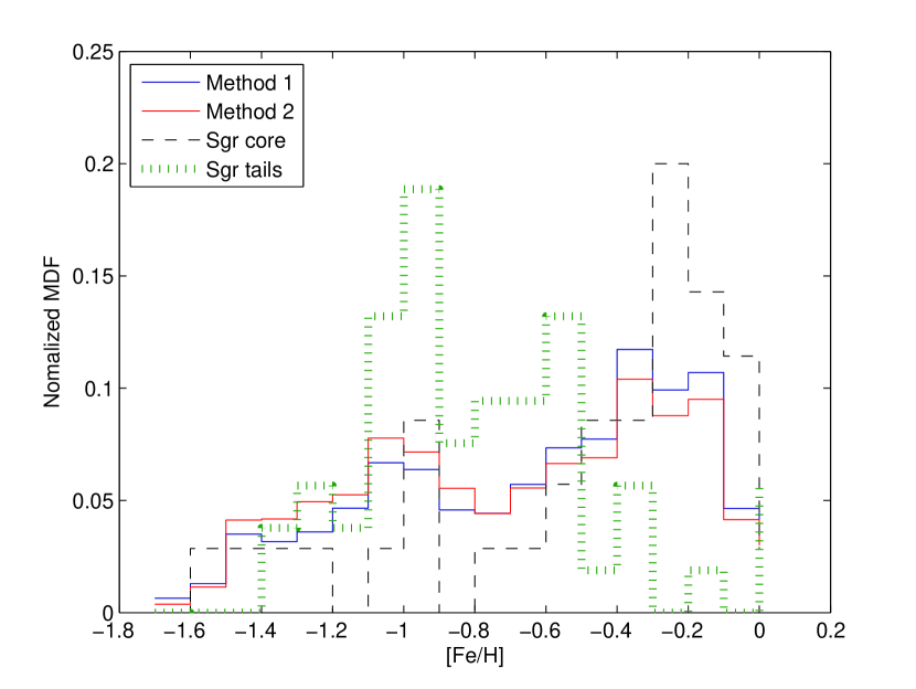
Figure 10: The approximate MDF of Sgr several Gyr ago estimated from linear combinations of those shown in Fig. 8 by the two methods described in §7 (blue lines for the first method, and red lines for the second method). The histograms have been boxcar-smoothed with a 3 bin kernal. The MDF of the Sgr core (dashed lines) and all tail stars (Figs. 8b-d, green dotted lines) are shown for comparison.

To facilitate our discrimination of Sgr stream targets from other Milky Way stars we take advantage of the ongoing studies of M giants in the stream that are the focus of this series of papers. Apart from their intrinsic luminosity, M giants confer a particular advantage in the study of the Sgr stream in that, as Paper I demonstrated, the Sgr stream has contributed the majority of the M giants found in the Milky Way halo. Thus, M giants selected far enough away from the disk already have a high likelihood of being from Sgr. Figure 1 (adapted from Fig. 9 of Paper I) shows the distribution of M giants with $(J-K_{s})_{o}>1.00$ lying within 10^∘ of the nearly polar Sgr orbital plane, as derived in Paper I. Stellar distances from the Sun (at the center) in this representation are given by the corresponding dereddened $K_{s,o}$ magnitudes. This kind of map has the benefit of creating an approximate relative spatial distribution free of biases imposed by presuming particular metallicities and color-magnitude relations needed to convert apparent magnitudes to photometric parallax distances, and works best when stars of a limited color range are used. Since most of the M giants in the figure lie in the range $1.0<(J-K_{s})_{o}<1.1$, this magnitude-based distribution reveals the basic structure of the Milky Way and Sgr stream (modulo metallicity-based variations in the absolute magnitudes of these stars), albeit with an approximately logarithmic distance scale. This log scale has the benefit not only of compressing the apparent width of the distant parts of both the Sgr leading and trailing arm, making them more visible, but of expanding the relatively small volume of space occupied by stars we have targeted in the northern Galactic hemisphere, to make their relative positions more clear. However, as pointed out in Paper I, the substantial stretching of the nearby Sgr leading arm in such a rendition makes it appear more diffuse than it really is. The reader is directed to Figures 10 and 11 in Paper I for a linear distance version of this distribution where the nearby leading arm is less “fuzzed out”, and to Figure 9 of that paper for a “clean version” (without colored dots) of the Figure 1 distribution, for comparison. The reader is also referred to Figure 1 of Paper IV for an N-body model representation of the observed debris that provides a useful guide to the expected positions of leading (and trailing) arm debris in the Sgr orbital plane.

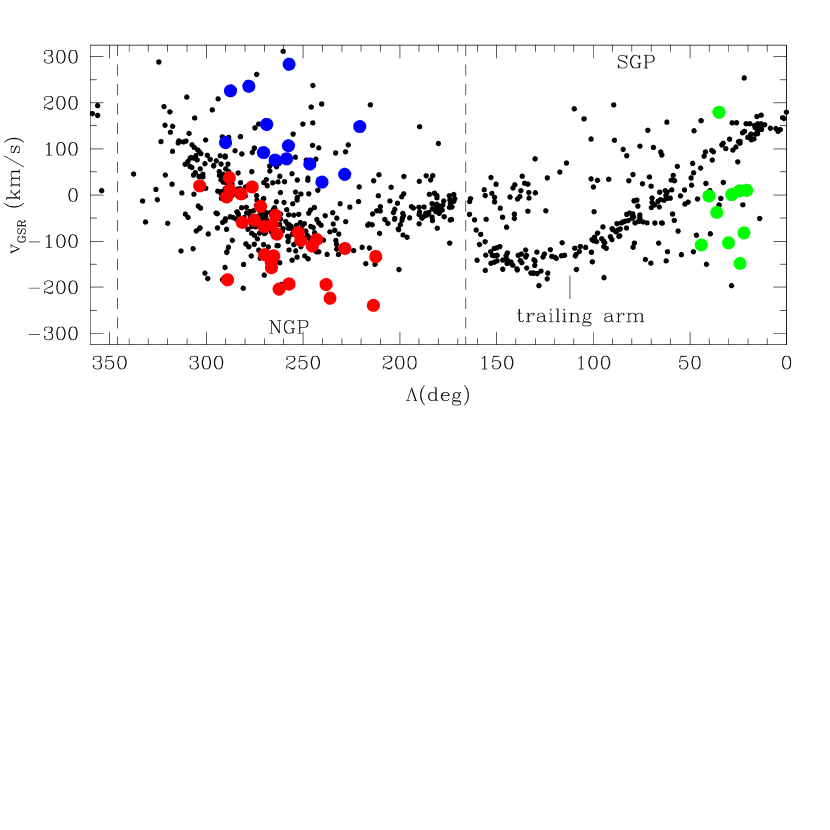
Figure 2: GSR radial velocities of stars as a function of their $\Lambda_{\sun}$ angle from Sgr center from data obtained in our ongoing medium resolution spectroscopic study. For clarity, black dots show only $(J-K_{s})_{o}>1.0$ M giants with projected distances less than 5 kpc from the Sgr orbital mid-plane and closer than 50 kpc to the Sun. The approximate $\Lambda_{\sun}$ positions of the North Galactic Pole (NGP) and South Galactic Pole (SGP) are indicated (though these actual points on the celestial sphere actually lie approximately $13^{\circ}$ off the Sgr plane being shown), as are the positions of the Galactic plane (dashed lines). The coherent velocity sequence of the Sgr trailing arm, not studied here, is also indicated. Stars from the four subsamples for which we present new data here are represented by the same colored symbols as in Fig. 1.

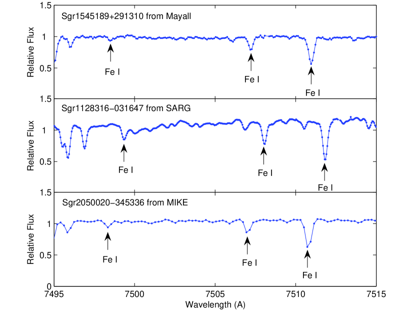
Figure 3: Sample spectra of three M giants from the three different spectrographs used in this study. Three sample iron lines are identified in the figure.

Figure 1 (and its modeled counterpart in Paper IV) provides one basis on which stars were selected for study here. But, in addition to specifically targeting M giant stars apparently positioned in particular portions of the Sgr leading arm, we also pre-select stars that have radial velocities appropriate to these positions based on Sgr debris models (Figure 10 of Paper IV) constrained to fit all available positional and radial velocity data for Sgr (e.g., Fig. 2). The velocities used for this project — both those of the stars we targeted here and those that provide the constraints for the fitted models — have been collected through an ongoing medium resolution spectroscopic survey of 2MASS M giants (Paper II, Majewski et al. in preparation; see also the data presented in Paper IV). Figure 2 shows, as a function of the Sgr orbital plane longitude ($\Lambda_{\sun}$), the observed radial velocities, converted to the Galactic Standard of Rest (GSR), of M giants lying near the Sgr orbital plane. The rather velocity-coherent trend of the Sgr trailing arm (not explored here) is obvious on the right. The RV distribution of leading arm stars is less coherent, especially where it comes close to the Sun, because of the considerable angular spread of the stream on the sky at this point (and therefore a wider variation in the projection of the stellar space motions on the line of sight). Additional RV spreading in the leading arm occurs because of the greater overlap of stars with different orbital energies at the same orbital phase compared to the trailing arm (See Fig. 1 of Paper IV). The trend of Sgr leading arm stars in Figure 2 is sinusoidal (see also Fig. 10 of Paper IV). From left to right in Figure 2: (1) Leading arm stars are first moving away from the Sgr core (at $\Lambda_{\sun}=0^{\circ}=360^{\circ}$) and have positive $v_{GSR}$ at high $\Lambda_{\sun}$; (2) after apo-Galacticon the leading arm bends towards the general direction of the Sun, and leading arm stars develop negative $v_{GSR}$ which continue to decrease as the leading arm curves towards the solar neighborhood and approaches from the general direction of the North Galactic Cap (NGC, centered near $\Lambda_{\sun}=256^{\circ}$); (3) as the leading arm traverses the Galactic plane near the Sun, the $v_{GSR}$ changes sign again with the trailing arm stars now speeding away from the solar neighborhood and arcing under the Galactic Center ($\Lambda<100^{\circ}$). It is worth noting that after passing below the Galactic plane, the leading arm crosses the trailing arm; the velocity trends of the two arms also cross in this region ($\Lambda<100^{\circ}$) as shown in Fig. 10 of Paper IV. Because the leading arm has yet another apogalacticon at $\Lambda<100^{\circ}$, the debris, and the associated velocities, is expected to become less coherent. This can be seen by the green points to the lower right of Figure 1 in Paper IV, but is not obvious by Figure 10 of that same paper, which did not show this dynamically older debris. That the overall spatial and velocity distribution of the leading arm at this point becomes more diffuse can also be seen in the models of Ibata et al. (2001; see their Fig. 3).

3.2 Spectroscopic Observations

Figures 1 and 2, and the associated figures from our models in Paper IV, guided the selection of four samples of stars for analysis here:

(1) A large sample of stars (red symbols in Figs. 1 and 2) were selected to have both positions and velocities consistent with being in the leading arm north of the Galactic plane, and in the general direction of the NGC (with Sgr longitudes $\Lambda_{\sun}$ = 220-290$\arcdeg$). Of these, 21 were observed with the $R$=$35,000$ resolution Mayall 4-m Echelle on the nights of UT 05-09 May 2004. On UT 10-13 Mar 2004, $R$=$46,000$ SARG spectra for nine additional M giants in the same part of the stream were obtained with the TNG telescope in the Canary Islands.

This “leading arm” sample is the largest in our survey, because of our mostly northern hemisphere telescope access. A large range of $K_{s,o}$ has been explored, partly because when weather conditions were non-ideal we resorted to brighter, generally closer stars. Indeed, some of the stars explored have initially projected (i.e. Paper I) distances as low as 1 kpc. Stars this close do lie among the Galactic thick disk stars, but when selecting such stars we deliberately chose stars that lie along the leading arm trend in Figure 2, and which, for the most part, have strongly negative $v_{GSR}$’s (e.g., $<-65$ km s^-1) that are unlike the typical thick disk star.

Nevertheless, as a means to explore and limit the extent to which our analysis of this leading arm sample may have been affected by thick disk contaminants that just happen to have the “right” velocity, we further divide this group even into a “best” subsample (the fainter, generally farther seventeen stars that are very highly likely to be in the Sgr leading arm) and a “less certain” subsample of thirteen stars, including those stars marked with red symbols within the boundary drawn in Figure 1. The latter subsample includes the ten leading arm north stars with $K_{s,o}<7.5$ as well as three stars at the highest $\Lambda_{\odot}$ that are closer to the Galactic bulge. If there is contamination of the leading arm north group by thick disk stars, it will most likely be among the latter sample, which has initially estimated distances from 1-5 kpc (based on the color-magnitude relation for an [Fe/H]$\sim$-0.4 population assumed in Paper I). We further discuss the issue of contamination, and the fact it is not expected to be affecting the overall conclusions of this study, in §5.

(2) Ten M giant stars with positions and velocities of leading arm stars south of the Galactic plane (green symbols) were observed with the $R$=$19,000$ MIKE spectrograph on the 6.5-m Clay telescope at Las Campanas Observatory on the night of UT 15 Aug 2005. These stars, with $\Lambda_{\sun}$ = 20-45$\arcdeg$, include stars with projected distances both inside and outside of the trailing arm and with $v_{GSR}$ well away from the trailing arm trend (Fig. 2). According to the models of Paper IV, the leading arm stars south of the Sun were predominantly stripped from Sgr roughly 2-3 Gyr ago whereas those now north of the Sun were stripped roughly 1.5-2 Gyr ago.

(3) Six stars in the very center of the Sgr core (magenta symbols) were also observed with MIKE on the same observing run as the other southern Sgr stars. Unlike the other groups of stars we looked at in this survey, these Sgr core stars were not pre-vetted based on radial velocity data, but rather selected on the basis of the infrared color-magnitude diagram. Based on the high density of Sgr giants in the core, this was a relatively safe strategy. We subsequently derived radial velocities for these stars from the MIKE spectra (values shown in Table 1), and these show them all to have radial velocities consistent with the Sgr core. These velocities were obtained via cross-correlation against four radial velocity standards using the echelle order we used for the stellar atmospheres analysis described in §4.

We combine this small sample of Sgr core stars with the other extant echelle resolution metallicities for Sgr core stars in the literature in our analysis of the MDF below.

(4) Finally, we targeted thirteen additional M giants (blue symbols) lying among the stars of the Sgr leading arm in the NGC that were found to have velocities quite unlike that expected for the Sgr leading arm at this position. We refer to this sample as the “North Galactic Cap (NGC) group”. Most of these stars are too far away and have velocities far too large to be contamination from the Galactic disk. On the other hand, while dynamically old Sgr stars from the wrapped trailing arm — if they exist in the M giant sample — are expected to lie in the direction of the NGC (Fig. 1 of Paper IV) and with more positive radial velocities, initial estimates of the distances of the NGC group stars from the Paper I photometric parallax analysis (which, again, assumes an [Fe/H]$\sim$-0.4 giant branch color-magnitude relation) puts these stars too close to the Sun to be consistent with wrapped trailing arm debris. Thus, obtaining echelle resolution spectra of some of these peculiar stars is of interest in order to test whether they can be “chemically fingerprinted” as Sgr debris (§6 and 7).

To lessen potential metallicity biases, M giant stars in all four groups were selected with a wide range of $J-K_{s}$ color — typically $\sim$1.0-1.2. Otherwise, the specific selection of targets was dictated by the desire to sample the four groups of stars outlined above and by the limitations of assigned observing schedules. Table 1 summarizes the targets, their equatorial and Galactic coordinate positions, dereddened 2MASS $K_{s}$ and $J-K_{s}$ photometry from Paper I, the Sgr orbital plane longitude ($\Lambda_{\sun}$), the velocity in the Galactic Standard of Reference ($v_{GSR}$), and the spectrograph with which each target was observed and on what date. For most stars in Table 1 we give two velocities: The first is from the medium resolution spectroscopic campaign described above (§3.1), which has typical velocity uncertainties of about 5-15 km s^-1; these are the velocities that were used in the selection of the present spectroscopic samples and that are shown in Figure 2. The second $v_{GSR}$ values were derived from the new echelle resolution spectra by cross-correlating the echelle order that we use for the chemical analyses (presented below) against that same order for several radial velocity standard stars taken from the Astronomical Almanac. The estimated velocity errors for the echelle data are 1.6 km s^-1 for the MIKE spectra, 0.6 km s^-1 for the KPNO spectra, and 0.2 km s^-1 for the SARG spectra. As may be seen, the echelle and medium resolution velocities track each other well, with a dispersion in their difference of 7.3 km s^-1, which is consistent with the uncertainties in the medium resolution spectra. In the case of the Sgr core stars we only have velocities derived from the new, echelle spectra. Table 1 also gives the $S/N$ of each spectrum; these ranged from $\sim$40-190 for the Mayall, $\sim$110-390 for the TNG and $\sim$35-120 for the MIKE data. The $S/N$ was determined using the total photoelectron count level at 7490Å.

4 Iron Abundance Analysis

4.1 Data Reduction and Equivalent Width Measurements

To convert our 2-D echelle images into fully calibrated 1-D spectra we used the basic echelle spectra reduction routines in the Image Reduction and Analysis Facility (IRAF). This process included overscan and bias correction, scattered light subtraction, flattening of the spectra by division of normalized quartz lamp exposures, extraction of the echelle orders, wavelength calibration using paired exposures of either a thorium (SARG spectra) or a thorium-argon discharge tube (KPNO and MIKE spectra) taken at the same telescope position as each target observation, and spectrum continuum fitting.

For the present analysis we focused on eleven unblended Fe I lines (listed in Table 2) found in a particular part of the spectrum previously explored by Smith & Lambert (1985; 1986; 1990 —hereafter “S&L”) in their spectroscopic exploration of M giants (see Section 4.3). We used the IRAF task splot to measure interactively the equivalent widths (EWs) of these lines, which typically spanned one echelle order.

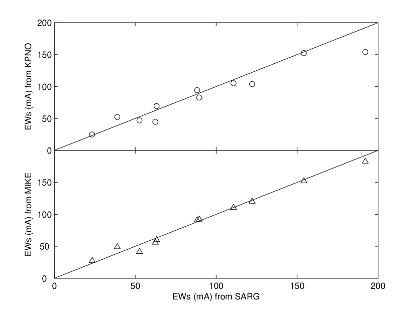
Figure 4: Comparison of Fe I line EWs among the Mayall, SARG and MIKE echelles as measured in the star Arcturus. The mean offset between Mayall and SARG is $11.00\pm 10.65$ mÅ  and $4.91\pm 3.76$ mÅ between MIKE and SARG.

Because three different instruments (with three different resolutions — see examples of spectra from each instrument in Fig. 3) were used to collect the spectra, the possibility that the equivalent widths might suffer from significant systematic differences was investigated. In Figure 4 we compare the measured EWs of Fe I lines in very high $S/N$ spectra of Arcturus (the one star we have observed on all three systems) taken on each the SARG, KPNO and MIKE spectrographs. The equivalent widths for the three different spectrographs agree reasonably well. Only slight offsets of EW(Mayall)$-$EW(SARG)=$11.0\pm 10.7$ mÅ  and EW(MIKE)$-$EW(SARG)= $4.9\pm 3.8$ mÅ  were found; because of the sizes of the uncertainties on these offsets compared to their measured values, we elected not to apply any corrections between spectrographs. However, if real, the level of these offsets in terms of an [Fe/H] value is +0.09 dex and +0.04 dex, respectively, offsets about those size of the estimated random [Fe/H] errors (see below).

The final measured EWs of the Fe I lines for each of the Sgr spectra are given in Table 3. We also include there the EW’s measured for Arcturus from spectra taken on the the three different instruments used to make Figure 4, as well as for several standard stars we analyze next.

4.2 Determining the Effective Temperatures, Surface Gravities, and Iron Abundances

A detailed abundance analysis from spectra requires as input parameters the stellar effective temperature, $T_{\rm eff}$, surface gravity (usually parameterized as $\log g$), and metallicity. The first parameter, $T_{\rm eff}$, has been determined using the dereddened 2MASS ($J-K_{\rm s}$) colors and the Houdashelt et al. (2000) color-temperature calibration. In the following analysis, the effective temperature is used in combination with stellar isochrones (Girardi et al. 2000; Demarque et al. 2004, hereafter Y²) to constrain the stellar surface gravity.

For a given population age and metallicity, a single isochrone defines a nearly unique curve in a $T_{\rm eff}$-$\log g$ plane, so that a given effective temperature defines a $\log g$ value. Red giants can either be first ascent red giant branch (RGB) stars or asymptotic giant branch (AGB) stars and these two separate phases of stellar evolution define slightly different $T_{\rm eff}$-$\log g$ tracks. However, the $\log g$ differences for a given $T_{\rm eff}$ are quite small in older stellar populations. This is particularly true for red giants with M-star temperatures ($T_{\rm eff}$$\leq$ 4000K), where the RGB and AGB almost coincide in the $T_{\rm eff}$-$\log g$ diagram (and where differences between the RGB and AGB are measured in hundredths of a dex in $\log g$).

In principle then, the effective temperature in an old red giant defines its $\log g$. The two other primary variables that define the $T_{\rm eff}$–$\log g$ curve are age and metallicity. All of the potential Sgr populations are “old”, which here translates to ages greater than about 3 Gyr. For a specific metallicity, the difference between a 3 Gyr and a 10 Gyr isochrone in a $T_{\rm eff}$-$\log g$ plane is not large (about 0.1 dex in $\log g$ at $T_{\rm eff}$=3800 K). This is due to the small difference in mass between a 3 Gyr red giant ($M\sim 1.4$ M_⊙) and a 10 Gyr one ($M\sim 1.0$ M_⊙). Once a population is older than a few Gyr, the exact age becomes relatively unimportant in defining $\log g$. Metallicity, on the other hand, does have a significant effect on the derived $\log g$ for a given effective temperature in an old red giant. This effect is incorporated into the abundance analysis here via an iterative scheme matching the isochrone used to define $\log g$ to the iron abundance then derived with that particular isochrone. Sample Fe I lines are used along with the photometric $T_{\rm eff}$ and an initial estimate of $\log g$ from an isochrone of a given metallicity to derive [Fe/H]. If this value of [Fe/H] does not match the adopted isochrone metallicity, a new isochrone is selected and the process is repeated until there is agreement between isochrone and derived spectroscopic stellar metallicity.

The Fe I lines used to determine the iron abundance and final isochrone metallicity (and thus the final $\log g$) are listed in Table 2, along with the excitation potentials and $gf$-values. The Fe I $gf$-values in Table 2 were determined by measuring these Fe I equivalent widths in the solar flux atlas of Kurucz et al. (1984) and varying the $gf$-values for each line in order to match the solar iron abundance of $A$(Fe)=7.45 (Asplund, Grevesse, & Sauval 2005). The analysis here used the LTE code MOOG (Sneden 1973) combined with a Kurucz ATLAS9 (1994) solar model, with $T_{\rm eff}$=5777 K, $\log g$= 4.438, and a microturbulent velocity, $\xi$=1.0 km s^-1.

A comparison of the Fe I $gf$-values derived in this way with those given for these same lines in Kurucz (1995) line list yields a difference of $\Delta\log gf$= +0.14$\pm$0.15. This is a small offset between these two $gf$-value scales, with a small dispersion comparable to the measured line-to-line variations found when the program stars were analyzed.

The model atmospheres adopted in the analysis were generated by interpolation from the Kurucz (1994) grids. In our iterative scheme, we also must assume an initial metallicity for the model atmosphere. Both this and the isochrone used to estimate $\log{g}$ are iterated until the derived iron abundance of the stars agrees with the metallicity of the model atmosphere, and the metallicity of the adopted isochrone.

4.3 An Analysis of Nearby “Standard” M Giants

The abundance analysis method described in the previous section can be tested on nearby, well-studied M giants that have physical properties that bracket approximately those of the program Sgr stream red giants. Included in the observed dataset for this program are three nearby M giants ($\beta$ And, $\rho$ Per, and $\beta$ Peg) that were analyzed in a series of papers by S&L. S&L focussed their studies on a narrow spectral window, near $\lambda$7440-7590Å  for abundance determinations in M, MS, and S stars. This region is quite free from significant TiO blanketing down to temperatures of about $T_{\rm eff}$=3200-3300K in giant stars, which allows for a straightforward abundance analysis. Smith & Lambert exploited this fact to explore nucleosynthesis in cool red giants on both the RGB and AGB. The same spectral region is used in this study for the Sgr stream M giants and the three bright M giants that were analyzed by S&L are analyzed here using the techniques described in Section 4.2. Along with $\beta$ And, $\rho$ Per, and $\beta$ Peg standard stars we include $\alpha$ Tau, the K5III giant used by S&L as their standard star.

As a first comparison of the spectra collected here with those from S&L, eleven Fe I lines, common to both studies, were measured in the three M giants and the mean difference in equivalent widths is found to be EW(this study)$-$EW(S&L) $=-6\pm$7 mÅ. This small offset is not significant and the scatter is about what is expected given the overall signal-to-noise levels and spectral dispersions. Spectra from this study and those from S&L are of comparable $S/N$ and resolution and have expected equivalent-width uncertainties of about $\pm$5mÅ. Differences between the two sets of measurements would then be expected to scatter around 5$\times$(2)^1/2 or $\pm$7mÅ— i.e., close to what is found.

Stellar parameters were derived for $\alpha$ Tau, $\beta$ And, $\rho$ Per, and $\beta$ Peg using first a method similar to that used by S&L, followed by the method used here for the Sgr stream stars (§4.2) to see how these different methods compare in deriving $T_{\rm eff}$, $\log g$, and [Fe/H]. S&L used ($V-K$) colors to define $T_{\rm eff}$, while they set the luminosity based on the Wilson (1976) calibration of the strength of the Ca II K-line with absolute visual magnitude ($M_{\rm V}$). Given luminosity and effective temperature, S&L then compared these observed values to stellar-model mass tracks to set $\log g$ via the relation of $g\propto(M\times L)/T_{\rm eff}$⁴.

One significant difference between this particular S&L procedure and our modified use of it here concerns the estimate of the luminosities. The S&L studies predate the availability of Hipparcos parallaxes, which are now well-measured for the four red giants under consideration. Table 4 lists the Hipparcos parallaxes for $\alpha$ Tau, $\beta$ And, $\rho$ Per, and $\beta$ Peg, as well as the resulting distances (and their respective uncertainties). These distances then provide the absolute $V$- and $K$-magnitudes also listed in the table (with the distance uncertainties considered). Both $V$ and $K$ bolometric corrections were applied to determine $M_{\rm bol}$ in Table 4, with the respective corrections differing by less than 0.05 in magnitude. Finally, effective temperatures from both a ($V-K$) calibration (Bessell et al. 1998) and the ($J-K$) calibration from Houdashelt et al. (2000) are listed in Table 4.

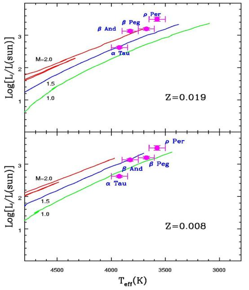
Figure 5: Stellar luminosities versus effective temperatures for the four standard red giants are calculated by assuming $M_{\rm bol}$=4.74 for the Sun. Also plotted in this figure are stellar model tracks from the Padua grid for masses of $M$=1.0, 1.5, and 2.0M_⊙. The top panel shows models with near-solar metallicity ($Z$=0.019), while the bottom panel has models with [M/H]$\sim$-0.4 ($Z$=0.008).

Stellar luminosities for the four standard red giants are calculated by adopting $M_{\rm bol}$=4.74 for the Sun and the values of $\log$($L$/L_⊙) versus the mean $T_{\rm eff}$ (i.e. the average of the two determinations in the previous paragraph) are plotted in the two panels of Figure 5. Also plotted in this figure are stellar model tracks from the Padua grid for masses of $M=$1.0, 1.5, and 2.0M_⊙. The top panel shows models with near-solar metallicity ($Z=$0.019), while the bottom panel has models with [M/H]$\sim=-0.4$ ($Z$=0.008). This figure illustrates the effect that metallicity has on estimates of the gravity. At lower metallicities the model tracks indicate a lower mass for a given measured $T_{\rm eff}$ and $\log L$. This effect is quantified in Table 5 where $T_{\rm eff}$ and $\log L$/L_⊙ are listed, along with the estimated mass and resultant $\log g$ for the two model metallicities plotted in Figure 5.

Given the effective temperatures and model mass (and thus $\log g$) as a function of metallicity, the Fe I equivalent-widths are used in an abundance analysis to achieve final agreement between derived [Fe/H] and model metallicity. In the line analysis the microturbulent velocity is set by the requirement that the derived Fe abundance be independent of the Fe I equivalent width for the different lines. The derived values of $\log g$, microturbulence ($\xi$) and [Fe/H] are listed in Table 5. These values of $\log g$ can be referred to as “Hipparcos gravities” because they are set by the mass, which is derived from the luminosity, which is derived from the distance, which is derived from the Hipparcos parallaxes. This analysis is very similar as that used by S&L, differing only in that S&L used Ca II K-line absolute magnitudes to establish a luminosity while here the Hipparcos parallaxes are used to get a distance and therefore a luminosity.

With the basic red giant parameters now defined for the bright giant stars via the standard Fe-abundance analysis, the new analysis technique (§4.2) used in this paper for the candidate Sgr stream red giants can be checked for differences when also applied to these same bright giant stars. Recall that with Sgr stream stars there is no reliable distance estimate available to establish luminosity; rather, the effective temperature is used in combination with the Fe abundance to establish surface gravity via isochrone tracks. Moreover, for the new analysis the $T_{\rm eff}$ are derived only from ($J-K$) colors (rather than from both $J-K$ and $V-K$ colors) due to the larger effects of uncertain reddening on optical colors and also the fact that we don’t have $V-K$ colors for the Sgr stream giants. Finally, we apply several different isochrone ages as well as two separate families of isochrones (Girardi et al. 2000 versus $Y^{2}$) in the characterization of the standard red giants to test the sensitivity of the new technique to these variables. The results of the “new” analysis applied to the bright giants are tabulated in Table 6.

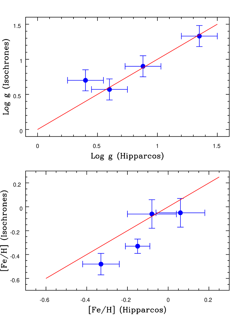
Figure 6: A graphical comparison of surface gravities (top panel) and [Fe/H] values (bottom panel) derived from the Hipparcos parallaxes and the isochrone method for the four bright standard stars analyzed in §4.3.

The Table 6 results show, first, that there is rather little difference in the derived surface gravities to either the adopted set of isochrones or the variation from 1.0 Gyr to 2.5 Gyr isochrones. We have already mentioned (§4.2) that there is only a $\log g$ difference of 0.1 between a 3 and a 10 Gyr isochrone of the same metalliticity; the 1 and 2.5 yr isochrones here are intended to explore ages more appropriate to disk-like giants like our standard stars, but we note that there is only a $\Delta\log{g}$ difference of 0.05 between a 2.5 and a 5 Gyr isochrone of the same metallicity. Moreover, a comparison between the Table 6 gravities and abundances and those derived from the more standard analysis reveals no large differences. Figure 6 provides a graphical comparison of the surface gravities (top panel) and [Fe/H] (bottom panel) derived from the two techniques, and shows their close correlation.

This comparative analysis of the four red giants with well-established, fundamental stellar parameters demonstrates that the analysis technique used for the candidate Sgr Stream red giants is sound, and yields reliable stellar parameters and Fe abundances.

4.4 Final Results

Table 7 gives the results of the §4.2 abundance analysis applied to our Sgr stars. For each star, the columns give the derived effective temperature using the Houdashelt et al. (2000) color-temperature relation applied to the 2MASS $(J-K_{s})_{o}$ color, and the derived values of the surface gravity ($\log{g}$), microturbulence and [Fe/H]. In the case of the surface gravities, any entry given as “0.0(-)” means that our iterative procedure was converging on a model atmosphere with $\log{g}<0$, whereas the Kurucz (1994) model atmosphere grids do not go below $\log{g}=0$. In these cases, we have adopted the $\log{g}=0$ atmosphere.

The final column in Table 7 represents the standard deviation in the line abundance determinations. In principle, from the adopted model atmosphere and each EW we get a measure of the abundance. With multiple EWs from different Fe I lines, MOOG calculates the standard deviation of the resulting abundances. The typical standard deviations are about 0.1 dex. Combined with the instrument-to-instrument offsets discussed in §4.1 and shown in Figure 4 as well as other potential offsets, such as those shown in Figure 6, we estimate the full [Fe/H] errors, systematic and random combined, to be no more than $\sim 0.2$ dex.

5 Metallicity Distribution Functions

5.1 The Sagittarius Core

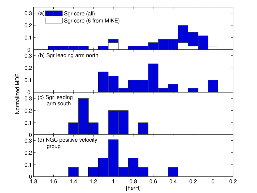
Figure 8: Same as Figure 7, but with each panel scaled to the same “normalized MDF” scale.

Figures 7 and 8 summarize the MDFs determined for the three groups of Sgr core/leading arm samples studied here (Figure 7 shows the distributions with the same absolute vertical scale, Figure 8 shows the distributions with the same normalized, fractional MDF scale in each panel).

For the Sgr core, data for our six stars (Figs. 7a and 8a; shown by the open histogram) have been combined with previous echelle data for 14 K giants by Smecker-Hane & McWilliam (2002) and for 15 M giants by Monaco et al. (2005). The precisions in the metallicities quoted for each of these studies is 0.07 and 0.20 dex, respectively, similar to our results here. The combined MDF from these data shows the very broad distribution previously reported for Sgr (see §2), with a peak near [Fe/H]=-0.3 but a very long, metal-weak tail. The new MIKE spectra we collected contribute two stars near [Fe/H] = -1 but the other four lie in the metal-rich end of the distribution, and include one star we determine to have solar [Fe/H]. We consider this star to be a bona fide member of Sgr because of its chemical peculiarities (in particular, its Ti, Y, and La abundances, which are like other Sgr stars of similar metallicity, as we shall show elsewhere — Chou et al., in preparation).

5.2 Leading Arm North

Panels (b) in Figures 7 and 8 present the MDF for all stars we selected to be members of the Sgr leading arm in the Northern Hemisphere. As may be seen, while broad like the MDF of the Sgr core, the distribution “of leading arm north” stars is, on the whole, more metal poor than the Sgr core, with a median near -0.7 dex.

As discussed in §3, this particular sample is the most vulnerable to potential contamination by Milky Way disk M giants. However, several arguments can be made that this contamination is probably small, and, even if there is some contamination, it has little affect on the overall conclusions of the present study:

(1) First, we can compare the MDFs of subsamples of “leading arm north” stars, divided into the “best” (generally farther) and “less certain” (generally closer) Sgr stream groups discussed in §3. Figure 9 makes this comparison, and shows that there is little difference in the overall character of the two MDFs. The two subsamples have the same median [Fe/H] and similar tails to the metal-rich end. The difference in the mean metallicities of the two samples, -0.72 and -0.64 dex, respectively, is much smaller than the MDF dispersions (0.31 and 0.33 dex, respectively).

(2) The majority of the stars in the Leading Arm North sample are more metal-poor than the mean metallicity of the Sgr core, so that their projected distances are even farther away from the Milky Way disk than initially projected based on the Paper I photometric parallaxes that assumed a Sgr core RGB color-magnitude relation. For the “best” subsample, the implied minimum distances are generally 10 kpc or more, well above the Galactic disk.

(3) The median metallicity of the Galactic thick disk, the Milky Way component most likely to contribute contaminants, is well known to be about -0.7 dex (whereas the thin disk would contribute more metal rich stars in general, if at all). Thus, we might expect the probability distribution of Milky Way contaminants to look very similar to the distribution we actually see, and therefore have little impact on the true MDF.

(4) As we shall show elsewhere (Chou et al., in preparation), the abundance patterns (e.g., the combinations of [Fe/H], [Ti/Fe], [Y/Fe], [La/Y]) of all but a few of the stars in the leading arm north sample (and indeed in our entire survey) are quite unlike those of Milky Way stars, but very much resemble the patterns seen in dSph stars, including Sgr (Bonifacio et al. 2000; Fulbright 2002; Smecker-Hane & McWilliam 2002; Shetrone et al. 2003; Venn et al. 2004; Geisler et al. 2005; Monaco et al. 2005).

(5) The leading arm stars were pre-selected to be in the Sgr stream and to follow the expected velocity trends for Sgr debris. No evidence for other M giant tidal debris from any other satellite is found to intersect the Sgr stream. Because the bulk of the halo M giants are found to be contributed from the Sgr system and we are probing the general orbital plane of the Sgr system and well away from the Galactic disk for the most part, it is logical to conclude that our leading arm samples (both north and south) are indeed dominated by members from the Sgr dSph.

Thus, we expect the relative contamination of our leading arm north sample by Milky Way stars to be small. While at this point it is true that we cannot be assured that every star in any of samples, or any one particular star within them, is definitely a member of the Sgr stream, a few contaminants will have little effect on the general conclusions of this paper, which are based on mean trends in the Sgr MDF. In this regard, it is sufficient that most of the stars are Sgr stream members and to recognize that the Leading Arm North MDF differs significantly from that of the Sgr core.

5.3 Leading Arm South

The Leading Arm South sample (Figures 7c and 8c) shows an even more metal-poor MDF than either the Sgr core of the Leading Arm North samples. With regard to contamination by the Milky Way disk, things are even more secure for this sample than for the Leading Arm North: Not only are these stars even farther away from the disk according to the original projected distances from Paper I (and even more so if their projected distances are corrected for their newly discovered low metallicity), but they have an MDF even more unlike the Milky Way disk. The median metallicity of around -1.1 dex, the lack of stars more metal rich than [Fe/H]=-0.7, the relatively small [Fe/H] dispersion in this sample, and unusual chemical abundance patterns found in these stars (Chou et al., in preparation) all argue against the notion of significant contamination of this group of stars by the thick disk.

5.4 Evolution in the Sagittarius MDF

Comparison of the Sgr core MDF with those at the two points in its leading arm we explored here (Figs. 7b/8b and 7c/8c) reveals substantial evolution in the Sgr MDF with position. While all three points of the Sgr system sampled contain stars from a metal-poor population with [Fe/H] $<-1$, the relative proportion of these stars increases with separation from the Sgr core. The latter shows a dominant metal-rich population peaked at [Fe/H] $\sim-0.3$, whereas the median metallicity declines from $\sim-0.4$ dex in the core to $\sim-0.7$ dex in the leading arm north of the Sun and $\sim-1.1$ dex south of the Sun, which represents debris lost from the Sgr core some 3.5 orbits ($\sim 2.5-3$ Gyr) ago (Paper IV).

While the Figure 7c/8c MDF has only one star with [Fe/H]$>-0.95$, because we are color-selecting M giants our samples tend to be biased against finding metal-poor giants (which are bluer and earlier in spectral type). Thus the significant, $-0.7$ dex median metallicity gradient shown in Figures 7 and 8 may actually underestimate the true gradient of what already appears to be a substantial MDF variation along the Sgr stream. We address the implications of this gradient in §7.

6 Evidence for Sgr Trailing Arm in the North

In the course of our ongoing, medium resolution radial velocity survey of Sgr M giants (e.g., Majewski et al. 2004) we identified a subsample of M giants lying among leading arm stars at the NGC, but having the opposite velocity expected for falling leading arm debris there (see $v_{\rm gsr}>0$ black points near $\Lambda_{\sun}$ = 260$\arcdeg$ in Fig. 12 of Paper IV). Because of their apparent proximity to the Sun (solid blue points, Figs. 1 and 2), the origin of these stars has been puzzling. Thirteen of these peculiar velocity M giants with median $\Lambda_{\sun}$=265$\arcdeg$ were targeted with the Mayall 4-m and TNG SARG echelle spectrographs on the same observing runs and to the same approximate $S/N$ as the NGC leading arm stars (§3).

The relatively low metallicities of these $v_{\rm gsr}>0$ stars (Figs. 7d/8d) indicates that the initial Paper I photometric distances for these stars (based on an assumed [Fe/H]$\sim-0.4$; Fig. 1) were underestimated by a mean factor of $\sim 1.5$, based on the color-magnitude sequences presented in Ivanov & Borissova (2002). Adjusting the distances for correct metallicities — minding the $v_{\rm gsr}$ of these stars and recognizing that the models were not well constrained for old debris — we find reasonable consistency of these stars with the Sgr trailing arm towards the NGC (see Fig. 12 of Paper IV).

Detailed abundance analysis supports this conclusion. The MDF of these positive $v_{\rm gsr}$ stars (Figs. 7d/8d) fits the general trend with Sgr mass loss epoch established by the leading arm data (Figs. 7a-c/8a-c); as may be seen by comparing the mass loss epoch sequences of the leading and trailing arms in the Paper IV (colored point in Figure 1) model, stars in our leading arm south sample and in the NGC sample, if it is indeed old trailing arm debris, were torn from Sgr at approximately the same time. Thus it is compelling that the MDFs in Figures 7c/8c and 7d/8d look very similar to one another. In addition, this NGC moving group is found to have similarly peculiar Ti , Y  and La  abundance trends as stars in the Sgr leading arm (Chou et al., in preparation), further supporting the idea of a common origin with these latter stars.

If trailing arm stars are found toward the NGC it establishes with certainty that the Sgr debris tracks at least 3 orbits (2.5-2.75 Gyr) of mass loss (Paper IV); because of much stronger phase mixing of debris in the leading arm, this fact is not well established by the apparent length of the Sgr leading arm (although previous evidence that it may exist has been offered by Martinez-Delgado et al. 2004). Moreover, including the MDF in Figures 7d/8d in the overall sequence shown in Figures 7a-c/8a-c, lends further support to the overall notion that there is a significant MDF variation along the Sgr stream.

7 Discussion

Because Sgr is reputed to have enriched to near solar metallicity by at least a few Gyr ago (Lanfranchi & Matteucci 2004; Bellazzini et al. 2006; Siegel et al. 2007), the observed MDF variation over the past 3.5 orbits (2.5-3 Gyr) of mass loss cannot be due to an intrinsic variation of the instantaneous mean metallicity of the Sgr system with time. Rather, it must point to the shedding of successive layers within the satellite over which there must have been an intrinsic MDF gradient (see also Martínez-Delgado et al. 2004). However, the $>0.7$ dex median metallicity variation in the debris lost over a 2.5-3 Gyr timescale is quite large and suggests the loss of stars over a significant radius in the system. For comparison, the strongest [Fe/H] gradient observed in the Sculptor dSph is about 0.5 dex over about $0\fdg 2$ ($\sim 275$ pc), which is about 15% the apparent Sculptor tidal radius; however, this same 0.5 dex change also represents the entire variation seen across the $\sim 75\%$ of the Sculptor tidal radius studied in detail so far (Tolstoy et al. 2004). Sculptor seems to have among the strongest net internal metallicity gradients among Milky Way dSphs (though some M31 dSphs may have larger gradients; Harbeck et al. 2001); for comparison, the now well-studied Carina dSph exhibits only a $-0.2$ dex gradient from its core to its tidal radius (Koch et al. 2006). Moreover, no large metallicity gradient seems to exist within the main body of Sgr now: Alard (2001) identified only a $-0.2$ dex variation in mean metallicity from the Sgr core to $7\fdg 5$ down the major axis. While the position of the current tidal radius in Sgr is still uncertain, Paper I argues that it is likely to be only $\sim$ 3-4$\arcdeg$ (or Sgr would be too massive to produce its observed dynamically cold tails); thus the Alard observation likely pertains to the beginning of the metallicity gradient within the debris tail. Therefore, we must conclude either (1) the destruction of Sgr over the past several Gyr has been fine-tuned to mass shedding from a narrow progenitor radial range over which there was an extraordinarily strong [Fe/H] gradient for a dSph, or, (2) more likely, Sgr experienced a quite rapid change in its binding energy over the past several Gyr, which has decreased the tidal boundary of the satellite across a broader radial range over which there would have still been a large net metallicity variation, but a shallower and more typical gradient. Such a catastrophic change of state happening so relatively recently (1/5 the Hubble time) points to a dramatic event affecting Sgr’s life several Gyr ago, perhaps a transition to its current, destructive orbit.

Figures 7 and 8 not only provide the first direct evidence that the satellites of today may not well represent the stars they lost to the halo, but that this effect can be considerable. If tidal mass loss is typical among other dSph systems, as seems to be the case (e.g., Muñoz et al. 2006a, 2007; Sohn et al. 2007), it might explain such puzzles as why: (1) the detailed chemical abundances (e.g., [$\alpha$/Fe] vs. [Fe/H]) of satellites today appear to differ from those observed in the halo field to which they should contribute (e.g., Font et al. 2006), (2) a system like the Carina dSph, which exhibits clear signs of tidal disruption, presently holds a much larger fraction of intermediate-age than old stars today (Majewski et al. 2000, 2002), and (3) there remains a G dwarf problem in dSph systems (e.g., Koch et al. 2006; Helmi et al. 2006). Such mass loss shaping of the MDF prompts caution in attempting to interpret the chemical evolution and star formation history of a dSph based on stars left in its core (e.g., Tolstoy et al. 2003; Lanfranchi & Matteucci 2004).

To demonstrate this point, we approximate the total MDF of the Sgr core several Gyr ($\sim$3.5 orbits) ago using two methods to account for stars now in the tidal streams produced over that time. In the first method (Fig. 10, blue lines), the normalized MDFs in Figs. 8a-c represent their respective median Galactocentric orbital longitudes and each leading arm star (as identified in Fig. 11 of Paper I) is assigned a longitude-interpolated version of these different MDFs. Regions obscured by the Galactic plane or overlapping trailing arm are “filled in” by reflecting the numbers of stars in the corresponding part of the trailing arm as seen from the Galactic Center (in the case of the first $50\arcdeg$ of leading arm) or by extrapolating the observed stream density (for the farthest 175-300$\arcdeg$ of leading arm – i.e. that part starting in the solar neighborhood). In the second method (Fig. 10, red lines) we use the Sgr disruption model for an oblate Milky Way halo from Fig. 1 of Paper IV and assign the normalized MDFs in Figs. 8a, b and c to leading arm model stars lost on the last 0.5 orbit (i.e., since last apogalacticon; yellow-colored debris in Fig. 1 of Paper IV), 1.5-2.5 orbits ago (cyan-colored debris) and 2.5-3.5 orbits ago (green-colored debris) respectively, while for debris lost 0.5-1.5 orbits ago (magenta-colored debris) we use the average of Figures 8a and b. The model provides the relative numbers of stars in each Sgr population (bound and unbound). Both “Sgr-progenitor” MDFs generated are relatively flat, exhibiting a much higher representation of metal-poor stars than presently in the Sgr core. These regenerated MDFs are, of course, necessarily schematic, because (1) The [Fe/H] spread of the net MDFs is, of course, limited by the input MDFs, (2) an M giant-based survey is biased against finding metal-poor stars, and (3) Sgr stars with [Fe/H]$\sim-2$ have already been reported (see §1; ironically, the most metal poor stars shown in Fig. 7 are contributed by the input MDF of the Sgr core, which includes bluer giants as well as a larger overall sample of stars that allows a higher chance of drawing stars from a low probability, metal-poor wing in the distribution). But Figure 10 illustrates how critically the observed MDFs of satellite galaxies may depend on their mass loss/tidal stripping history.

We have discussed integrated MDFs as a function of position in the Sgr system, but it is likely that, like other dwarf galaxies, Sgr has had a variable star formation history including possible “bursts” (Layden & Sarajedini 2000; Siegel et al. 2007), and that these produced populations with different, but overlapping radial density profiles in the progenitor satellite. The MDF gradients described here may relate more to differences in the relative proportion of distinct populations than a smooth variation in mean metallicity from a more continuous star formation history. “Distinct” Sgr populations are suggested by the multiple peaks and general character of the Figure 7 MDFs (and even more strongly by stream position variations of the abundances of other elements, like lanthanum; Chou et al., in prep.). Earlier suggestions of multiple Sgr populations include Alard (2001), Dohm-Palmer et al. (2001), Smecker-Hane & McWilliam (2002), Bonifacio et al. (2004), and Monaco et al. (2005). Greater resolution of the initial Sgr stellar populations, their former radial distributions, and the Sgr enrichment history will come from further scrutiny of its tidal debris, particularly along the trailing arm. As shown in Figure 1 of Paper IV, leading arm stars lost on different orbits (i.e., shed from different radial “layers”) significantly overlap in orbital phase position; this “fuzzes out” the time (i.e. initial satellite radius) resolution. In contrast, the dynamics of the longer trailing arm yields much better energy sorting of the debris, and stars stripped at specific epochs can be more cleanly isolated. In addition, study of the trailing arm will allow much better separation of the Sgr debris from potential Milky Way disk M giant contamination.

The abundance gradients found here imply that the estimated photometric distances for many M giant stars along the Sgr tidal arms have been systematically underestimated in Paper I, where photometric parallaxes were derived using the color-magnitude relation of the Sgr core. The best-fitting Sgr destruction models of Paper IV should now be refined to account for this variation (as well as an updated distance for the Sgr core itself — e.g., Siegel et al. 2007). Proper spectroscopic parallax distances will necessarily require assessment of both [Fe/H] and [$\alpha$/Fe] to determine absolute magnitudes. We undertake this task elsewhere.

Table 1: The Program Stars

Star ID	$\alpha$(2000)	$\delta$(2000)	$l$	$b$	$K_{s,o}$	$(J-K_{s})_{o}$	$\Lambda_{\odot}$	$v_{\rm gsr}$(old/new)	Spectrograph	Observation	$S/N$
	(deg)	(deg)	(deg)	(deg)			(deg)	(km s-1)		UT Date
Sgr Core
$1849222-293217$	82.34253	-29.53815	5.98090	-12.58070	11.481	1.00	358.63837	135.9	MIKE	2005 Aug 15	34
$1853333-320146$	283.38861	-32.02935	4.00803	-14.40648	11.240	1.05	359.97171	164.5	MIKE	2005 Aug 15	51
$1854283-295740$	283.61789	-29.96109	6.04514	-13.76432	11.180	1.06	359.80359	162.3	MIKE	2005 Aug 15	43
$1855341-302055$	283.89218	-30.34867	5.77648	-14.13644	11.392	1.03	0.10415	152.6	MIKE	2005 Aug 15	74
$1855556-293316$	283.98166	-29.55454	6.55899	-13.89102	11.230	1.09	0.04467	173.9	MIKE	2005 Aug 15	45
$1902135-313030$	285.55618	-31.50829	5.24634	-15.90276	11.198	1.06	1.70370	158.8	MIKE	2005 Aug 15	55
Sgr North Leading Arm — Best Subsample
$0919216+202305$	139.83992	20.38467	208.89221	41.35083	8.663	1.09	212.41455	-133.5/-125.4	ECHLR	2004 May 07	74
$0925364+213807$	141.40163	21.63516	207.89902	43.12523	9.592	1.17	213.68213	-239.4/-215.4	ECHLR	2004 May 07	54
$1034395+245206$	158.66466	24.86820	209.33199	59.27583	9.140	1.11	228.44516	-116.0/-102.3	ECHLR	2004 May 09	62
$1100516+130216$	165.21519	13.03777	236.02568	60.56746	8.856	1.04	238.10635	-194.1/-186.5	ECHLR	2004 May 06	77
$1101112+191311$	165.29662	19.21981	224.41052	63.52243	9.146	1.07	236.06346	-223.8/-219.2	ECHLR	2004 May 06	73
$1114573-215126$	168.73872	-21.85714	275.07312	35.74147	7.864	1.22	257.30670	-193.0/-198.0	ECHLR	2004 May 06	72
$1116118-333057$	169.04900	-33.51587	281.07785	25.28218	7.697	1.15	266.35822	-157.7/-140.6	ECHLR	2004 May 09	46
$1140226-192500$	175.09427	-19.41671	280.73941	40.37285	8.663	1.03	262.44983	-204.1/-205.2	ECHLR	2004 May 06	80
$1249078+084455$	192.28256	8.74870	301.12396	71.61227	9.295	1.05	264.23920	-44.1/-53.6	ECHLR	2004 May 05	56
$1318500+061112$	199.70825	6.18672	321.43869	68.06859	9.229	1.02	271.92865	-24.7/-31.3	ECHLR	2004 May 06	70
$1319368-000817$	199.90341	-0.13814	318.02545	61.90507	7.741	1.22	275.23373	-54.7/-41.6	ECHLR	2004 May 05	63
$1330472-211847$	202.69652	-21.31316	315.03806	40.63177	8.310	1.01	289.06110	-183.8/-181.5	ECHLR	2004 May 09	41
$1334532+042053$	203.72151	4.34796	329.30008	64.97141	9.598	1.08	276.31186	17.4/23.3	ECHLR	2004 May 06	57
$1411221-061013$	212.84189	-6.17026	336.00510	51.49488	9.512	1.08	289.51416	-4.4/-6.7	ECHLR	2004 May 09	61
$1450544+244357$	222.72687	24.73260	34.60439	63.09545	9.713	1.03	281.42078	-59.5/-66.6	ECHLR	2004 May 06	61
$1456137+151112$	224.05695	15.18672	16.93899	58.66600	7.122	1.05	288.11844	37.4/33.3	SARG	2004 Mar 11	128
$1512142-075250$	228.05925	-7.88056	352.23251	41.13720	9.531	1.11	303.44876	19.7/4.3	ECHLR	2004 May 05	65
Sgr North Leading Arm — Less Certain Subsample
$1111493+063915$	167.95526	6.65415	249.26958	58.71890	5.387	1.15	243.01091	-96.4/-93.6	SARG	2004 Mar 11	367
$1112480+013211$	168.19978	1.53646	256.03873	55.16073	5.673	1.04	245.24609	-110.8/-135.4	ECHLR	2004 May 07	124
$1128316-031647$	172.13158	-3.27976	266.38379	53.60342	5.230	1.09	251.16019	-98.1/-98.6	SARG	2004 Mar 11	376
$1135388-022602$	173.91154	-2.43394	268.24146	55.24917	5.825	1.10	252.52528	-81.3/-78.4	SARG	2004 Mar 11	267
$1208101-090753$	182.04225	-9.13136	285.31238	52.25384	6.595	1.07	263.57907	-84.8/-85.9	SARG	2004 Mar 11	169
$1223590-073028$	185.99593	-7.50770	291.09094	54.73156	4.820	1.16	266.45792	-146.1/-144.3	ECHLR	2004 May 06	174
$1224255-061852$	186.10632	-6.31443	290.89117	55.92445	6.864	1.05	265.95511	-64.8/-64.7	SARG	2004 Mar 13	216
$1227367-031834$	186.90295	-3.30937	291.31927	59.02406	5.422	1.01	265.19498	-132.0/-131.8	ECHLR	2004 May 06	163
$1236549-002941$	189.22878	-0.49475	295.13962	62.15701	5.198	1.06	265.93793	-137.9/-137.0	ECHLR	2004 May 06	190
$1348366+220101$	207.15269	22.01685	14.56112	76.04436	5.981	1.02	270.13049	-68.5/-75.0	SARG	2004 Mar 11	284
$1407060+063311$	211.77515	6.55299	347.49780	62.68076	5.924	1.12	282.12589	2.5/-5.1	SARG	2004 Mar 13	160
$1435018+070827$	218.75742	7.14080	358.56470	58.32960	4.856	1.11	287.82812	10.8/3.5	SARG	2004 Mar 11	390
$1538472+494218$	234.69650	49.70488	79.71546	50.95237	6.076	1.16	269.88177	-129.4/-132.1	ECHLR	2004 May 05	65
Sgr South Leading Arm
$2031334-324453$	307.88907	-32.74802	10.20659	-34.28811	11.480	1.04	20.63735	10.3/10.7	MIKE	2005 Aug 15	61
$2037196-291738$	309.33173	-29.29385	14.63141	-34.68745	7.921	1.10	22.02419	-82.2/-85.5	MIKE	2005 Aug 15	105
$2046335-283547$	311.63974	-28.59648	16.07145	-36.47462	10.207	1.05	24.08287	-148.4/-181.2	MIKE	2005 Aug 15	92
$2050020-345336$	312.50839	-34.89326	8.48206	-38.45911	8.098	1.02	24.35087	9.0/7.8	MIKE	2005 Aug 15	120
$2105585-275602$	316.49393	-27.93392	18.17347	-40.47592	11.639	1.09	28.40276	1.0/18.4	MIKE	2005 Aug 15	59
$2114412-301256$	318.67175	-30.21557	15.70152	-42.80332	8.882	1.07	30.01327	-103.6/-93.2	MIKE	2005 Aug 15	100
$2130445-210034$	322.68533	-21.00944	29.22441	-44.07385	9.008	1.06	34.97513	179.4/156.1	MIKE	2005 Aug 15	102
$2135183-203457$	323.82642	-20.58247	30.25831	-44.95516	9.048	1.10	36.11067	-37.7/-41.7	MIKE	2005 Aug 15	81
$2154471-224050$	328.69632	-22.68056	29.25014	-49.89746	8.853	1.04	40.16570	-2.2/-3.7	MIKE	2005 Aug 15	100
$2226328-340408$	336.63647	-34.06901	11.32797	-58.23137	11.555	1.03	44.12699	-108.4/-105.8	MIKE	2005 Aug 15	94
NGC Group
$1033045+491604$	158.26884	49.26776	163.71259	55.44803	8.651	1.04	220.70378	148.4/135.1	ECHLR	2004 May 07	68
$1041479+294917$	160.44971	29.82131	199.78569	61.47697	8.184	1.04	228.48373	44.9/49.0	SARG	2004 Mar 12	110
$1051302+004400$	162.87578	0.73320	250.43880	50.95489	8.287	1.03	240.24094	28.0/28.6	SARG	2004 Mar 12	111
$1115376+000800$	168.90674	0.13346	258.53650	54.52830	8.248	1.04	246.51361	67.1/67.7	SARG	2004 Mar 12	115
$1214190+071358$	183.57918	7.23277	277.36386	68.24208	9.424	1.07	257.24124	283.6/293.5	ECHLR	2004 May 07	72
$1257013+260046$	194.25543	26.01271	351.46259	88.32569	9.648	1.07	257.56802	106.8/104.1	ECHLR	2004 May 07	58
$1343047+221636$	205.76953	22.27674	13.26046	77.31685	9.124	1.06	268.85614	153.1/144.1	ECHLR	2004 May 07	62
$1412161+294303$	213.06714	29.71751	45.98463	72.06431	6.748	1.04	270.46027	92.0/90.0	ECHLR	2004 May 07	68
$1424425+414932$	216.17723	41.82551	76.59016	65.93918	5.833	1.09	264.46732	75.6/73.9	ECHLR	2004 May 07	112
$1429456+230043$	217.44019	23.01201	27.89475	67.39621	9.110	1.05	278.04666	236.0/229.7	ECHLR	2004 May 07	53
$1513011+222640$	228.25456	22.44434	32.52866	57.63240	7.340	1.08	287.53125	226.0/226.6	ECHLR	2004 May 07	62
$1536502+580017$	234.20917	58.00484	91.53002	47.79223	8.577	1.06	258.52972	78.5/79.3	ECHLR	2004 May 06	61
$1545189+291310$	236.32875	29.21942	46.56559	51.84183	8.922	1.01	290.08469	113.8/108.0	ECHLR	2004 May 07	65

Table 2: Selected Iron Lines

	$\lambda$	$\chi$
Ion	(Å )	(eV)	gf
Fe I	7443.018	4.186	1.778e-02
	7447.384	4.956	9.752e-02
	7461.521	2.559	2.951e-04
	7498.530	4.143	6.457e-03
	7507.261	4.415	1.067e-01
	7511.015	4.178	1.538e+00
	7531.141	4.371	4.018e-01
	7540.430	2.728	1.514e-04
	7547.910	5.100	7.129e-02
	7568.894	4.283	1.507e-01
	7583.787	3.018	1.380e-02

Table 3: Fe I Equivalent Width Measurements

Star ID	7443.018Å	7447.384Å	7461.521Å	7498.530Å	7507.261Å	7511.015Å	7531.141Å	7540.430Å	7547.910Å	7568.894Å	7583.787Å
Sgr Core
$1849222-293217$	101.6	68.4	131.4	71.0	…	247.7	170.5	100.1	38.8	…	…
$1853333-320146$	95.7	61.9	137.2	69.2	114.5	263.1	154.7	94.3	35.0	…	…
$1854283-295740$	62.6	39.5	148.5	43.9	…	269.2	177.6	81.4	25.4	…	…
$1855341-302055$	90.5	63.1	132.1	64.7	121.2	204.8	159.7	91.7	46.4	…	…
$1855556-293316$	89.2	61.4	139.9	69.8	…	242.2	169.0	97.6	39.6	…	…
$1902135-313030$	35.8	29.5	83.2	26.7	…	126.6	85.5	57.5	17.3	…	…
Sgr North Leading Arm — Best subsample
$0919216+202305$	67.3	37.5	99.7	44.5	80.6	166.8	113.5	69.1	22.6	92.3	150.1
$0925364+213807$	60.2	…	99.8	44.5	77.5	166.6	113.5	69.0	30.5	102.4	141.5
$1034395+245206$	62.7	43.9	95.7	34.4	77.1	167.3	114.3	69.9	23.0	96.6	142.2
$1100516+130216$	46.9	30.7	83.7	35.1	66.1	153.8	99.9	50.7	16.4	88.9	129.8
$1101112+191311$	81.9	59.7	115.8	54.3	100.2	184.1	123.1	90.3	36.9	116.7	176.2
$1114573-215126$	48.9	…	87.1	27.8	63.7	144.6	101.7	60.0	19.5	85.9	132.0
$1116118-333057$	41.9	23.9	80.2	22.5	57.6	137.2	84.8	46.6	11.9	77.5	128.8
$1140226-192500$	59.4	48.6	97.4	46.0	78.8	166.1	109.2	72.2	32.7	97.2	145.2
$1249078+084455$	51.9	49.5	106.2	47.4	79.5	175.3	116.6	69.0	26.0	99.0	154.3
$1318500+061112$	56.2	48.3	97.2	44.5	84.7	169.4	124.5	60.5	21.3	98.6	162.3
$1319368-000817$	56.2	38.7	112.6	44.5	84.7	169.4	107.9	69.4	21.3	98.6	162.3
$1330472-211847$	47.3	39.0	98.6	35.6	75.8	171.7	111.9	52.6	15.0	96.1	154.2
$1334532+042053$	58.5	40.7	95.9	40.2	84.1	168.1	110.0	74.9	25.3	100.8	156.9
$1411221-061013$	56.9	46.5	106.2	39.8	86.6	173.0	119.0	72.8	29.9	103.5	157.0
$1450544+244357$	50.3	27.2	87.6	27.9	79.0	166.1	104.0	66.1	17.9	94.8	144.8
$1456137+151112$	52.8	32.3	105.4	44.0	83.2	170.7	109.8	60.8	18.5	103.3	160.7
$1512142-075250$	52.2	31.5	87.8	29.4	66.6	148.7	95.8	49.1	18.7	79.4	129.8
Sgr North Leading Arm — Less Certain Subsample
$1111493+063915$	55.0	32.1	113.5	40.6	89.0	168.7	126.0	73.1	25.2	100.0	155.8
$1112480+013211$	75.7	54.1	104.7	53.2	99.0	192.4	126.2	66.0	29.7	117.7	155.3
$1128316-031647$	74.0	51.7	118.8	57.9	102.1	195.5	129.2	81.3	36.2	113.8	172.3
$1135388-022602$	…	52.5	101.5	54.7	83.0	169.5	114.0	75.3	31.3	104.7	153.7
$1208101-090753$	…	32.2	109.2	40.7	84.8	179.1	114.8	61.2	18.2	102.7	159.9
$1223590-073028$	53.9	41.3	99.1	38.5	75.7	164.6	104.9	62.1	19.8	95.3	148.2
$1224255-061852$	…	47.8	114.9	40.4	91.2	182.2	116.7	68.0	26.8	110.9	167.5
$1227367-031834$	74.4	47.2	108.8	55.1	97.9	192.1	133.1	69.7	30.0	109.2	161.9
$1236549-002941$	60.5	54.0	106.5	53.8	91.6	179.8	116.1	71.2	31.1	101.4	150.5
$1348366+220101$	64.1	38.4	103.1	47.4	83.7	168.6	110.3	58.6	23.2	95.7	154.1
$1407060+063311$	68.1	…	103.8	33.7	76.8	174.7	121.3	63.2	18.2	100.9	154.2
$1435018+070827$	49.9	39.6	98.8	36.5	70.1	171.0	107.7	63.8	19.9	103.8	153.0
$1538472+494218$	39.1	24.3	86.6	27.6	60.1	148.9	…	43.5	14.4	76.8	136.5
Sgr South Leading Arm
$2031334-324453$	47.1	26.6	92.5	29.8	72.4	214.3	…	40.1	…	109.7	…
$2037196-291738$	83.4	48.6	131.1	59.1	101.0	221.3	157.2	78.2	27.4	132.7	…
$2046335-283547$	52.2	24.6	104.4	27.3	76.3	198.2	119.8	55.4	10.3	107.3	…
$2050020-345336$	58.2	39.1	99.2	39.8	93.8	193.8	122.5	69.9	15.2	112.9	…
$2105585-275602$	54.8	36.0	116.2	33.9	96.7	200.8	117.6	67.0	21.6	108.4	…
$2114412-301256$	46.4	34.8	91.8	24.7	80.5	183.2	114.9	49.6	16.4	106.5	…
$2130445-210034$	37.2	26.3	112.0	24.0	78.3	200.8	123.9	42.0	11.1	90.3	…
$2135183-203457$	…	…	122.0	59.7	95.7	204.3	142.5	70.5	18.8	119.5	…
$2154471-224050$	60.2	38.3	116.7	42.7	99.8	207.8	138.6	67.7	27.1	119.3	…
$2226328-340408$	39.3	19.0	82.3	…	72.4	169.3	101.0	40.6	14.3	93.1	…
NGC Group
$1033045+491604$	59.9	38.2	99.2	44.4	85.8	178.8	113.3	56.7	26.7	97.7	153.1
$1041479+294917$	45.3	31.1	84.6	26.7	61.6	151.7	96.8	40.0	10.7	82.1	133.1
$1051302+004400$	34.8	20.4	80.9	24.3	60.1	143.7	95.2	…	8.2	76.6	134.0
$1115376+000800$	57.9	35.8	96.4	43.0	73.1	175.9	118.8	60.8	20.5	92.4	147.3
$1214190+071358$	50.9	24.4	90.2	26.8	71.5	168.7	99.2	48.4	18.3	96.3	…
$1257013+260046$	63.8	33.8	102.1	32.8	79.9	170.0	111.9	65.2	22.6	93.3	167.7
$1343047+221636$	61.7	35.0	112.3	28.6	84.0	201.1	119.1	55.4	19.4	107.4	190.9
$1412161+294303$	75.4	47.0	121.0	54.5	103.8	191.0	142.0	76.7	33.9	116.3	171.7
$1424425+414932$	68.2	39.4	105.9	44.9	84.6	171.5	118.7	67.5	21.8	100.6	154.9
$1429456+230043$	71.3	32.0	102.3	35.8	83.4	182.6	125.4	55.9	24.9	104.1	174.1
$1513011+222640$	44.0	36.3	85.3	39.0	72.2	146.3	99.7	52.5	20.1	88.8	127.4
$1536502+580017$	65.0	44.2	95.9	42.4	87.2	164.0	116.1	58.9	20.3	103.3	156.0
$1545189+291310$	50.9	40.9	90.2	34.9	72.5	168.0	106.0	53.9	18.9	97.0	144.6
Calibration Stars
Arcturus (SARG)	63.2	52.6	88.2	38.9	89.6	192.1	122.2	62.4	23.4	110.7	154.2
Arcturus (KPNO)	69.3	46.9	94.3	52.4	82.8	154.1	103.8	44.7	24.8	105.1	152.4
Arcturus (MIKE)	60.1	41.5	90.9	49.0	92.0	182.6	120.1	55.9	27.4	110.5	151.9
$\alpha$ Tau	…	71.0	…	…	113.0	…	…	…	…	…	175.0
$\beta$ And	66.1	51.7	119.3	57.6	102.8	205.2	138.7	76.2	36.0	125.3	184.7
$\rho$ Per	64.6	51.1	107.3	50.6	86.4	180.9	103.0	64.5	35.2	112.8	148.0
$\beta$ Peg	63.4	49.2	113.2	50.9	83.3	180.8	131.9	71.7	26.4	105.5	168.5

Table 4: Bright Red Giant Standard Stars

Star	$\pi$(mas)	$d$(pc)	$M_{\rm V}$	$M_{\rm K}$	$M_{\rm bol}$	$T_{\rm eff}$($V-K$)	$T_{\rm eff}$($J-K$)
$\alpha$ Tau	50.1$\pm$1.0	20$\pm$0.4	-0.74$\pm$0.05	-4.41$\pm$0.05	-1.82$\pm$0.07	3900	3950
$\beta$ And	16.4$\pm$0.8	61$\pm$3.0	-1.88$\pm$0.10	-5.74$\pm$0.10	-3.06$\pm$0.11	3800	3850
$\rho$ Per	10.0$\pm$0.8	100$\pm$8.0	-1.58$\pm$0.17	-6.90$\pm$0.17	-4.00$\pm$0.18	3500	3650
$\beta$ Peg	16.4$\pm$0.7	61$\pm$2.6	-1.52$\pm$0.09	-6.15$\pm$0.09	-3.35$\pm$0.10	3600	3750

Table 5: Derived Parameters for Red Giant Standard Stars

Star	$T_{\rm eff}$	$\log$($L$/L⊙)	M⊙($Z$=0.019)	$\log g$ ($Z$=0.019)	M⊙($Z$=0.008)	$\log g$ ($Z$=0.008)	$\log g$(final)	[Fe/H](final)	$\xi$(km-s-1)
$\alpha$ Tau	3925$\pm$75	2.61$\pm$0.03	1.5$\pm$0.3	1.33$\pm$0.08	0.9$\pm$0.2	1.11$\pm$0.09	1.35	+0.06$\pm$0.12	1.5
$\beta$ And	3825$\pm$75	3.10$\pm$0.04	2.0$\pm$0.3	0.92$\pm$0.07	1.5$\pm$0.3	0.80$\pm$0.09	0.88	-0.15$\pm$0.06	1.7
$\rho$ Per	3575$\pm$75	3.48$\pm$0.07	2.0$\pm$0.3	0.42$\pm$0.07	1.5$\pm$0.3	0.30$\pm$0.11	0.40	-0.08$\pm$0.12	1.5
$\beta$ Peg	3675$\pm$75	3.22$\pm$0.04	2.0$\pm$0.3	0.73$\pm$0.09	1.3$\pm$0.3	0.54$\pm$0.10	0.60	-0.33$\pm$0.08	1.6

Table 6: Red Giant Standard Star Parameters from Isochrones

Star	$T_{\rm eff}$	$\log g$	[Fe/H]	$\xi$(km-s-1)
$\alpha$ Tau (2.5 Gyr Y2)	3950	1.4	-0.04	1.9
(2.5 Gyr Girardi)	3950	1.3	-0.06	1.9
(1.0 Gyr Girardi)	3950	1.3	-0.06	1.9
$\beta$ And (2.5 Gyr Y2)	3850	0.9	-0.33	2.0
(2.5 Gyr Girardi)	3850	0.9	-0.33	2.0
(1.0 Gyr Girardi)	3850	0.9	-0.33	2.0
$\rho$ Per (2.5 Gyr Y2)	3650	0.8	-0.04	1.3
(2.5 Gyr Girardi)	3650	0.7	-0.09	1.4
(1.0 Gyr Girardi)	3650	0.8	-0.04	1.3
$\beta$ Peg (2.5 Gry Y2)	3750	0.6	-0.47	1.7
(2.5 Gyr Girardi)	3750	0.6	-0.47	1.7
(1.0 Gyr Girardi)	3750	0.5	-0.51	1.7

Table 7: Derived Stellar Parameters for The Program Stars

Star ID.	$T_{\rm eff}$	$\log g$	$\xi$	[Fe/H]	standard
	(K)	(${\rm cm\,s^{-2}}$)	(${\rm km\,s^{-1}}$)		deviation
Sgr Core
$1849222-293217$	3850	0.9	2.43	-0.20	0.10
$1853333-320146$	3750	0.7	2.60	-0.30	0.14
$1854283-295740$	3750	0.0(-)	3.21	-0.97	0.06
$1855341-302055$	3800	1.0	1.84	0.02	0.08
$1855556-293316$	3700	0.5	2.36	-0.27	0.07
$1902135-313030$	3750	0.0(-)	1.04	-1.04	0.11
Sgr North Leading Arm — Best Subsample
$0919216+202305$	3700	0.25	1.47	-0.63	0.08
$0925364+213807$	3600	0.5	1.29	-0.23	0.07
$1034395+245206$	3700	0.25	1.45	-0.65	0.09
$1100516+130216$	3800	0.0	1.35	-1.06	0.08
$1101112+191311$	3700	0.8	1.51	0.02	0.09
$1114573-215126$	3550	0.0(-)	1.33	-0.81	0.07
$1116118-333057$	3650	0.0(-)	1.39	-1.13	0.05
$1140226-192500$	3800	0.6	1.16	-0.38	0.05
$1249078+084455$	3800	0.3	1.52	-0.67	0.10
$1318500+061112$	3850	0.4	1.67	-0.78	0.10
$1319368-000817$	3500	0.0(-)	1.64	-0.59	0.08
$1330472-211847$	3850	0.0(-)	1.75	-1.10	0.08
$1334532+042053$	3700	0.25	1.49	-0.62	0.06
$1411221-061013$	3700	0.25	1.51	-0.56	0.06
$1450544+244357$	3800	0.0	1.63	-1.08	0.08
$1456137+151112$	3750	0.0(-)	1.71	-0.98	0.08
$1512142-075250$	3700	0.0(-)	1.26	-0.97	0.08
Sgr North Leading Arm — Less Certain Subsample
$1111493+063915$	3600	0.0(-)	1.71	-0.70	0.09
$1112480+013211$	3800	0.5	1.60	-0.49	0.13
$1128316-031647$	3700	0.9	1.64	-0.04	0.05
$1135388-022602$	3700	0.9	1.23	0.00	0.07
$1208101-090753$	3750	0.0(-)	1.82	-0.99	0.07
$1223590-073028$	3600	0.0	1.50	-0.72	0.08
$1224255-061852$	3750	0.3	1.71	-0.65	0.08
$1227367-031834$	3850	0.5	1.68	-0.55	0.08
$1236549-002941$	3750	0.5	1.33	-0.39	0.10
$1348366+220101$	3800	0.1	1.49	-0.82	0.09
$1407060+063311$	3700	0.0(-)	1.78	-0.95	0.09
$1435018+070827$	3700	0.0(-)	1.61	-0.92	0.09
$1538472+494218$	3600	0.0(-)	1.52	-1.06	0.08
Sgr South Leading Arm
$2031334-324453$	3800	0.0(-)	2.67	-1.32	0.11
$2037196-291738$	3700	0.0	2.32	-0.70	0.09
$2046335-283547$	3750	0.0(-)	2.56	-1.26	0.06
$2050020-345336$	3800	0.0(-)	2.12	-1.04	0.10
$2105585-275602$	3700	0.0(-)	2.13	-0.96	0.10
$2114412-301256$	3750	0.0(-)	2.06	-1.15	0.10
$2130445-210034$	3750	0.0(-)	2.62	-1.35	0.10
$2135183-203457$	3700	0.0(-)	2.30	-0.90	0.13
$2154471-224050$	3800	0.1	2.14	-0.91	0.06
$2226328-340408$	3800	0.0(-)	1.93	-1.34	0.09
NGC Group
$1033045+491604$	3800	0.3	1.56	-0.75	0.09
$1041479+294917$	3800	0.0(-)	1.56	-1.24	0.10
$1051302+004400$	3800	0.0(-)	1.65	-1.38	0.06
$1115376+000800$	3800	0.0	1.56	-0.96	0.10
$1214190+071358$	3750	0.0(-)	1.73	-1.13	0.10
$1257013+260046$	3750	0.0(-)	1.68	-0.96	0.09
$1343047+221636$	3750	0.0(-)	2.26	-1.08	0.10
$1412161+294303$	3800	0.6	1.76	-0.43	0.07
$1424425+414932$	3700	0.1	1.59	-0.72	0.07
$1429456+230043$	3750	0.0(-)	1.88	-0.97	0.11
$1513011+222640$	3700	0.0(-)	1.17	-0.85	0.10
$1536502+580017$	3750	0.0(-)	1.53	-0.84	0.10
$1545189+291310$	3850	0.1	1.52	-1.00	0.09

References

- Abadi et al. (2006) Abadi, M. G., Navarro, J. F., & Steinmetz, M. 2006, MNRAS, 365, 747
- Alard (2001) Alard, C. 2001, A&A, 377, 389
- Asplund (2005) Asplund, M., Grevesse, N., & Sauval, A. J. 2005, ASP Conf. Ser. 336: Cosmic Abundances as Records of Stellar Evolution and Nucleosynthesis in honor of David L. Lambert, 336, 25
- Bellazzini et al. (1999) Bellazzini, M., Ferraro, F. R., & Buonanno, R. 1999, MNRAS, 307, 619
- Bellazzini et al. (2006) Bellazzini, M., Correnti, M., Ferraro, F. R., Monaco, L., & Montegriffo, P. 2006, A&A, 446, L1
- Bellazzini et al. (2006b) Bellazzini, M., Newberg, H. J., Correnti, M., Ferraro, F. R., & Monaco, L. 2006, A&A, 457, L21
- Bessell & Brett (1988) Bessell, M. S., & Brett, J. M. 1988, PASP, 100, 1134
- Bessell et al. (1998) Bessell, M. S., Castelli, F., & Plez, B. 1998, A&A, 333, 231
- Bonifacio et al. (2000) Bonifacio, P., Hill, V., Molaro, P., Pasquini, L., Di Marcantonio, P., & Santin, P. 2000, A&A, 359, 663
- Bonifacio et al. (2004) Bonifacio, P., Sbordone, L., Marconi, G., Pasquini, L., & Hill, V. 2004, A&A, 414, 503
- Bullock et al. (2004) Bullock, J. S., & Johnston, K. V. 2005, ApJ, 635, 931
- Cacciari et al. (2002) Cacciari, C., Bellazzini, M., & Colucci, S. 2002, IAU Symposium, 207, 168
- Carpenter (2001) Carpenter, J. M. 2001, AJ, 121, 2851
- Cole et al. (2005) Cole, A. A., Tolstoy, E., Gallagher, J. S., & Smecker-Hane, T. A. 2005, AJ, 129, 1465
- Crane et al. (2003) Crane, J. D., Majewski, S. R., Rocha-Pinto, H. J., Frinchaboy, P. M., Skrutskie, M. F., & Law, D. R. 2003, ApJ, 594, L119
- Demarque et al. (2004) Demarque, P., Woo, J.-H., Kim, Y.-C., & Yi, S. K. 2004, ApJS, 155, 667
- Dohm-Palmer et al. (2001) Dohm-Palmer, R. C., et al. 2001, ApJ, 555, L31
- Font et al. (2006) Font, A. S., Johnston, K. V., Bullock, J. S., & Robertson, B. E. 2006, ApJ, 638, 585
- Fulbright (2002) Fulbright, J. P. 2002, AJ, 123, 404
- Girardi et al. (2000) Girardi, L., Bressan, A., Bertelli, G., & Chiosi, C. 2000, A&AS, 141, 371.
- Geisler et al. (2005) Geisler, D., Smith, V. V., Wallerstein, G., Gonzalez, G., & Charbonnel, C. 2005, AJ, 129, 1428
- Harbeck et al. (2001) Harbeck, D., et al. 2001, AJ, 122, 3092
- Helmi et al. (2004) Helmi, A. 2004, ApJ, 610, 97
- Helmi et al. (2006) Helmi, A., Irwin, M. J., Tolstoy, E., et al. 2006, ApJ, 651, L121
- Houdashelt et al. (2000) Houdashelt, M. L., Bell, R. A., Sweigart, A. V., & Wing, R. F. 2000, AJ, 119,1424
- Ibata et al. (2001) Ibata, R., Lewis, G. F., Irwin, M., Totten, E., & Quinn, T. 2001, ApJ, 551, 294
- Ivanov & Borissova (2002) Ivanov, V. D., & Borissova, J. 2002, A&A, 390, 937
- Koch et al. (2006) Koch, A., Grebel, E. K., Wyse, R. F. G., Kleyna, J. T., Wilkinson, M. I., Harbeck, D. R., Gilmore, G. F., & Evans, N. W. 2006, AJ, 131, 895
- Kurucz (1984) Kurucz, R. L., Furenlid, I., Brault, J., & Testerman, L. 1984, Solar flux atlas from 296 to 1300 nm (National Solar Observatory Atlas)
- Kurucz (1994) Kurucz, R. L. 1994, Kurucz CD-ROM 19, Solar Abundance Model Atmospheres (Cambridge: SAO)
- Kurucz (1995) Kurucz, R. L., & Bell, B. 1995, Kurucz CD-ROM 23, Atomic Line Data (Cambridge: SAO)
- Lanfranchi & Matteucci (2004) Lanfranchi, G. A., & Matteucci, F. 2004, MNRAS, 351, 1338
- Law et al. (2005) Law, D. R., Johnston, K. V., & Majewski, S. R. 2005, ApJ, 619, 807 (Paper IV)
- Layden & Sarajedini (2000) Layden, A. C., & Sarajedini, A. 2000, AJ, 119, 1760
- Majewski (1993) Majewski, S. R. 1993, ARA&A, 31, 575
- Majewski et al. (1996) Majewski, S. R., Munn, J. A., & Hawley, S. L. 1996, ApJ, 459, L73
- Majewski et al. (2000) Majewski, S. R., Ostheimer, J. C., Patterson, R. J., Kunkel, W. E., Johnston, K. V., & Geisler, D. 2000, AJ, 119, 760
- Majewski et al. (2002) Majewski, S. R., et al. 2002, ASP Conf. Ser. 285: Modes of Star Formation and the Origin of Field Populations, 285, 199
- Majewski et al. (2003) Majewski, S. R., Skrutskie, M. F., Weinberg, M. D., & Ostheimer, J. C. 2003, ApJ, 599, 1082 (Paper I)
- Majewski et al. (2004) Majewski, S. R., et al. 2004, AJ, 128, 245 (Paper II)
- Martínez-Delgado et al. (2004) Martínez-Delgado, D., Gómez-Flechoso, M. Á., Aparicio, A., & Carrera, R. 2004, ApJ, 601, 242
- Monaco et al. (2003) Monaco, L., Bellazzini, M., Ferraro, F. R., & Pancino, E. 2003, ApJ, 597, L25
- Monaco et al. (2005) Monaco, L., Bellazzini, M., Bonifacio, P., Ferraro, F. R., et al. 2005, A&A, 441, 141
- Muñoz et al. (2006) Muñoz, R. R., et al. 2006a, ApJ, 649, 201
- Muñoz et al. (2007) Muñoz, R. R., Majewski, S. R., & Johnston, K. V. 2007, in press
- Newberg et al. (2002) Newberg, H. J., Yanny, B., Rockosi, C. M., et al. 2002, ApJ, 569, 245
- Robertson et al. (2005) Robertson, B., Bullock, J. S., Font, A. S., Johnston, K. V., & Hernquist, L. 2005, ApJ, 632, 872
- Rocha-Pinto et al. (2003) Rocha-Pinto, H. J., Majewski, S. R., Skrutskie, M. F., & Crane, J. D. 2003, ApJ, 594, L115
- Searle & Zinn (1978) Searle, L., & Zinn, R. 1978, ApJ, 225, 357
- Shetrone et al. (2003) Shetrone, M. D., Venn, K. A., Tolstoy, E., Primas, F., Hill, V., & Kaufer, A. 2003, AJ, 125, 684
- Siegel (2007) Siegel, M. H., Dotter, A., Majewski, S. R., et al. 2007, ApJ, accepted (astro-ph/07080027)
- Smecker-Hane & McWilliam (2002) Smecker-Hane, T. A., & McWilliam, A. 2002, astro-ph/0205411
- Smith & Lambert (1985) Smith, V. V., & Lambert, D. L. 1985, ApJ, 294, 326
- Smith & Lambert (1986) Smith, V. V., & Lambert, D. L. 1986, ApJ, 311, 343
- Smith & Lambert (1990) Smith, V. V., & Lambert, D. L. 1990, ApJS, 72, 387
- Sneden (1973) Sneden, C. 1973 ApJ, 184, 839
- Sohn et al. (2007) Sohn, S. T., Majewski, S. R., Muñoz, R. R., et al. 2007, ApJ, 663, 960
- Tolstoy et al. (2003) Tolstoy, E., Venn, K. A., Shetrone, M., Primas, F., Hill, V., Kaufer, A., & Szeifert, T. 2003, AJ, 125, 707
- Tolstoy et al. (2004) Tolstoy, E., et al. 2004, ApJ, 617, L119
- Tolstoy (2005) Tolstoy, E. 2005, in Near-Field Cosmology with Dwarf Elliptical Galaxies, ed. H. Jerjen & B. Binggeli (Cambridge: Cambridge Univ. Press), 118
- Unavane et al. (1996) Unavane, M., Wyse, R. F. G., Gilmore, G. 1996, MNRAS, 278, 727
- Venn et al. (2004) Venn, K. A., Irwin, M., Shetrone, M. D., Tout, C. A., Hill, V., & Tolstoy, E. 2004, AJ, 128, 1177
- Vivas et al. (2005) Vivas, A. K., Zinn, R., & Gallart, C. 2005, AJ, 129, 189
- Wilson (1976) Wilson, O. C. 1976, ApJ, 205, 823
- Zaggia et al. (2004) Zaggia, S., Bonifacio, P., Bellazzini, M., et al. 2004, Mem. Soc. Astron. It. Suppl., 5, 291