MHD Turbulent Mixing Layers: Equilibrium Cooling Models

Abstract

We present models of turbulent mixing at the boundaries between hot ($T\sim 10^{6-7}~{}\rm{K}$) and warm material ($T\sim 10^{4}~{}\rm{K}$) in the interstellar medium, using a three-dimensional magnetohydrodynamical code, with radiative cooling. The source of turbulence in our simulations is a Kelvin-Helmholtz instability, produced by shear between the two media. We found, that because the growth rate of the large scale modes in the instability is rather slow, it takes a significant amount of time ($\sim 1~{}\rm{Myr}$) for turbulence to produce effective mixing. We find that the total column densities of the highly ionized species (C IV, N V, and O VI) per interface (assuming ionization equilibrium) are similar to previous steady-state non-equilibrium ionization models, but grow slowly from $\log N\sim 10^{11}$ to a few $\times 10^{12}~{}{\rm cm^{-2}}$ as the interface evolves. However, the column density ratios can differ significantly from previous estimates, with an order of magnitude variation in N(C IV)/N(O VI) as the mixing develops.

1. Introduction

The interstellar medium (ISM) is a very complex entity. It is extremely rich in structure, highly turbulent, and embedded in a dynamically important magnetic field. Although the concept of “phases” is up for debate (Cox, 2005), we can safely say that the ISM shows regions of distinct physical conditions, which range from cold and molecular, to hot and ionized. A factor that controls the structure of the ISM to a large extent, is the balance between heating and cooling processes. In this work, we are mainly concerned with the interfaces between the hot ($T\sim 10^{6}$K) and warm ($T\sim 10^{4}$K) media, as well as the transfer of heat between them. At temperatures in between the hot and warm media the efficiency of radiative cooling is maximal (see Sutherland & Dopita, 1993). Material at such temperatures cools very quickly, therefore should be rarely observed. However, absorption line studies in the far ultraviolet (FUV) have found otherwise (e. g. Savage et al., 2003), suggesting substantial amounts of plasma at temperatures of $T\sim 10^{5}$K.

It was realized by Begelman & Fabian (1990, hereafter BF90), that the interfaces between hot and warm media might well be dominated by “turbulent mixing layers”. The general idea was that turbulence produces an exchange of material and energy at the boundary between the two media, providing a steady supply of plasma at $T\sim 10^{5}$K, balancing the losses due to radiation. Later, Slavin, Shull & Begelman (1993, hereafter SSB93) predicted that line ratios of highly ionized species (C IV, N V, O VI, and Si IV) differ significantly from those in purely photoionized gas, radiative shocks, and conduction fronts, thus providing a useful diagnostic tool of the physical conditions in turbulent mixing layers. Their model however, relied on several simplifying assumptions. For instance they characterized the mixing layer with a single mean temperature $\bar{T}$, regardless of the position in the mixing layer. The model is one-dimensional, unmagnetized, and parameters were chosen to correspond observations. The obvious requirement for this type of heat transport is the development of turbulence at the boundary of the two media. In the ISM there are many outflows and plasma instabilities that can lead to this situation. For example, in a supernova explosion Rayleigh-Taylor instabilities occur when the hot and low-density ejecta tries to accelerate a colder and denser medium. This produces a boundary layer that breaks up into small (colder) high density clumps left inside a hot cavity. Another physical process that can lead to a turbulent mixing layer is the Kelvin-Helmholtz (K-H) instability, which can occur when shear is present between two fluids. This is possible, for instance, at the edges of high velocity clouds (HVCs) moving through the galactic hot corona (see Wakker & van Woerden, 1997).

However, the presence of a magnetic field can influence the dynamics of the K-H instability. It is well known that flows with an Alfvén speed less than the shear velocity can become stable (see for instance Chandrasekhar, 1961). A detailed numerical study of the K-H instability can be found in Frank et al. (1996); Ryu, Jones & Frank (2000). Enhancement of thermal difussivity in magnetized plasmas due to turbulent motions is discussed in Cho et al. (2003).

In this work, we study the formation and evolution of turbulent mixing layers by means of the K-H instability. We use a magnetohydrodynamic (MHD) code, which includes radiative cooling. The layout of the paper is as follows: in §2 we provide with a brief review of the theory behind turbulent mixing layers, in §3 we describe the code and our numerical setup. The results, including estimates of column densities and line ratios of highly ionized species can be found in §4, followed by a summary in §5.

2. Turbulent mixing layers

The idea of a turbulent mixing layer was proposed in BF90 as an important heat transfer mechanism between two media at different temperatures. The basic picture proposed is that turbulence at the boundary of the two fluids will provide a constant input to the intermediate temperature mixture. If energy is conserved, this mixing layer would grow indefinitely, and eventually all of the material will be at such intermediate temperature. To prevent this they proposed a steady state in which the energy lost by radiation (radiative cooling is most efficient precisely at such intermediate temperatures) is balanced by a turbulent heat flux into the mixing layer. As it is usual, most of the energy in the turbulence is on the largest scales, and cascaded down to a dissipative level. Thus the model of BF90 is basically a three-phase steady state fluid in which the losses due to radiation are balanced with energy entrained by turbulence into the intermediate temperature zone. In their model, the temperature of the mixing layer is determined by mass flux balance:

$$\bar{T}=\frac{\dot{m}_{hot}T_{hot}+\dot{m}_{cold}T_{cold}}{\dot{m}_{hot}+\dot{m}_{cold}},$$ (1)

where, $\dot{m}_{hot}$ and $\dot{m}_{cold}$ are the mass flux rates from the hot and from the cold phase into the layer, $T_{hot}$ and $T_{cold}$ are the temperatures of the hot and cold phases respectively. Since neither the heat transfer nor the mixing will be perfect, BF90 introduced two efficiency factors: $\eta_{hot}$, the fraction of mass and energy that is deposited by the hot medium to the mixing layer, and $\eta_{cold}$, an efficiency for the hydrodynamic mixing. With these factors the mass flux rates become

$$\dot{m}_{hot} = \eta_{hot}\rho_{hot}v_{t},$$ (2)

$$\dot{m}_{cold} = \eta_{cold}\left(\rho_{hot}\rho_{cold}\right)^{1/2}v_{t},$$ (3)

and the resulting intermediate temperature will be:

$$\bar{T} \approx \left[\frac{\eta_{hot}+\eta_{cold}\left(T_{cold}/T_{hot}\right)^{1/2}}{\eta_{cold}+\eta_{hot}\left(T_{cold}/T_{hot}\right)^{1/2}}\right]\left(T_{cold}\,T_{hot}\right)^{1/2}$$ (4)

$$\equiv \xi\left(T_{cold}\,T_{hot}\right)^{1/2}.$$

The definition of the two different efficiencies reveals what the authors had in mind as the mechanism that provides the mixing. The efficiency associated with the entrainment of hot gas simply corresponds to an enthalpy flux $\text@frac{5}{2}\eta_{h}pv_{t}$, where $p$ is the pressure and $v_{t}$ the turbulent velocity. This yields eq.(2), where $\rho_{h}$ is the mass density of the hot medium and the contribution of turbulent kinetic energy has been neglected. The cold gas is then pulled into the hot medium by turbulent eddies at a rate $\eta_{c}\rho_{c}l_{c}/t(l_{c})$. Turbulent eddies are formed on scales $l_{c}<l_{t}$, where $l_{t}$ is the total thickness of the layer, and $t(l_{c})$ can be thought as an eddy turnover time for eddies of size $l_{c}$. BF90 used the Kelvin-Helmholtz growth rate $t_{KH}(l_{c})\sim(\rho_{c}/\rho_{h})^{1/2}l_{c}/v_{t}$, where $\rho_{c}$ is the mass density of the cold medium, leading to eq.(3). However, the form of the timescale $\sim(\rho_{c}/\rho_{h})^{1/2}l_{c}/v_{t}$ is not exclusive for the K-H instability but suitable for fully developed turbulence in general. The main uncertainty in the BF90 model lies in these efficiency factors. It is also derived assuming fully developed turbulence (i.e. rapid mixing), and therefore does not include the effects of cooling to the dynamical development of turbulence.

Later, SSB93 expanded on the ideas of BF90 and ran a grid of models based on one-dimensional, instantaneous, steady-state mixing, characterized principally by $\bar{T}$, and $v_{t}$. These included the effects of non-equilibrium ionization and self-photoionization of the gas in the mixing layer, but adopted a somewhat ad hoc value for $\xi$ and the efficiencies ($\eta$’s).

In this work we focus on the dynamical formation and development of the mixing layer. We do not include effects of non-equilibrium or self-photoionization, but we measure the the actual $\bar{T}$, which is result a continuous distribution of temperatures that range from $T_{hot}$ to $T_{cold}$, instead of fixing any efficiency factor.

3. Our model

3.1. The code

We solve the following system of equations:

$$\frac{\partial\rho}{\partial t}+\nabla\cdot(\rho\mathbf{v})=0,$$ (5)

$$\frac{\partial\mathbf{v}}{\partial t}+\mathbf{v}\cdot\nabla\mathbf{v}+\frac{1}{\rho}\nabla p-\frac{(\nabla\times\mathbf{B})\times\mathbf{B}}{4\pi\rho}=0,$$ (6)

$$\frac{\partial p}{\partial t}+\mathbf{v}\cdot\nabla{p}+\gamma p\nabla\cdot\mathbf{v}=0,$$ (7)

$$\frac{\partial\mathbf{B}}{\partial t}-\nabla\times(\mathbf{v}\times\mathbf{B})=0,$$ (8)

with $\nabla\cdot\mathbf{B}=0$. Here $\rho$ is the mass density, $\mathbf{v}$ is the velocity, $p$ is the pressure, and $\mathbf{B}$ the magnetic field. We use an ideal gas equation of state $p=(\gamma-1)\rho\,u$, where $\gamma$ is the ratio of the specific heats ($\gamma=c_{p}/c_{v}$), and $u$ is the specific internal energy. We solve equations (5)-(8) using a MUSCL-type scheme with HLL fluxes (Harten, Lax & van Leer, 1983) and monotonized central limiter (see Kurganov, Noelle & Petrova, 2001), on a regular Cartesian grid. We use the the flux-interpolated constrained transport (or “flux-CT”) scheme (Tóth, 2000) to enforce the divergence free condition of the magnetic field. A similar version of the code was used by Gammie, McKinney, J., & Tóth (2003) for relativistic MHD calculations. Our code gives satisfactory results for standard shock tube tests (see, for example Brio & Wu, 1988; Ryu & Jones, 1995). When compared with our earlier hybrid ENO code (see an isothermal version in Cho & Lazarian 2002), our current code runs faster, and yet gives consistent results. The overall scheme is second-order accurate. After updating the system of equations along $x1$ direction, we repeat similar procedures for $x2$ and $x3$ directions, with the appropriate rotation of indexes. We use a two-stage Runge-Kutta method for time integration. The cooling at a given temperature is assumed to be of that of plasma in collisional ionization equilibrium, with solar metallicity, as given in Benjamin, Benson & Cox (2001). We consider $\gamma=5/3$, and solve the time evolution of specific internal energy. For the runs with cooling, this is applied before updating equations (5)-(8), using an implicit scheme (i.e. we simply subtract the internal energy that will be lost in the time-step $\delta t$). We do not explicitly include heating due to absorption of radiation or thermal conduction. The time-step for the MHD part is determined by the standard “Courant” condition. When we include cooling, we monitor the minimal cooling time in the computational box and compare it with that of the MHD part. If the minimum cooling time is shorter, it replaces the time-step. However, this was very rarely the case, and typically the dynamical time was shorter than the cooling time (by one or two orders of magnitude in most cases).

We do not include thermal conduction explicitly. The diffusion of heat at small scales is determined in our simulations by the numerical diffusion, whose properties may be different from those of diffusion in the actual interstellar gas. However, this does not greatly affect our final results if the heat transport is determined by turbulence. A discussion about turbulent and thermal conduction in a magnetized medium can be found in Lazarian (2006). Turbulence provides an effective diffusion coefficient $\sim 1/3v_{turb}L_{inj}$, where $v_{turb}$ is the turbulent velocity, and $L_{inj}$ is the scale of energy injection, corresponding to the size of the largest eddies (Cho et al., 2003). We will see that in our models the injection scale is utterly determined by the size of our computational box. If the turbulent diffusion coefficient is much larger than the thermal diffusion coefficient the heat transfer is dominated by turbulence. An important property of turbulent heat transfer, as well as the other transport processes, is that they do not depend on the microscopic diffusivity. Indeed, provided that the gas is turbulent, the mixing and the heat transport are happening approximately over one large eddy turnover time. If the diffusivity on the atomic level decreases, the turbulent cascade goes to yet smaller scales ensuring heat transport that still scales as above. For typical parameters of turbulent mixing layers in our models (that is $T\sim 10^{5}~{}\rm{K}$, $n\sim 10^{-2}~{}\rm{cm^{-3}}$, $L_{inj}\sim 10~{}\rm{pc}$, $V_{turb}\sim 20~{}\rm{kms^{-}1}$), one obtains a Spitzer thermal diffusion coefficient of $\kappa_{Sp}\lesssim 10^{24}~{}\rm{cm^{2}}~{}s^{-1}$ and a turbulent diffusion coefficient of $\kappa_{turb}\gtrsim 10^{25}~{}\rm{cm^{2}}~{}s^{-1}$. The difference is modest, however the presence of a magnetic field will further suppress thermal conduction. Moreover, the magnetic field does not have to be dynamically dominant to produce an important effect on the thermal conductivity. And, in some sense, our unmagnetized models are equivalent to models with a very weak magnetic field (ubiquitous in the ISM), that is sufficient to suppress thermal conductivity significantly. At the beginning of the simulations turbulence is not fully developed and the turbulent diffusivity is small, but at the same time the magnetic field is aligned with the interface, dramatically decreasing electron conduction as well. At more evolved stages however, turbulence will develop and thermal conduction will be less suppressed as the magnetic field becomes entangled. Estimates by Narayan & Medvedev (2001) suggest that for fully developed turbulence the thermal conductivity is decreased by a factor of $\sim 5$ from the Spitzer value. Their model is, however, rather restrictive as only turbulence with Alfvén Mach number ($\mathcal{M}_{A}$) equal to unity is discussed. For both $\mathcal{M}_{A}$ much larger, and much smaller than unity the electron thermal conductivity is less (see Lazarian, 2006).

3.2. The numerical setup

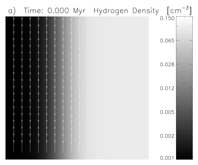
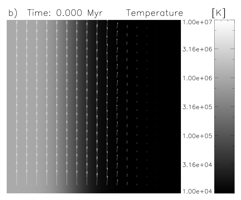
We start with warm gas, at a temperature of $T_{warm}=10^{4}~{}\rm{K}$, with a relatively high hydrogen number density $n_{warm}=0.1~{}\rm{cm^{-3}}$, and no mean motion, at the right side of the computational box. At the opposite side we have a low-density ($n_{hot}$), hot medium ($T_{hot}$), moving upward ($z$ direction) with a velocity $v_{hot}$. In some of our simulations we include a magnetic field $B_{z,warm}$ threading the warm gas aligned in the vertical direction, with a magnitude corresponding to a $\beta_{warm}\sim P_{gas}/P_{mag}\sim 1$. A sketch of the computational domain is presented in Figure 1.

Figure 1.— Schematic of the calculation cube, with hot gas moving upward on the left, and initially static warm gas to the right.

The two media are initially in total pressure equilibrium. The transition region (between hot and warm media) follows a hyperbolic tangent profile in the $x$ direction, that initially occupies $\sim 1/10$th. of the box size. The division line for the runs in a $144^{3}$ grid was set at the middle of the box. The vertical direction in all cases correspond to a physical scale of $L_{z}=10~{}\rm{pc}$. In the cases without cooling, the simulations can be rescaled arbitrarily, but when cooling is included the scale lengths are fixed by the value of the cooling rate used. The boundary conditions are periodic in the $z$ and $y$ directions. For the $x$ direction in the warm side of the box (right) we have a reflective boundary, and on the hot side (left) we have a source boundary condition. The latter reinforces the initial condition after each time-step, acting as a reservoir of hot material, that helps to balance the energy lost trough radiation. We initialized the computational cube with sinusoidal perturbations ($32$ harmonics, with random phases) in the component of the velocity normal to the interface of the two media ($v_{x}$). The shear at the boundary, will excite a K-H instability, which will eventually lead to the development of turbulence. A summary of the parameters we use is presented in Table 1.

Table 1 Parameters (initial conditions) of the runs used^a.

Modelb	$\log(T_{hot})$	$n_{hot}$	$v_{hot}$	$B_{z,warm}$	Grid size
	$[\rm{K}]$	$[\rm{cm^{-3}}]$	$[\rm{km~{}s^{-1}}]$	$[\mu\rm{G}]$
144-Th6-V50-B0	$6$	$1\times 10^{-3}$	$50$	$0$	$144^{3}$
144-Th6-V200-B0	$6$	$1\times 10^{-3}$	$200$	$0$	$144^{3}$
256-Th6-V200-B0	$6$	$1\times 10^{-3}$	$200$	$0$	$256^{3}$
LX-Th6-V200-B0	$6$	$1\times 10^{-3}$	$200$	$0$	$256\times 144^{2}$
144-Th7-V50-B0	$7$	$1\times 10^{-4}$	$50$	$0$	$144^{3}$
144-Th7-V200-B0	$7$	$1\times 10^{-4}$	$20$	$0$	$144^{3}$
144-Th6-V50-B1	$6$	$2\times 10^{-3}$	$50$	$\sim 2$	$144^{3}$
144-Th6-V200-B1	$6$	$2\times 10^{-3}$	$200$	$\sim 2$	$144^{3}$
144-Th7-V50-B1	$7$	$2\times 10^{-4}$	$50$	$\sim 2$	$144^{3}$
144-Th7-V200-B1	$7$	$2\times 10^{-4}$	$200$	$\sim 2$	$144^{3}$

4. Results

4.1. Evolution of the mixing layer

Our models, as described in the previous section, are dynamical and include a continuous transition between the hot and the warm media. In order to compare the result of our calculations with previous models of turbulent mixing layers (SSB93) we have to define what a region of “intermediate temperature” is, in our computational box. We adopted a threshold of $20\%$ departure from any of the nominal temperatures for the hot and warm media. That is, we consider in the transition region all material above $1.2\times 10^{4}~{}\rm{K}$, and below $8\times 10^{5}~{}\rm{K}$ for the runs where $T_{hot}=1\times 10^{6}~{}\rm{K}$; or bellow $8\times 10^{6}~{}\rm{K}$ for the runs with $T_{hot}=1\times 10^{7}~{}\rm{K}$. We evolve the initial conditions for $\sim$ 20,000 time-steps for all the cases with $144^{3}$ resolution. In Figures 2, and 3 we show the time evolution of all the purely hydrodynamical, and magnetized runs, respectively.

Figure 2.— Time evolution of the mixing layers, for the purely hydrodynamical runs. At the top (panel a) we present the density weighted average (thick lines), and volume average (thin lines) temperature of the mixing layers (material with a departure of $20\%$ from the nominal hot and warm temperatures). For reference we show the harmonic mean of the hot and warm temperatures (which corresponds to $\bar{T}$ in BF90, SSB93 with $\xi=1$ (dotted) horizontal lines, see eq.[1]). At the bottom (panel b) the mean hydrogen column density in the mixing layer (both panels are averages over different lines of sight normal to the layer –along the $x$ axis–).

Figure 3.— Same as Fig. 2, for the cases with magnetic field ($\beta\sim 1$) on the warm side.

We find in general, that the volume average temperature within the mixing layer depends strongly on the threshold used to define the intermediate temperature region. The density weighted temperature is more robust against the particular choice of threshold. And, since the emission observable is also density weighted, it is a better measure of the properties of mixing layers, and we will use it to interpret our results. Keeping in mind that the temperature in BF90 and SSB93 is a simple volume average, and that denser regions correspond to lower temperatures, our density weighted temperature will in general be lower. In our approach we do not assume a particular value for the efficiencies “$\eta$’s, and/or $\xi$” , instead they are being implicitly calculated. In principle they can be measured from the simulations, however, it would require the choice of an arbitrary temperature threshold to obtain a mean (volume average) temperature, which turns out to be very sensitive to such threshold. Thus, it is impractical to compare the models through estimates of the efficiencies

4.1.1 Formation of the mixing layer: early stages

Using a density weighted average, our calculations show a relatively cold boundary layer (of a few $10^{4}~{}\rm{K}$) at the early stages of formation. Due to the fact that the mass is initially on the warm side, this indicates a somewhat inefficient mixing at such early times.

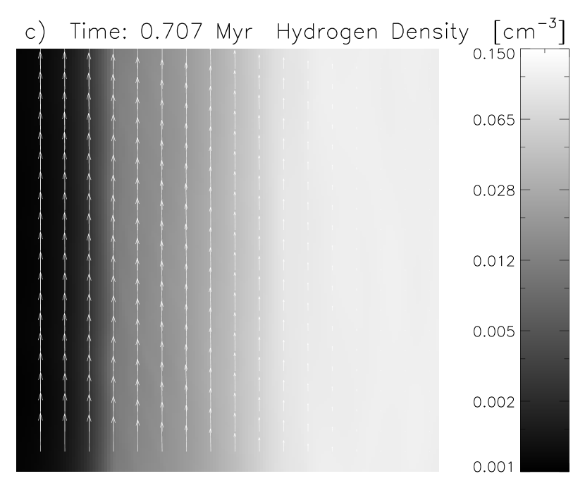
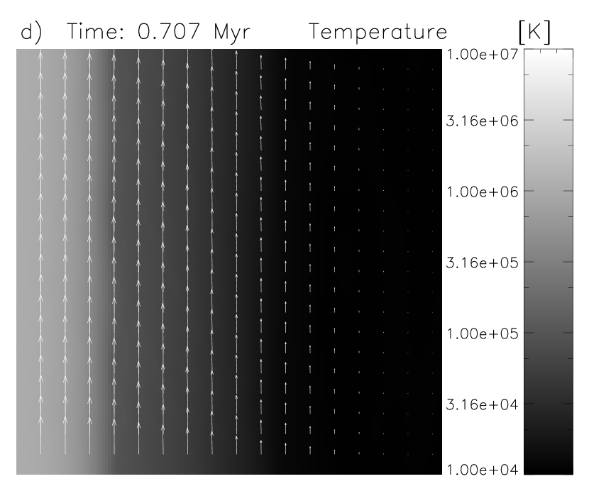
Figures 2b, and 3b show how the mixing layer develops. When we do not include cooling, the thickness of the boundary layer increases monotonically. The growth rate is faster when the shear velocity is larger, as expected for the K-H instability. For the cases in which cooling is included, we see a very different evolution, with the boundary layer shrinking with time at the beginning, and after some time starting to grow again. The smallest perturbations in the K-H instability have the fastest growth rate, but do not have the required energy to pull (enough) material into the mixing interface. Since the cooling is very effective, the transition layer is rather sharp. At this point, we mostly have warm gas being condensed at the interface, but mixing is not very effective yet. This is demonstrated in Figure 4, where we show cuts perpendicular to the mixing layer ($XZ$ plane) in two of our simulations after $t\sim 0.7~{}\rm{Myr}$.

Figure 4.— Selected snapshots of cuts in the $XZ$ plane from our simulations, showing density and temperature maps, along with the velocity field. The largest arrow in the velocity representation correspond to a magnitude of $\sim 200~{}\rm{km~{}s^{-1}}$ The upper two figures (panels a, b) correspond show the initial conditions for $v_{t}=200~{}\rm{km~{}s^{-1}}$, and $T_{hot}=10^{6}~{}\rm{K}$. In the middle (panels c, d) we show the evolution after $t\sim 0.7~{}\rm{Myr}$, without including cooling. At the bottom (panels e, f) we show the result after approximately the same time, but with the cooling included. We can see how the thickness of the mixing layer grows from the initial conditions where no cooling is present. At the same time, we can see the dramatic effect of cooling showing a rather sharp transition zone, and also how the largest wavelength modes of the K-H instability start to develop.

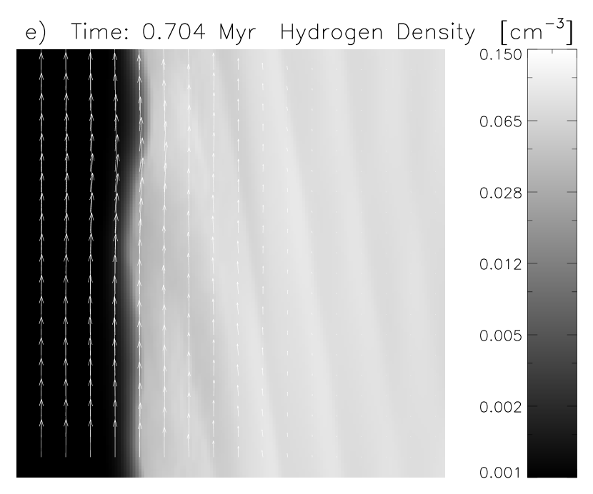
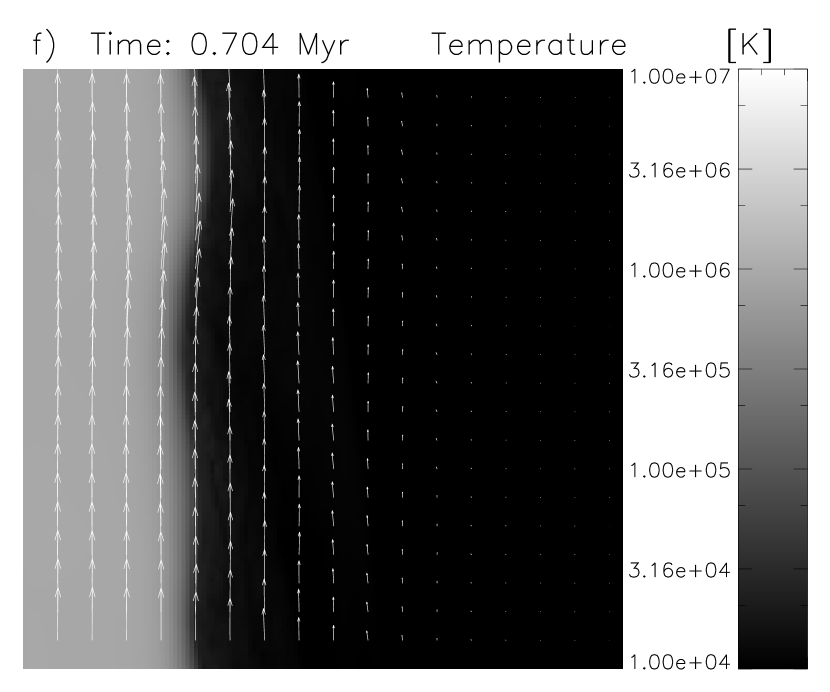
The cases with magnetic field do not show significant differences in the formation of the mixing layer when compared with the unmagnetized runs at early times ($t\lesssim 0.7$ Myr).

In order to test the sensitivity of our simulations to resolution we ran a couple of cases in a $256^{3}$ grid. The results are shown in Figure 5.

Figure 5.— Test of resolution convergence for a two set of simulations, one without cooling, and one with equilibrium cooling, both correspond to $T_{hot}=10^{6}~{}\rm{K}$ and $v_{t}=200~{}\rm{KM~{}s^{-1}}$. In panel a) we show the density weighted average temperature (thick lines), and the volume average temperature (thin lines). Panel b), shows the average H column density in the mixing layer.

We found marginal dependence on numerical resolution for the formation of the mixing layers. We will see however, that the mixing at later times is utterly dominated by the largest scales, when the modes that correspond to the longest wavelengths excited by the instability become apparent.

4.1.2 Evolution of the mixing layers at later times

Up until now, we have seen the formation of turbulent mixing layers by means of a K-H instability. However, we have not seen evidence of reaching a steady state, which is the original idea of the whole process. Since the largest modes in the K-H instability grow rather slowly, it is not practical to follow the evolution of all our models until steady state is achieved. Moreover, in a qualitative way, we have observed similar behavior for the runs that started with a larger temperature ($T_{hot}=10^{7}~{}\rm{K}$ ), but with the additional difficulty that we require finer time stepping for such cases, making it very difficult to cover a large span in time. To study the long-term evolution of the layer, we followed the the fastest evolving model. That is, the unmagnetized, $T_{hot}=10^{6}~{}\rm{K}$, and $v_{t}=200~{}\rm{km~{}s^{-1}}$ model. A related problem in our $144^{3}$ resolution runs was that by the time the mixing layer was reaching its asymptotic state (after $\sim 1.5~{}\rm{Myr}$), it was getting very close to the boundary of the computational box. To overcome this problem we extended the dimensions of the box to $256$ cells in the $x$ direction, and we placed the division between hot and warm media off-center. The new initial conditions (“LX-Th6-V200-B0” in Table 1) have only $1/4$th of the volume filled with warm gas, and the remainder with hot gas. This is because we have much more heat capacity in the warm gas (due to the density contrast), and because our simulations did not have enough hot gas to provide a steady state. Figure 6 illustrates the evolution of this extended model, which shows how the mixing layer broadens after the first signs of large modes of the instability appear (see Figures 4e and 4f).

Figure 6.— Further evolution of the runs corresponding to $T_{hot}=10^{6}~{}\rm{K}$, and $v_{z}=200~{}\rm{m~{}s^{-1}}$. The top panel (panel a) with the average temperature, (thin lines for volume average, and thick lines for the density weighted.) At the bottom (panel b) we see that for the case with equilibrium cooling, after the initial stage, the the mixing layer starts to grow.

We also show snapshots of cuts perpendicular to the layer, after $2.3~{}\rm{Myr}$ in Figure 7. This figure highlights how a fully operational K-H instability effectively mixes the two media and provides a much larger interface zone, compared with the times when only small scale modes are present.

Figure 7.— Snapshots of cuts in the $XZ$ plane for “NC-L2X-Th6-V200-B0.0” after $t\sim 2.3~{}\rm{Myr}$. Notice how the K-H instability has indeed produced turbulence at the boundary of the two media, increasing the thickness of the zone with intermediate temperatures ($T\sim 10^{5}~{}\rm{K}$).

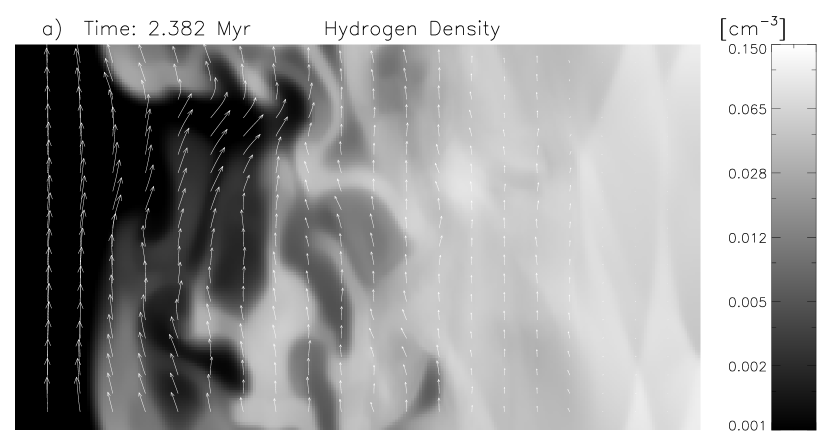
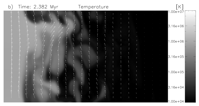
Even after $\sim 2.5~{}\rm{Myr}$, in the longer box ($256$ cells in the $x$ direction), the simulations have not reached a steady state. Nonetheless, our results provide important insights on how these mixing layers will develop and change over time.

4.2. Observational Diagnostics for Mixing Layers

Notably, the time evolution we observe for these mixing layers are associated with a significant evolution of spectral line diagnostics, most importantly the column densities and ratios of highly ionized species. These measurements depend not only on the metallicity, density contrast, and relative velocities of the mixing zones, but also on the evolutionary state of the layer. As a first step towards examining the evolution, we have calculated the column densities of C IV, N V, and O VI ions through our simulated layers as a function of time. Using the temperature and density profile along synthetic lines-of-sight (LOSs) through the data cube, chosen perpendicularly to the boundary layer (in the direction of the $x$ axis). These column densities were computed under the assumption of solar metallicity, and collisional ionization equilibrium (Benjamin et al., 2001). Figures 8 and 9 show the range of values of the C IV/O VI, and N V/O VI ratios along with other models of high ion production in the literature (compiled by Indebetouw & Shull 2004a, b). The central points are the mean C IV/O VI, and N V/O VI values averaged over all the possible LOSs, at a given point in time. The error bars were obtained at each time, with the dispersion of column densities for the various LOSs. The time domain was splitted evenly into $10$ bins from $t=0$ to the longest time available for each run (the final times can be checked in Figures 2, 3, and 6).

Figure 8.— Comparison of line ratios for various models in the literature, and our calculations (modified from Indebetouw & Shull (2004a, b). The triangles correspond to radiative cooling from a Galactic fountain model (Shapiro & Benjamin, 1993; Benjamin & Shapiro, 1993). The “x’s” are conductive heating and evaporation models of planar clouds (Boehringer & Hartquist, 1987; Borkowski, Balbus & Fristrom, 1990). Cooling of SNR shells are represented by “+’s” (Slavin & Cox, 1993; Shelton, 1998). The ion ratios in collisional ionization equilibrium from Sutherland & Dopita (1993) are in solid line (this corresponds to a range in temperatures, higher at the bottom center and lower at the upper right). SSB83 result for turbulent mixing layers are in asterisks. Our calculations are represented with circles, the color coding can be found in the legend of the plot. These last correspond to the average of LOSs normal to the boundary, for a given point in time each. The error bars were obtained considering the variability with the different LOSs.

Figure 9.— Same as Fig. 8, with our simulations that include magnetic field ($\beta\sim 1$).

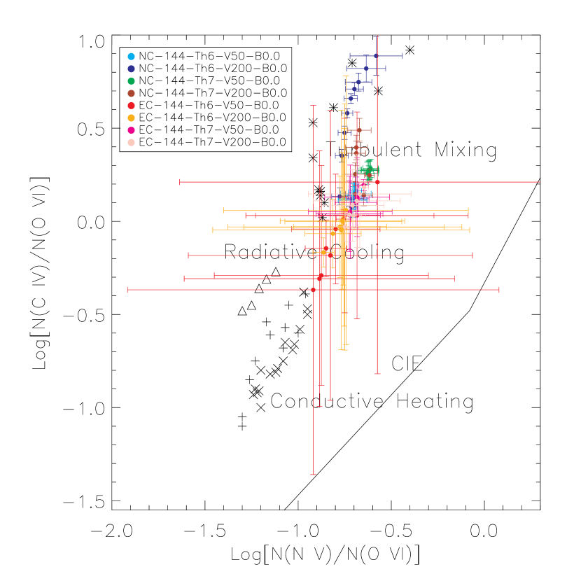
The line ratios and column densities from our simulations should not be interpreted too literally, but rather as a guide to obtain insight into the evolution of mixing layers. In particular, the assumption of collisional ion fraction equilibrium limits the accuracy of line ratios. As pointed out by SSB93, mixing layers can be quite far from equilibrium. The overall dynamics and time evolution of mixing layers is not likely to change dramatically by non-equilibrium effects. However, observational diagnostics such as line ratios can be affected significantly. A study of non-equilibrium cooling models with more emphasis on the observational implications is necessary and we plan to provide it in a following paper.

It is interesting that a clear difference is present between the runs that include cooling and those that do not. However, note that except for the “LX-Th6-V200” runs, the mixing layer is still in a very early stage of formation. It is remarkable that the models without cooling show similarity to the results of SSB93. Certainly their models did not account for the dynamical effect of the cooling: their model provides the intermediate temperatures, but the mixing is merely hydrodynamical. Condensation or evaporating flows were not considered. At the same time, their model also assumed fully developed turbulence, and our set of runs have not achieved the corresponding stationary state.

With new models, observations may be able to provide insights about the time-dependence of the mixing. Another thing to notice is the larger scatter for the cases that have been run for longer times. This scatter can be explained noting that for longer timescales we have a more dynamical (turbulent) picture, with many structures moving in and out of a particular LOS. Actually, the values of the C IV/O VI, N V/O VI ratios (and the rather large scatter), are somewhat consistent with the observations presented by Indebetouw & Shull (2004b). Is is also evident that in the magnetized cases the K-H instability (and therefore the development of turbulence at the boundary) is delayed. This can be seen from the smaller scatter of points in Figure 9 compared to those in 8. However, magnetic reconnection should not allow the magnetic field to form knots and prevent turbulent mixing motions (see Lazarian & Vishniac, 1999).

It remains difficult to reconcile the models with high ion column densities. It has been pointed out (e.g. SSB93; Savage et al. 2003; Indebetouw & Shull 2004a, b), that to explain the typical column densities observed,the LOS must pass through several mixing layers (sometimes as many as a hundred). Indeed, several interfaces are likely to be blended for long lines-of-sight (as in the case of observations in the halo of the galaxy). However, in many cases fairly smooth and symmetrical line profiles, with little centroid dispersions are observed. This evidence indicates that merely summing over a large number of interfaces may not explain the observed column densities. In Table 2 we present the column densities of an arbitrary artificial LOS after $0.7$ Myr for all the models with $T_{hot}=10^{6}~{}\rm{K}$. For comparison we include the values that correspond to the initial conditions.

Table 2Ion Column Densities^∗ at early times.

Model	C IV			N V			O VI
	$t=0$ Myr.	$t=0.7$ Myr.		$t=0$ Myr.	$t=0.7$ Myr.		$t=0$ Myr.	$t=0.7$ Myr.
NC-144-Th6-V50-B0.0	$12.03$	$12.06$		$11.19$	$11.20$		$11.89$	$11.90$
EC-144-Th6-V50-B0.0	$12.03$	$11.53$		$11.19$	$10.74$		$11.89$	$11.45$
NC-144-Th6-V200-B0.0	$12.03$	$12.34$		$11.19$	$11.05$		$11.89$	$11.79$
EC-144-Th6-V200-B0.0	$12.03$	$11.26$		$11.19$	$10.55$		$11.89$	$11.33$
NC-L2X-Th6-V200-B0.0	$12.03$	$12.36$		$11.20$	$11.06$		$11.93$	$11.83$
EC-L2X-Th6-V200-B0.0	$12.03$	$11.38$		$11.20$	$10.67$		$11.93$	$11.57$
NC-144-Th6-V50-B1.0	$12.29$	$12.34$		$11.47$	$11.51$		$12.18$	$12.22$
EC-144-Th6-V50-B1.0	$12.29$	$11.61$		$11.47$	$10.85$		$12.18$	$11.71$
NC-144-Th6-V200-B1.0	$12.29$	$12.84$		$11.47$	$11.65$		$12.18$	$12.06$
EC-144-Th6-V200-B1.0	$12.29$	$11.50$		$11.47$	$10.76$		$12.18$	$11.58$

In Figure 10 we show the mean column densities of C IV, N V, and O VI (for synthetic LOSs normal to the interface), as a function of time for the more evolved runs.

Figure 10.— Time evolution of the column density of different high ions for a line of sight perpendicular to the interface. The initial conditions correspond to $T_{hot}=10^{6}~{}\rm{K}$ and $v_{t}=200~{}\rm{km~{}s^{-1}}$.Thin lines correspond to the case without cooling, thick lines to equilibrium cooling.

Average values of column densities in the halo of the Galaxy observed with FUSE are (Savage et al., 2003; Indebetouw & Shull, 2004b): $\log N[$C IV$]\sim 14.3$, $\log N[$N V$]\sim 13.7$, and $\log N[$O VI$]\sim 14.5$. A survey with the Copernicus satellite in the Galactic plane by Jenkins (1978a, b), suggested that individual O VI components have column densities closer to $\log N[$O VI$]\sim 13$, which is similar to observations with FUSE of very nearby stars (Oegerle et al., 2005). The column densities obtained in the model that ran for the longest time (at $t\sim 2.5$ Myr), are slightly larger than those predicted by SSB93, but would still require too many interfaces to explain observations. However, as we have discused earlier, the simulations were stopped before fully reaching a stationary state, and the thickness of intermediate temperature zone was still increasing with time (see for instance Figure 6b). The results presented here suggest that not only the number of mixing layers, but the time available for turbulence to develop, are factors to consider for the proper interpretation of observations.

5. Summary

Turbulent mixing layers at the interfaces of the hot ($T\sim 10^{6-7}~{}\rm{K}$) and warm ($T\sim 10^{4}~{}\rm{K}$) media in the ISM can be produced by high shear, via a Kelvin-Helmholtz instability. We use a MHD code with radiative cooling, to model the formation and evolution of turbulent mixing layers through this instability.

The introduction of cooling in to the dynamical evolution was found to produce dramatic differences compared with the same models ran without cooling. For instance, the deposition of momenta from hot gas condensing onto the mixing layer modifies the growth-rate of the K-H instability, making it develop faster than the same case run without cooling.

The low density of the hot medium caused the growth rate of the large scale modes of the instability to be slow. At early stages of the formation of the mixing layer ($t~{}\lesssim 1~{}\rm{Myr}$) the rapid cooling of material at intermediate temperatures ($T\sim 10^{5}~{}\rm{K}$) makes for a sharp transition between the hot and warm media.

At later times, the instability excites large scale fluctuations that are powerful enough to provide more efficient mixing, and the transition zone broadens. We see evidence that for typical ISM conditions ($T_{hot}\sim 10^{6}~{}\rm{K}$ and $T_{warm}\sim 10^{4}~{}\rm{K}$, with a shear velocity of $200~{}\rm{km~{}s^{-1}}$), the mixing layer is still growing after $2.5\rm{Myr}$.

We included a dynamically important magnetic field ($\sim 2~{}\mu\rm{G}$) in the warm phase for some runs, and its effect was found to be minimal at earlier times $\lesssim 0.7$ Myr. At later times the magnetic field inhibits/delays the development of the K-H instability, and thus the turbulent mixing.

Assuming solar metallicities, and collisional ionization equilibrium fractions, we estimated column densities and line ratios of highly ionized species (C IV, N V, and O VI) from our simulations. We compared our results with previous models (SSB93) of turbulent mixing layers and found similar column densities. The C IV/O VI, and N V/O VI mean line ratios are slightly different, with a lower C IV/O VI. We also found a significant scatter between different lines-of-sight, in particular for the models evolved to longer times.

We were not able to fully reach a stationary state in our simulations, however our results suggest that given more time ($\gtrsim 2.5~{}\rm{Myr}$ for typical conditions), the column density of high ions should be significantly larger than previous models, partially alleviating the problem of number of layers required to explain observations.

References

- Begelman & Fabian (1990) Begelman, M. C., & Fabian, A. C. 1990, MNRAS, 244, 26P (BF90)
- Benjamin & Shapiro (1993) Benjamin, R. A., & Shapiro, P. 1993, in Ultraviolet and X-Ray Spectroscopy of Laboratory and Astrophysical Plasmas, ed. E. H. Silver & S. M. Kahn (New York: Cambridge Univ. Press), 280
- Cho & Lazarian (2002) Cho, J. & Lazarian, A. 2002, Phys. Rev. Lett., 88, 245001
- Cho et al. (2003) Cho, J., Lazarian, A., Honein, A., Knaepen, B., Kassinos, S., Moin, P. 2004, ApJ, 589, L77
- Cox (2005) Cox, D.P. 2005, ARAA, in press
- Benjamin et al. (2001) Benjamin, R. A., Benson, B. A., & Cox, D. P. 2001, ApJ, 554, L225
- Boehringer & Hartquist (1987) Boehringer, H., & Hartquist, T. W. 1987, MNRAS, 228, 915
- Borkowski et al. (1990) Borkowski, K. J., Balbus, S. A., & Fristrom, C. C. 1990, ApJ, 355, 501
- Brio & Wu (1988) Brio, M., & Wu, C.C. 1988, Jour. of Comp. Phys., 75, 500
- Chandrasekhar (1961) Chandrasekhar, S. 1961, Hydrodynamic and Hydromagnetic Stability (New York: Oxford Univ. Press)
- Frank et al. (1996) Frank, A., Jones, T. W., Ryu, D., & Gaalaas, J. B. 1996, ApJ, 460, 777
- Gamie et al. (2003) Gammie, C., McKinney, J., & Tóth, G. 2003, ApJ, 589, 444
- Harten et al. (1983) Harten, A., Lax, P., & van Leer, B. 1983, SIAM Rev., 25, 35
- Indebetouw & Shull (2004a) Indebetouw, R., & Shull, J. M. 2004a, ApJ, 605, 205
- Indebetouw & Shull (2004b) Indebetouw, R., & Shull, J. M. 2004b, ApJ, 607, 309
- Jenkins (1978a) Jenkins, E. B. 1978a, ApJ, 219, 845
- Jenkins (1978b) Jenkins, E. B. 1978b, ApJ, 220, 107
- Koyama & Inutsuka (2004) Koyama, H., & Inutsuka, S.-i. 2004, ApJ, 602, L25
- Kurganov et al. (2001) Kurganov, A., Noelle, S., & Petrova G. 2001,SIAM J. Sci. Comput., 23, 707
- Lazarian (2006) Lazarian, A. 2006, ApJ, submitted
- Lazarian & Vishniac (1999) Lazarian, A., Vishniac, E. T. 1999, ApJ, 517, 700
- Narayan & Medvedev (2001) Narayan, R., Medvedev, M. V. 2001, ApJ, 562, L129
- Oegerle et al. (2005) Oegerle, W.R, Jenkins, E. B., Shelton, R. L., Bowen, D. V., Chayer, P. 2005, ApJ, 622, 377
- Ryu & Jones (1995) Ryu, D. & Jones, T.W. 1995, ApJ, 442, 228
- Ryu et al. (2000) Ryu, D., Jones, T. W., Frank, A. 2000, ApJ, 545, 475
- Savage et al. (2003) Savage, B. D., et al. 2003, ApJS, 146, 125
- Shapiro & Benjamin (1993) Shapiro, P. R., & Benjamin, R. A. 1993, in Star Formation, Galaxies and the Interstellar Medium, ed. J. Franco, F. Ferrini, & G. Tenorio-Tagle (New York: Cambridge Univ. Press), 275
- Shelton (1998) Shelton, R. L. 1998, ApJ, 504, 785
- Slavin & Cox (1993) Slavin, J. D., & Cox, D. P. 1993, ApJ, 417, 187
- Slavin et al. (1993) Slavin, J. D., Shull, J. M., & Begelman, M. C. 1993, ApJ, 407, 83 (SSB93)
- Sutherland & Dopita (1993) Sutherland, R. S., & Dopita, M. A. 1993, ApJS, 88, 253
- Tóth (2000) Tóth, G. 2000, Jour. of Comp. Phys., 161, 605
- Wakker & van Woerden (1997) Wakker, B. P.,& van Woerden, H. 1997, ARA&A, 35, 217