How accurate are the time delay estimates
in gravitational lensing?

We present a novel approach to estimate the time delay between light curves of multiple images in a gravitationally lensed system, based on Kernel methods in the context of machine learning. We perform various experiments with artificially generated irregularly-sampled data sets to study the effect of the various levels of noise and the presence of gaps of various size in the monitoring data. We compare the performance of our method with various other popular methods of estimating the time delay and conclude, from experiments with artificial data, that our method is least vulnerable to missing data and irregular sampling, within reasonable bounds of Gaussian noise. Thereafter, we use our method to determine the time delays between the two images of quasar Q0957+561 from radio monitoring data at 4 cm and 6 cm, and conclude that if only the observations at epochs common to both wavelengths are used, the time delay gives consistent estimates, which can be combined to yield $408\pm 12$ days. The full 6 cm dataset, which covers a longer monitoring period, yields a value which is 10% larger, but this can be attributed to differences in sampling and missing data.

1 Introduction

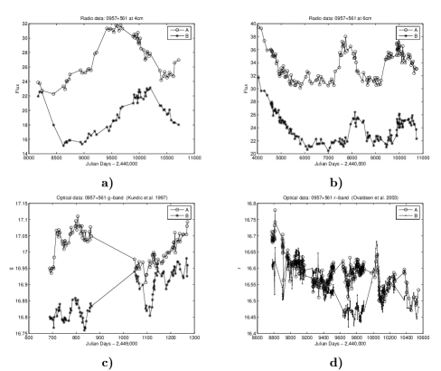
Long before the first gravitationally lensed quasar was discovered in 1979 (Walsh et al. 1979), Refsdal suggested that time delays of source fluctuations between the multiple images could be used to measure the Universe (Refsdal 1964, 1966). This first lensed quasar, Q0957+561, is also the most studied so far (Fig. 1), and many attempts have been made to estimate the time delay between its two principal images.

The measurement of the delay between the images A and B of Q0957+561 has been the subject of sensitive controversy ever since the first claim of measurement in the early 1980s. Haarsma et al. (1997) reviews the various measurements, showing how various delays in the range of 300 to 1000 days have been claimed, from various data sets using different methods (Kochanek & Schechter 2004). In the early nineties, the quoted time delay values were either around 420 days (e.g., Falco et al. 1991) or 540 days (e.g., Press et al. 1992), culminating in a “definitive” measure of a time delay of 417$\pm$3 days (Kundic et al. 1997).

More recently, efforts have concentrated on characterising the errors on such measurements (e.g., Pindor 2005). The case of Q0957+561 also illustrates this. Variously, from optical monitoring data, Ovaldsen et al. (2003), Oscoz et al. (2001), Burud et al. (2001) and Colley et al. (2003) estimate a time delay of 424.9$\pm$1.2 422.6$\pm$0.6, 423$\pm$9 and 417$\pm$0.07 days respectively (more estimates are in Table 1). Given the error bars, many of these measures are inconsistent with the definitive value quoted above, and often with each other, if taken at face value.

To measure the time delay between signals arriving from the same source but via different paths, typically ranging from a few days to a few years in the data available so far, one needs to frequently observe the same set of sources over long periods of time. Due to the usual methods of allocation of telescope time and the natural time scale of projects, the data obtained typically are not regularly sampled, and could be obtained by a wide range of instruments and at different frequencies, often with large gaps in the time series. Since the use of time delays in constraining cosmological parameters (e.g., Saha 2004) requires these delays to be measured to a precision and reliability that is better than afforded by current practice, it is important to look for better and more robust methods, where the dependence of the results on the incompleteness of the data is well understood.

Rigorous error estimates based on a functional form for random errors often well represent the inherent limitations of a particular method, but do not address systematic effects due to sampling strategies, to the heterogeneity of monitoring programmes and those due to data missing for various practical reasons, like observing schedules. With the bank of data for light curves of lens systems growing rapidly, the effect of such systematics on the measured values of time delay need to be well understood. This is particularly important in view of future missions like the Large Synoptic Survey Telescope (LSST) and Supernova/Acceleration Probe (SNAP), which will make large monitoring data sets available for hundreds of multiply-imaged distant sources, (e.g., Mörtsell et al. 2005; Fassnacht et al. 2004), thus rendering them major statistical tools for cosmological purposes.

We present a novel approach to the problem of determining the delay between noisy time-dependent signals that have been measured at irregular intervals over several years, often with large gaps in the monitoring programme. Ours is an automatic method that allows us to analyse large-scale experiments more accurately than typical methods. We study the effect of gaps of various length, regularly or irregularly sampled, in the monitoring data, in addition to the different levels of noise. This study should provide some insight for astronomers designing future observational campaigns for monitoring multiple-images quasars.

As an illustration of the application of our method, we apply it here to radio observations, at 4 cm and 6 cm, of the well known gravitational lens Q0957+561 (Haarsma et al. 1999), and compare the results to other studies using the same or similar datasets.

The remainder of this article is organised as follows: in §2, we present our method. §3 is a survey of methods to estimate the time delay presenting a detailed review of three of the most popular methods. §4 describes the artificial data generated to perform our simulations. §5 shows the results on these artificial data. In §7 we present estimates for the time delay between the two principal images of Q0957+561 from radio data at 4 cm and 6 cm, using our methods presented here, followed by a concluding summary.

2 The model

We model the observed flux at a given frequency (in the radio or optical range) from two lensed images A and B of the same distant source, as two time series

$$x_{A}(t_{i})=h_{A}(t_{i})+\varepsilon_{A}(t_{i})\\ x_{B}(t_{i})=M\cdot h_{B}(t_{i})+\varepsilon_{B}(t_{i}),$$ (1)

where $M$ is the ratio of the fluxes of the two images, and $t_{i},i=1,2,...,n$ are discrete observation times. The observation errors $\varepsilon_{A}(t_{i})$ and $\varepsilon_{B}(t_{i})$ are modelled as zero-mean Normal distributions

$$N(0,\sigma_{A}(t_{i}))\ \ \hbox{and}\ \ N(0,\sigma_{B}(t_{i})),$$ (2)

respectively. Now,

$$h_{A}(t_{i})=\sum_{j=1}^{N}\alpha_{j}K(c_{j},t_{i})$$ (3)

is the “underlying” light curve that underpins image A, whereas

$$h_{B}(t_{i})=\sum_{j=1}^{N}\alpha_{j}K(c_{j}+\Delta,t_{i})$$ (4)

is a time-delayed (by $\Delta$) version of $h_{A}(t_{i})$ underpinning image B.

The functions $h_{A}$ and $h_{B}$ are formulated within the generalised linear regression framework (e.g. Shawe-Taylor & Cristianini 2004, §2). Each function is a linear superposition of $N$ kernels $K(\cdot,\cdot)$ centred at either $c_{j}$, $j=1,2,...,N$ (function $f_{A}$), or $c_{j}+\Delta$, $j=1,2,...,N$ (function $f_{B}$). The model (1)-(4) has $N$ free parameters $\alpha_{j}$, $j=1,2,...,N$, that need to be determined by (learned from) the data. We use Gaussian kernels of width $\omega^{2}$:  for $c,t\in\Re$,

$$K(c,t)=\exp\,{\frac{-|t-c|^{2}}{\omega_{c}^{2}}}.$$ (5)

The kernel width $\omega_{c}>0$ determines the ‘degree of smoothness’ of the underlying curves $h_{A}$ and $h_{B}$. We describe setting of $\omega_{j}=\omega_{c_{j}}$ and regression weights $\alpha_{j}$ in the next subsections. In this study, we position kernels on all observations, i.e. $N=n$.

Finally, our aim is to estimate the time delay $\Delta$ between the temporal light curves corresponding to images A and B. Given the observed data, the likelihood of our model reads

$$P({\rm Data}\ |\ {\rm Model})=\prod_{i=1}^{n}p(x_{A}(t_{i}),x_{B}(t_{i})\ |\ \Delta,\{\alpha_{j}\}),$$ (6)

where

$$p(x_{A}(t_{i}),x_{B}(t_{i})\ |\ \Delta,\{\alpha_{j}\}) = \frac{1}{2\pi\sigma_{A}^{2}(t_{i})\sigma_{B}^{2}(t_{i})}$$ (7)

$$\exp\left\{\frac{(x_{A}(t_{i})-h_{A}(t_{i}))^{2}}{2\sigma_{A}^{2}(t_{i})}\right\}$$

$$\exp\left\{\frac{(x_{B}(t_{i})-M\cdot h_{B}(t_{i}))^{2}}{2\sigma_{B}^{2}(t_{i})}\right\}.$$

The negative log-likelihood (without constant terms) simplifies to

$$Q=\sum_{i=1}^{n}\left(\frac{(x_{A}(t_{i})-h_{A}(t_{i}))^{2}}{\sigma_{A}^{2}(t_{i})}+\frac{(x_{B}(t_{i})-M\cdot h_{B}(t_{i}))^{2}}{\sigma_{B}^{2}(t_{i})}\right).$$ (8)

To avoid extrapolation when we apply a time delay to our underlying curve, we do not evaluate the goodness of fit over all observations:

$$Q=\sum_{u=1}^{n-b_{1}}\frac{(x_{A}(t_{u})-h_{A}(t_{u}))^{2}}{\sigma_{A}^{2}(t_{u})}+\sum_{v=b_{2}}^{n}\frac{(x_{B}(t_{v})-M\cdot h_{B}(t_{v}))^{2}}{\sigma_{B}^{2}(t_{v})},$$ (9)

where $b_{1}$ is the greatest index satisfying $t_{n-b_{1}}\leq t_{n}-\Delta_{max}$, and $b_{2}$ is the smallest index satisfying $t_{b_{2}}\geq t_{1}+\Delta_{max}$. Here, $\Delta_{max}$ is the maximum possible time delay we are willing to consider (fixed).

We determine the model parameters and evaluate Eq. (9) for a series of trial values of $\Delta$. The time delay is then estimated as the value of $\Delta$ with minimal cost (9). Note that if the errors cannot be modelled as Gaussian, Eq. (9) would need to be rewritten using an appropriate noise term.

2.1 Weights

We rewrite Eq. (8) as

$$Q=\sum_{i=1}^{n}\left(\left[\frac{x_{A}(t_{i})}{\sigma_{A}(t_{i})}-\frac{h_{A}(t_{i})}{\sigma_{A}(t_{i})}\right]^{2}+\left[\frac{x_{B}(t_{i})}{\sigma_{B}(t_{i})}-\frac{M\cdot h_{B}(t_{i})}{\sigma_{B}(t_{i})}\right]^{2}\right).$$ (10)

Since we expect each of the two terms in (10) to be individually equal to zero, we impose

$$\@vec{K}\@vec{\alpha}=\@vec{x},$$ (11)

where $\@vec{\alpha}=(\alpha_{1},\alpha_{2},...,\alpha_{N})^{T}$,

$$\@vec{K}=\left[\begin{array}[]{ccc}K_{A}(c_{1},t_{1})&\cdots&K_{A}(c_{N},t_{1})\\ \vdots&\ddots&\vdots\\ K_{A}(c_{1},t_{n})&\cdots&K_{A}(c_{N},t_{n})\\ \hline\cr K_{B}(c_{1},t_{1})&\cdots&K_{B}(c_{N},t_{1})\\ \vdots&\ddots&\vdots\\ K_{B}(c_{1},t_{n})&\cdots&K_{B}(c_{N},t_{n})\end{array}\right],\ \ \ \ \ \ \ \ \@vec{x}=\left[\begin{array}[]{c}\frac{x_{A}(t_{1})}{\sigma_{A}(t_{1})}\\ \vdots\\ \frac{x_{A}(t_{n})}{\sigma_{A}(t_{n})}\\ \hline\cr\frac{x_{B}(t_{1})}{\sigma_{B}(t_{1})}\\ \vdots\\ \frac{x_{B}(t_{n})}{\sigma_{B}(t_{n})}\end{array}\right],$$ (12)

and the kernels $K_{A}(\cdot,\cdot)$, $K_{B}(\cdot,\cdot)$ have the form:

$$K_{A}(c,t)=\frac{K(c,t)}{\sigma_{A}(t)},\ \ \ \ \ \ \ K_{B}(c,t)=\frac{M\cdot K(c+\Delta,t)}{\sigma_{B}(t)}.$$ (13)

Hence,

$$\@vec{\alpha}=\@vec{K}^{+}\@vec{x}.$$ (14)

We regularise the inversion in (14) through singular value decomposition (SVD).

2.2 Kernel parameters

In general, in order to use Gaussian kernels (5) in generalised linear regression (1)-(4), the kernel positions $c_{j}$, as well as kernel widths $\omega_{j}$, need to be determined (Shawe-Taylor & Cristianini 2004, §9). Several approaches have been taken in the literature. For instance, those who use radial basis function (RBF) networks employ e.g. $k$-means clustering, or EM algorithm and Gaussian mixture modelling (e.g. see Haykin 1999; Hastie et al. 2001). We have explored two approaches to kernel positioning: (i) the centres $c_{j}$ uniformly distributed across the input range and (ii) the centres $c_{j}$ positioned at input samples $t_{j}$, $j=1,2,...,n$. The latter approach lead to superior performance and the results reported in this paper were obtained using kernels centred at observation times $t_{j}$. As for the kernel widths, we propose two approaches: (j) fixed width $\omega$ and (jj) variable widths $\omega_{j}$, $j=1,2,...,n$. Both are described in the following subsections.

2.2.1 Fixed kernel width

The width of the kernels determines the degree of smoothing for the underlying flux curves (3) and (4). Finding ‘appropriate’ values of smoothing parameters is one of the challenges in non- and semi-parametric regression. We use cross validation (Hastie et al. 2001, §7.10) to find the ‘optimal’ kernel width $\omega$. In particular, we invoke a variant of five-fold-cross-validation. We start by dividing the data set uniformly into five blocks. In the first step, we construct a validation set as a collection of the first elements of each block. The validation set has five elements. The training set is formed by the remaining observations, i.e. the observations not included in the validation set. We fit our models on the training set and determine the mean square error (MSE) over a range of delay values $\Delta$ on the validation set. In the next step, we construct a new validation set as a collection of the second elements of each block. The new training set is again formed by the remaining observations. As before we fit our models on the training set and determine MSE on the validation set. We repeat this procedure $r$ times, where $r$ is the number of observations in each block. Finally, the mean of all such mean square errors (there is $r$ of them), MSE_CV, is calculated. The kernel width $\omega$ selected using the cross-validation is the kernel width yielding the smallest MSE_CV. The scheme is summarised in Algorithm 1.

Fix $M$, $LowerBound$ and $UpperBound$

Fix $Blocks\leftarrow 5$

Fix $PointsPerBlock\leftarrow min(\{b_{1},n-b_{2}\})/Blocks$

for $omega\leftarrow LowerBound$ to $UpperBound$ do  for $i\leftarrow 1$ to $PointsPerBlock$ do  Remove the $i^{th}$ observation of each block and include it in the validation set

for $\Delta\leftarrow\Delta_{min}$ to $\Delta_{max}$ do  Get weights $\@vec{\alpha}$ on the training set (using eq. (14))

Compute $h_{A}(t_{u})$ and $h_{B}(t_{v})$

Get MSE on the validation set

$S(\Delta)\leftarrow$MSE

  $R(i)\leftarrow mean(S)$   $Best(omega)\leftarrow mean(R)$   $\omega\leftarrow\arg\!\min_{\omega}(Best)$

Algorithm 1 Cross validation

2.2.2 Variable kernel width

Rather than considering a fixed kernel width $\omega$, in this section we allow variable width Gaussian kernels of the form

$$K(c_{j},t_{i})=\exp{\frac{-|t_{i}-c_{j}|^{2}}{\omega_{j}^{2}}}\;;\;K(c_{j}+\Delta,t_{i})=\exp{\frac{-|t_{i}-(c_{j}+\Delta)|^{2}}{\omega_{j}^{2}}}.$$

We determine each $\omega_{j}$ through a smoothing parameter $k\in\{1,2,...,k_{max}\}$. Parameter $k$ is the number of neighbouring observations $t_{i}$ on both sides of $c_{j}$ (boundary conditions need to be taken into account). In particular, since we centre a kernel on each observation time, i.e. $c_{j}=t_{j}$, we have the cumulative kernel width

$$\omega_{j}=\sum_{d=1}^{k}(t_{j}-t_{j-d})+(t_{j+d}-t_{j})=\sum_{d=1}^{k}(t_{j+d}-t_{j-d}).$$ (15)

The optimal value of $k$ can be estimated using a cross-validation procedure analogous to that of section §2.2.1.

Figure 1: The variation of flux density with time of the two gravitationally lensed images of Quasar Q0957+561. a) Radio data at 4 cm, b) radio data at 6 cm (Haarsma et al. 1999), c) optical data at g-band (Kundic et al. 1997), and d) optical data at r-band (Ovaldsen et al. 2003).

3 Methods for estimating the Time delay

Table 1 contains a review, in chronological order, of the more recent time delay estimates of the quasar Q0957+561 and the methods employed. This gravitational lens is the most extensively monitored so far, being the first one to be discovered. Fig. 1 presents examples of the observed light curves across various frequency bands, from radio to optical. As is evident in Table 1, whole range of time delay estimates (with varying uncertainty bounds) for the gravitational lens are available. The problem is that we do not know the actual time delay. One of the aims of this paper is to study the reliability of several time delay estimation methods in a large set of controlled experiments on artificially generated data with realistically modelled observational noise and mechanisms of missing measurements. We feel that only after learning lessons from such a study does it make sense to come up with yet another batch of time delay estimation claims.

Table 1: Review of time delay estimates between the two images of Q0957+561 from 1997 to 2004. The methods are reviewed in §3.

Reference	Method(s)	Time delay
Kundic et al. 1997	- Linear	417$\pm$3
	- Cross correlation
	- PRH
	- Dispersion
Oscoz et al. 1997	- Cross correlation	427$\pm$3
	- Dispersion
Pijpers 1997	- SOLA	425$\pm$17
Pelt et al. 1998b	- Dispersion	416.3$\pm$1.7
Haarsma et al. 1999	- PRH	409$\pm$30
	- Dispersion
Oscoz et al. 2001	- Linear	422.6$\pm$0.6
	- Cross correlation
	- Dispersion
Burud et al. 2001	- $\chi^{2}$ algorithm	423$\pm$9
Colley et al. 2003	- PRH	417.09$\pm$0.07
Ovaldsen et al. 2003	- Dispersion	424.9$\pm$1.2
	- $\chi^{2}$ algorithm

In this section, we review the principal time delay estimation methods that have been used on gravitational lens data. The Cross correlation method (Kundic et al. 1997; Oscoz et al. 1997), PRH method (Press et al. 1992) and Dispersion spectra, (Pelt et al. 1996), described in §3.1, §3.2 and 3.3, respectively, have been widely used in the literature. We employ them in §5 as base-line models when reporting performance of our methods (described in §2).

Of the methods mentioned in Table 1, the Linear method uses chi-squared ($\chi^{2}$) fitting (Press et al. 1986, §14). Since the data are irregularly sampled, linear interpolation in the observational gaps is performed (Kundic et al. 1997).

The method of Subtractive Optimally Localised Averages (SOLA) has been proposed as a method for solving inverse problems. The method was adopted by Pijpers (1997) who formulated time delay estimation as an inverse problem. It is worth nothing that SOLA employs kernels, called averaging kernels. However, SOLA differs from our approach in several respects: (i) SOLA does a symmetric treatment of the two estimated fluxes (flux A is fixed and flux B is varied to match A and vice versa), (ii) the reported time delay is the mean of the estimated time delays in the two symmetric cases, (iii) a free parameter is used to adjust the relative weighting of the errors in the variance-covariance matrix. We also note that parameter estimation in SOLA is problematic (Larsen & Hansen 1997; Rabello-Soares et al. 1999) and this method has been rarely used.

The $\chi^{2}$ algorithm (Burud et al. 2001; Ovaldsen et al. 2003) is a $\chi^{2}$-based method similar in spirit to our model in that it also uses a notion of an underlying model curve when fitting the two observed fluxes. However, the underlying model is assumed to be regularly sampled. It is regularised using a smoothing term (Burud et al. 2001, Eq. 3). Confidence intervals on the delay are estimated by performing Monte Carlo simulations (Burud et al. 2001).

In general, when Monte Carlo simulations are not performed, bootstrap techniques are used to calculate uncertainty in time delay estimates.

3.1 Cross correlation

Basically, there are two versions of methods based on cross correlation: the Discrete Correlation Function (DCF) and its variant, the Locally Normalised Discrete Correlation Function (LNDCF). Both calculate correlations directly on discrete pairs of light curves (Edelson & Krolik 1988; Lehar et al. 1992). These methods avoid interpolation in the observational gaps. Also, they are the simplest and fastest time delay estimation methods.

First, time differences (lags), $\Delta t_{ij}=|t_{j}-t_{i}|$, between all pairs of observations are binned into discrete bins. Given a bin size $\Delta\tau$, the bin centred at lag $\tau$ is the time interval $[\tau-\Delta\tau/2,\tau+\Delta\tau/2]$. $P(\tau)$ is the number of observational pairs in the bin centred at $\tau$. The DCF at lag $\tau$ is given by

$$DCF(\tau)=\frac{1}{P(\tau)}\sum_{i,j}\frac{(x_{A}(t_{i})-\bar{a})(x_{B}(t_{j})-\bar{b})}{\sqrt{(\sigma_{a}^{2}-\sigma_{A}^{2}(t_{i}))(\sigma_{b}^{2}-\sigma_{B}^{2}(t_{j}))}},$$ (16)

where $\bar{a}$ and $\bar{b}$ are means of the observed data fluxes $x_{A}(t_{i})$ and $x_{B}(t_{j})$, respectively; $\sigma_{a}^{2}$ and $\sigma_{b}^{2}$ are their variances; $\sigma_{A}^{2}(t_{i})$ and $\sigma_{B}^{2}(t_{j})$ are the observational errors (2).

Likewise,

$$LNDCF(\tau)=\frac{1}{P(\tau)}\sum_{i,j}\frac{(x_{A}(t_{i})-\bar{a}(\tau))(x_{B}(t_{j})-\bar{b}(\tau))}{\sqrt{(\sigma^{2}_{a}(\tau)-\sigma_{A}^{2}(t_{i}))(\sigma^{2}_{b}(\tau)-\sigma_{B}^{2}(t_{j}))}},$$ (17)

where $\bar{a}(\tau)$, $\bar{b}(\tau)$, $\sigma^{2}_{a}(\tau)$ and $\sigma^{2}_{b}(\tau)$ are the lag means and variances in the bin centred at $\tau$. The time delay is found when $DCF(\tau)$ and $LNDCF(\tau)$ (16)-(17) are maximum, i.e. at the best correlation.

3.2 The PRH method

This method is widely used for time delay estimation. Its fundamentals are based on the theory of stochastic processes and Wiener filtering (Press et al. 1992; Rybicki & Press 1992). Given two light curves $x_{A}$ and $x_{B}$ (1), the PRH method combines them into a single series $\@vec{y}$ by assuming a time delay $\Delta$ and a constant ratio $M$ between $x_{A}$ and $x_{B}$. Thus, for each of the two fluxes, we end up having a new data set of $2n$ observations; half is interpolated using the other flux. The flux ratio $M$ is estimated as a difference between weighted means of the fluxes; the weights are derived from the quoted observational errors. The time delay, $\Delta$, is estimated by minimising

$$\chi^{2}=\@vec{y\/}^{\rm T}\left(\@vec{A}-\frac{\@vec{A}\@vec{E}\@vec{E\/}^{\rm T}\@vec{A}}{\@vec{E\/}^{\rm T}\@vec{A}\@vec{E}}\right)\@vec{y},$$ (18)

which is a measure of goodness of fit on measurements from a Gaussian process (Press et al. 1992). Here, $\@vec{y}$ is the combined flux, $\@vec{E}$ is a column vector of ones, and

$$\@vec{A}=\@vec{B}^{-1}\equiv\left\{C_{ab}+\langle\sigma_{a}^{2}\rangle\delta_{ab}\right\}^{-1}$$ (19)

where

$$C_{ab}=\langle y(t_{a})y(t_{b})\rangle\equiv C(t_{a}-t_{b})\equiv C(\tau)$$ (20)

is a covariance model estimated from the data; $t_{a}$, $t_{b}$, $a,b=1,...,2n$, are sample times of the combined light curve. Press et al. (1992) suggest finding $C(\tau)$ through a first-order structure function $V(\tau)=\langle s^{2}\rangle-C(\tau)$, where $s$ is the clean data from $\@vec{y}$. Then, the structure function $V(\tau)$ is computed from the data, single image, by determining lags

$$\tau_{ij}\equiv|t_{i}-t_{j}|$$ (21)

and values

$$v_{ij}\equiv(x_{\{A,B\}}(t_{i})-x_{\{A,B\}}(t_{j}))^{2}-\sigma_{\{A,B\}}^{2}(t_{i})-\sigma_{\{A,B\}}^{2}(t_{j}).$$ (22)

where $\{A,B\}$ denotes that it comes from either image A or image B (1)-(2).

All pairs ($\tau_{ij}$, $v_{ij}$) are sorted with respect $\tau_{ij}$ and binned into 100 bins (Press et al. 1992, pg. 407). The values of $\tau_{ij}$ and $v_{ij}$ in each bin are averaged and finally a power-law model is built to fit the binned list,

$$V(\tau)=c_{1}\tau^{c_{2}}.$$ (23)

Note that this model is linear in log scale,

$$V(\ln(\tau))=\ln(c_{1})+{c_{2}}\ln(\tau).$$ (24)

Parameters $c_{1}$ and $c_{2}$ of the structure function can be determined using a simple line fitting algorithm. So, $V(\tau)$ is estimated on a single flow and one would naturally expect that estimates of $V(\tau)$ on flux $A$ would be similar to those on flux $B$. However, this is often not the case. Press et al. (1992) claim that it does not matter which image is chosen for the $V(\tau)$ estimation as the time delay calculations are sufficiently robust to variations in the $V(\tau)$ estimates. Our experience suggests that this may be an overoptimistic expectation. Moreover, the matrix $\@vec{B}$ (19) is often ill conditioned and we regularise the inversion operation through SVD.

3.3 Dispersion spectra

Dispersion is a weighted sum of squared differences between $x_{A}(t_{i})$ and $x_{B}(t_{i})$ (Pelt et al. 1996, 1998b, 1998a, 2002). The method is similar to those based on DCF (see §3.1). However, it models the time series of two light curves in a different way by combing them (given a time delay $\Delta$ and ratio $M$) into a single flux flow, $\@vec{y}$, as in the PRH method (§3.2). We worked with two versions of this method (see Pelt et al. 1998b):

$$D_{1}^{2}(\Delta)=\!\min_{M}\frac{\sum_{a=1}^{2n-1}w_{a}\left(y(t_{a+1})-y(t_{a})\right)^{2}}{2\sum_{a=1}^{2n-1}w_{a}}$$ (25)

and

$$D_{4,2}^{2}(\Delta)=\!\min_{M}\frac{\sum_{a=1}^{2n-1}\sum_{c=a+1}^{2n}S_{a,c}^{(2)}W_{a,c}G_{a,c}\left(y(t_{a})-y(t_{c})\right)^{2}}{2\sum_{a=1}^{2n-1}\sum_{c=a+1}^{2n}S_{a,c}^{(2)}W_{a,c}G_{a,c}},$$ (26)

where

$$w_{a}=\frac{1}{\sigma^{2}(t_{a+1})+\sigma^{2}(t_{a})},\\ W_{a,c}=\frac{1}{\sigma^{2}(t_{a})+\sigma^{2}(t_{c})}$$ (27)

are the statistical weights taking in account the measurement errors (2). $G_{a,c}=1$ only when $y(t_{a})$ and $y(t_{c})$ are from different images, and $G_{a,c}=0$ otherwise.

$$S_{a,c}^{(2)}=\left\{\begin{array}[]{ll}1-\frac{|t_{a}-t_{c}|}{\delta},&\hbox{if}\ \ |t_{a}-t_{c}|\leq\delta\\ 0,&\hbox{otherwise}.\end{array}\right.$$ (28)

The estimated time delay, $\Delta$, is found by minimising $D^{2}$ over a range of time delay trials.

Compared with $D_{1}^{2}$, the $D_{4,2}^{2}$ method has an additional parameter, decorrelation length $\delta$, that signifies the maximum distance between observations we are willing to consider when calculating the correlations (Pelt et al. 1996).

4 Constructing Artificial data sets

We use artificial data sets to perform a set of controlled  large-scale experiments in order to measure the accuracy of time delay estimation techniques on gravitational lens systems. We generate simulated data sets with different levels of noise and varying sizes/locations of observational gaps.

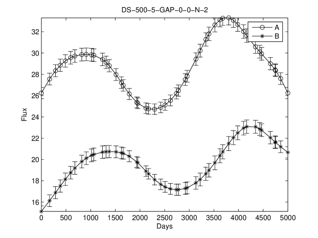
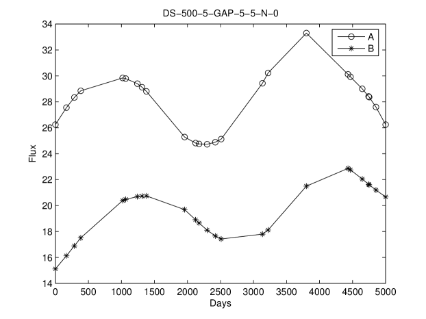
The basic signal is constructed by superimposing $G=20$ Gaussian functions with centres and widths generated randomly. The width is allowed to vary from zero up to a quarter of the duration of the entire monitoring campaign. Then, two artificial fluxes are created by scaling and shifting the basic signal in the flux density and time domains, respectively. The amplitude and flux densities are similar to radio data, 4 cm (Haarsma et al. 1999). The flux ratio was set to $M=1/1.44$ and the temporal shift was equal to $\Delta=500$ days. The time goes from 0 to $T\cdot\Delta$ days with $s_{1}$ samples per $\Delta$ days ($T=10$ and $s_{1}=5$), i.e. if the samples were regularly sampled, we would have a separation of $z=\Delta/s_{1}$ days between samples. To irregularly sample, we disturb the regular observation times with a random variable uniformly distributed in $[-P\cdot z,+P\cdot z]$, $P=0.49$. Moreover, we simulated continuous gaps in observations by imposing $g=5$ blocks of missing data. The blocks are located randomly with at least one sample between them. We worked with block lengths $s_{2}=1,2,...,5$ (see Table 2).

Three levels of noise were used to contaminate the flux signal: 1%, 2% and 3% of the flux; these represent our measurement errors $\sigma_{A}(t_{i})$ and $\sigma_{B}(t_{i})$, which are standard deviations of the flux distribution at each observation time (see Eqs. (1) and (2)). Fig. 2 shows an example of a couple of scaled and shifted artificial fluxes.

Figure 2: Artificial flux data generated to simulate a couple of scaled and shifted fluxes coming from a quasar through a gravitational lens. The top plot shows the underlying function without observational gaps. Also shown are the error bars of 2% of the flux value. Below are the same noise-free fluxes with imposed observational gaps of length 5.

We used $20$ different underlying functions (basic signals). For each underlying function, we generated $100$ realisations for each noise level by adding a Gaussian noise to the underlying function as in equations (1) and (2). For each such data set, we performed $10$ realisations of missing observational blocks. Overall, we employed $307\,020$ different data sets, $15\,351$ data sets per underlying function (see Table 2).

Table 2: Artificial data sets under analysis

	Gap size $s_{2}$
Noise	0	1	2	3	4	5
0%	1	10	10	10	10	10
1%	100	1 000	1 000	1 000	1 000	1 000
2%	100	1 000	1 000	1 000	1 000	1 000
3%	100	1 000	1 000	1 000	1 000	1 000
Sub-Total	301	3 010	3 010	3 010	3 010	3 010
Total = 15 351 data sets per underlying function.
20 underlying functions yield 307 020 data sets.

5 Experiments with artificial data

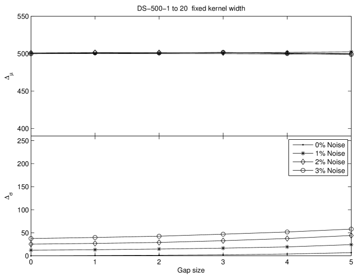
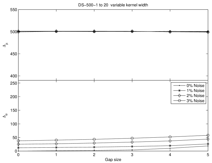
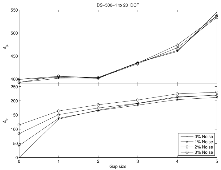
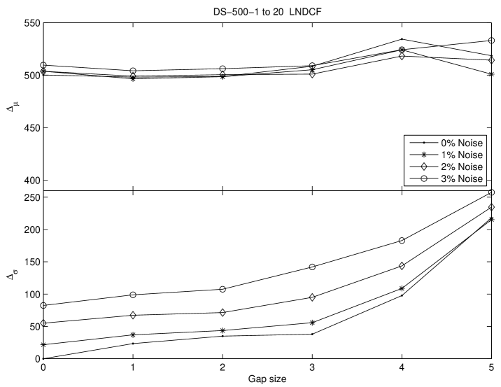
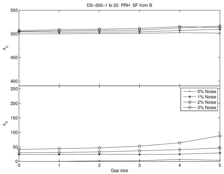
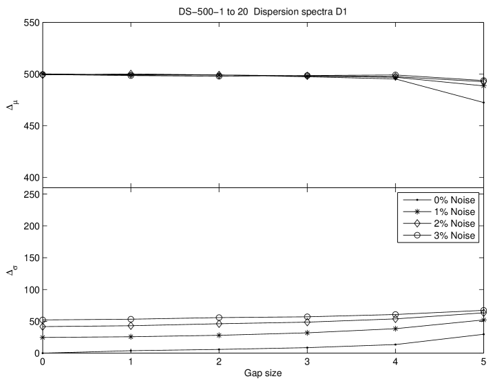
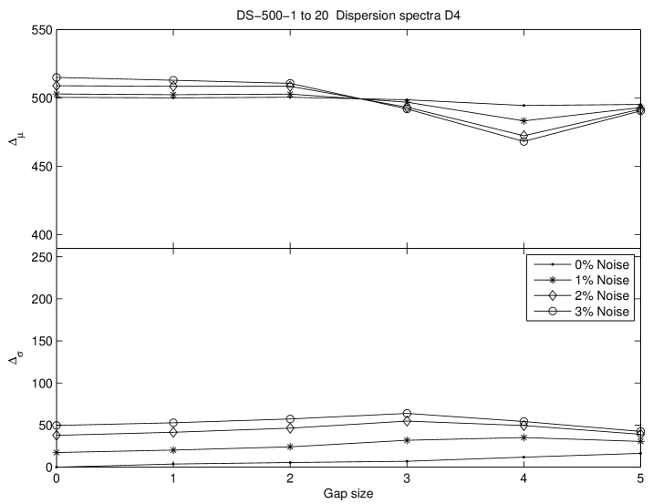
In this section, we test our methods of §2.2.1 and §2.2.2 on artificial data sets described in §4 and compare them to the existing methods described in §3.1, §3.2 and §3.3. Figures 3–10 show two kinds of curves. The top panel shows curves representing the mean estimated time delay $\Delta_{\mu}$ versus the gap size for different noise levels, while lower curves represent means of standard deviations $\Delta_{\sigma}$ of the estimated time delay per underlying function. The quantities of data sets involved in this analysis are shown in Table 2.

In all experiments reported in this section, the following parameter settings were used: $M=1/1.44$, $\Delta_{min}=400$ and $\Delta_{max}=600$ with increments of $1$ day. We used a threshold of $0.001$ (found empirically) to regularise inversion in Eq. 14 through SVD, discarding singular values less than the threshold (Press et al. 1986, §2).

Results for the fixed kernel width technique (Algorithm 1) are shown in Fig. 3. Here, ${\it LowerBound}\!=\!900$ and ${\it UpperBound}\!=\!1200$ with increments of $10$. Fig. 4 shows results of the variable kernel width technique. We fixed the number of neighbours to $k=3$, which was estimated through cross-validation (see Algorithm 1) with ${\it LowerBound}\!=\!1$ and ${\it UpperBound}\!=\!15$ with increments of $1$.

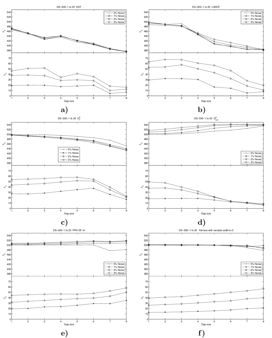
Figures 5 and 6 contain results for the DCF and LNDCF methods respectively. For both methods, bin size of $100$ days (which is close to the lag average) was used and a search was performed for the maximum correlation on bins in the range of $0$ to $2\Delta$ days ($\Delta=500$ for artificial data). We tested DCF and LNDCF on regularly sampled data sets as in §4 (each bin contains those pairs with the same lag). We found that LNDCF never fails, but DCF fails for some shapes of the underlying function (e.g. flat shapes). So, we recommend the use of LNDCF, in preference to DCF.

Figure 7 displays the results of the PRH method using image A to estimate the structure function (23), while Fig. 8 shows results obtained using structure function estimated on image B. When estimating the structure function for each data set in Table 2, we use bins in the range $100-700$ days (Haarsma et al. 1999). Linear regression was used to estimate parameters $c_{1}$ and $c_{2}$ in (24). As pointed out in §3.2, some artificial data sets yield a negative slope due to gaps, high noise and flat features on some underlying functions (when $s_{2}\geq 3$ and noise $\geq 2$%). Therefore, in such cases, we omit them to get more reliable results. Also, we regularise as above to invert $\@vec{B}$ (19), because zero noise and duplicate times may occur in $\@vec{y}$ (18) leading to singularity. Consequently, we do not use the fast methods to get $\@vec{A}$ in (19) (see Rybicki & Press 1995).

The results of the Dispersion spectra method are in Figs. 9 and 10 for $D_{1}^{2}$ and $D_{4,2}^{2}$ respectively. We set $\delta=100$ as decorrelation length for $D_{4,2}^{2}$.

We point out that the results in Figs. 3 to 10 were obtained on the same collection of artificial data sets and are plotted with the same scale on the y-axis. Compared to the existing methods (DCF, LNDCF, PRH, Dispersion spectra), our methods are more accurate and robust with respect to the increasing gap size and noise level. In general, for all methods, there is an obvious tendency of increased uncertainty as the gap size increases. Increasing noise levels in the data result in increased uncertainty of the time delay estimates.

We also tested our method on (annual) periodic gaps ranging from 1 to 8 months, corresponding to observing seasons from 4 to 11 months. The results are in Fig. 11 f). The performance of DCF, LNDCF, Dispersion spectra and PRH method (structure function from image A only) on periodic gaps is also depicted in Fig. 11. The parameters of methods were estimated as above, except for DCF and LNDCF where now we look for a maximum correlation between 400 and 600 days (showing less variance $\Delta_{\sigma}$); sometimes the time delay is below 400 days because we adopt a lower bin if there is no bin of 400 days. We see again that our method outperforms others.

Figure 3: Results of the application of our Kernel method with fixed width (in §2.2.1) on all artificial data sets (see §4). Details in §5.

Figure 4: Results of the application of our Kernel method with variable width (in §2.2.2) on all artificial data sets (see §4). Details are in §5.

Figure 5: Results of the application of the DCF method (in §3.1) on all artificial data sets (see §4). Details are in §5.

Figure 6: Results of the application of the LNDCF method (in §3.1) on all artificial data sets (see §4). Details are in §5.

Figure 7: Results of PRH method with structure function from image A (in §3.2) on all artificial data sets (see §4) except those cases where negative slope occur (355 cases). Details in §5.

Figure 8: Results of the application of the PRH method with structure function from image B (in §3.2) on all artificial data sets (see §4) except those cases where negative slope occur (105 cases). Details are in §5.

Figure 9: Results of the application of the Dispersion spectra method $D_{1}^{2}$ (in §3.3) on all artificial data sets (see §4). Details are in §5.

Figure 10: Results of the application of the Dispersion spectra method $D_{4}^{2}$ (in §3.3) on all artificial data sets (see §4). Details are in §5.

Figure 11: Results on artificial data sets with periodic gaps, see §4 and §5. All plots have the same y-axis scale, and the results are on the same data sets but with different method: a) DCF with bin size $\Delta\tau=100$ (see §3.1), b) LNDCF with bin size $\Delta\tau=100$ (see §3.1), c) Dispersion spectra $D_{1}^{2}$ (see §3.3). d) Dispersion spectra $D_{4,2}^{2}$ with $\delta=100$ (see §3.3), e) PRH method with structure function from image A (see §3.2), and f) Kernels with variable width $k=3$ (see §2.2.2). The results are similar to those in Figs. 4 to 10, respectively. See §5 for more details.

6 Artificial data sets through PRH method

A possible criticism of our testing framework in §4 may be that we construct artificial underlying functions (fluxes) as linear superpositions of Gaussian functions, while our proposed model is a linear superposition of Gaussian kernels (see (1)–(5)). However, widths of the Gaussian functions used to construct the underlying functions are much larger than widths of Gaussian kernels in our model formulation, and so this criticism is less relevant. Still, in order to properly address this issue, we let the PRH method ”play at its own game” by constructing a set of underlying functions using PRH method with a specified structure function (SF). We refer to such data sets as artificial PRH data. These are Monte Carlo time series, generated exactly as described in Press et al. (1992, §5.2), with a fixed SF given by $c_{1}=1/5.36\times 10^{5}$ and $c_{2}=0.246$ (Vanden Berk et al. 2004; Pindor 2005). We use a monitoring campaign length of 8 months with different sampling rates: (i) Low, every seven days. (ii) High, every three days. (iii) Irregular, every two days with periodic gaps of fifteen days (Eigenbrod et al. 2005). (iv) Irregular, as in §4 with lags of 3 days.

We randomly choose seven time delays in the range of 30–100 days. For each combination of time delay and sampling rate, we generate 100 Monte Carlo data sets. To simulate observational errors, we use fixed variances of $1\times 10^{-7}$ and $1\times 10^{-9}$ in order to get distinguishable shapes by eye, i.e. low noise. Then, we analyse all the artificial PRH data sets with our methods in §2 and the PRH method as described in §3.2.

If we keep the SF (i.e. $c_{1}$ and $c_{2}$) fixed to its true value (as assigned to the simulations), then the performance of the PRH method is outstanding, with almost zero bias and zero variance for all data sets as a whole. However, the performance is not always as good when applied to individual data sets (one realisation). Further, if we assume that we do not know the true SF used to generate the data, and we estimate it through the data itself (see §3.2), then our methods perform better than the PRH method, as shown in the case of the artificial data in §4 (see Table 3). In fact, one is unable to recover the true SF from the Monte Carlo data sets. Table 3 shows results for the third case of sampling only, since others give similar results.

Table 3: Results on PRH data: irregular sampling and periodic gaps only, observational errors with variance $1\times 10^{-7}$, see §6.

$\Delta$	PRH*	PRH**	Kernels***
True delay	mean$\pm$std	mean$\pm$std	mean$\pm$std
34	34.0$\pm$2.3	23.2$\pm$21.9	33.9$\pm$10.3
43	43.1$\pm$4.7	45.0$\pm$16.2	43.4$\pm$2.4
49	50.6$\pm$7.0	47.2$\pm$17.5	48.8$\pm$6.9
59	60.0$\pm$5.5	58.9$\pm$21.4	59.8$\pm$10.4
66	66.0$\pm$2.5	63.3$\pm$23.2	66.6$\pm$9.1
76	76.7$\pm$3.8	71.1$\pm$22.2	75.5$\pm$11.5
99	100.9$\pm$7.2	97.2$\pm$21.1	103.2$\pm$12.5
*     PRH method with SF fixed to true values $c_{1}$ and $c_{2}$.
**   PRH method with SF estimated from the data, image A.
*** Kernels with variable width $k=3$.

7 The gravitational lens Q0957+561: radio observations

In this section we apply the tools developed in this paper to estimate the time delay for the much studied quasar Q0957+561. We use radio monitoring data at 4 cm and 6 cm wavelengths. For the 6 cm data set, we use the light curve with four points from Spring 1990 removed, as in (see Haarsma et al. 1999), . These radio data sets are plotted at the top in Fig. 1. Our results are presented in Table 4.

To estimate the time delay for this quasar, we use both the fixed kernel width and variable kernel width approaches outlined in §2. We employ flux ratios $M=1/1.44$ and $M=1/1.43$ for the 4 cm and 6 cm data, respectively (the most likely values given our models). We tested time delays between $\Delta_{min}=300$ and $\Delta_{max}=500$, with increments of $1$ day. As in the previous section, we use a threshold of $0.001$ when regularising matrix inversion through SVD. The noise model is assumed to be zero mean i.i.d. Gaussian with standard deviation of $2$% of the observed flux value.

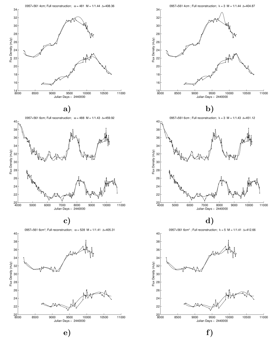
For the fixed kernel width technique (§2.2.1), we use Algorithm 1 with the following parameters: $LowerBound=100$ and $UpperBound=1200$ with increments of $1$ day, The selected kernel widths ($\omega$) were $481$ and $488$ days, and the estimated time delays were 409 days and 459 days for the 4 cm and 6 cm bands, respectively. To calculate confidence intervals on our time delay estimates, we performed 500 Monte Carlo simulations by adding noise realisations to the observed data. Confidence intervals were determined as standard deviations of time delay estimates across the Monte Carlo samples. We found delays of 408$\pm$10 days and 460$\pm$18 days for 4 cm and 6 cm respectively. Flux reconstructions with these time delays are shown in in Figs. 12 a) and 12 b).

For the variable kernel width method (§2.2.2), the number of neighbours $k$ determining local kernel widths was estimated by Algorithm 1 ($\omega$ is replaced by $k$) with $LowerBound=1$ and $UpperBound=15$ (increments of $1$). We obtained $k=3$ for 4 cm, and the estimated time delay was 405 days. Confidence interval computed on 500 Monte Carlo samples was 404.8$\pm$11. Flux reconstructions with this time delay are shown in Fig. 12 c). For 6 cm data, we found $k=3$, and the delay of 450 days. The 500 Monte Carlo samples gave us a time delay of 451.1$\pm$30 days. Flux reconstructions are presented in Fig. 12 d).

Using the PRH method, Haarsma et al. (1999) report time delays of 397$\pm$12 and 452${}_{-15}^{+14}$ days for the 4 cm and 6 cm data, respectively, and 409$\pm$30 on the combined 4+6 cm data set. They also report results of the Dispersion spectra method: 383${}_{-19}^{+15}$ and 416${}_{-24}^{+22}$ days for the 4 cm and 6 cm data, respectively, and 395${}_{-15}^{+13}$ days on the combined 4+6 cm data set.

There has been a great deal of concern about the difference in time delay estimates from the two different wavelengths, since gravitational lensing is achromatic. Inspired by the results from our experimentation with artificial data, where the uncertainty of time delay estimates increases as the gap size increases, we have generated a new data set, 6 cm*, in order to avoid the effect of the different gap sizes for different wavelengths. The 6 cm* data set contains 6 cm observations sampled only at observation times of the 4 cm dataset. In other words, we keep a 6 cm observation at time $t$ if there is a 4 cm observation at the same time $t$. The 4 cm and 6 cm* data sets both contain 58 observations.

Time delay estimates obtained by our methods on 500 Monte Carlo samples based on the 6 cm* data set are presented in Table 4. The ‘optimal’ kernel parameters, $\omega=528$ and $k=5$, are obtained following the procedure described above. The estimated time delays are 405 days and 412 days for the fixed kernel width and variable kernel width methods, respectively. The resulting flux reconstructions are shown in Figs. 12 e) and 12 f).

On comparing the 4 cm and 6 cm* samples, which are pairs of the observations at the same epoch and thus have identical gaps in the time series, we find a consistent value for the estimated time delay. This exercise indicates that the disagreement between the 4 cm and 6 cm datasets is largely due to sampling and systematic errors.

Table 4: The time delay between Q0957+561 A & B estimated from radio “light” curves at 4 cm and 6 cm.

Kernel method:	fixed width	variable width
4 cm	408.3$\pm$10	404.8$\pm$11
6 cm	459.9$\pm$18	451.1$\pm$30
6 cm*	405.3$\pm$29	412.6$\pm$35
Note: The time delays are in days.
The construction of the 6 cm* sample, which contains
only the 6 cm observations that have a corresponding 4 cm
observation at the same epoch, is described in §7.

Figure 12: Radio observations of gravitationally lensed images A & B of Q0957+561. We show reconstructions with fixed parameters: a) 4 cm with fixed width ($\omega=481$, $\Delta=408.3$), b) 4 cm with variable width ($k=3$, $\Delta=404.8$), c) 6 cm with fixed width ($\omega=488$, $\Delta=459.9$), d) 6 cm with variable width ($k=3$, $\Delta=451.1$), e) 6 cm* with fixed width ($\omega=528$, $\Delta=405.3$), and f) 6 cm* with variable width ($k=5$, $\Delta=412.6$). Within each plot, at the top is the image A and at the bottom is image B. The continuous lines are our reconstructed underlying light curves, $h_{A}(t_{u})$ and $h_{B}(t_{v})$ in Eq. 9.

It is evident that the large variation in the estimates in the values of time delay, measured in several analyses of the same observed data sets that we analyse in this paper, is due to the presence of the gaps in the monitoring at the two wavelengths. Such gaps are unavoidable in realistic long-term observing programmes, often leading to unacceptably deviant time delays (in this case, too large by more than 10%). Several recent analyses have come to this conclusion in various ways (e.g. Gil-Merino et al. 2002; Pindor 2005; Eigenbrod et al. 2005).

Table 5: Results from experiments with artificial data sets.

Method	Figure
Kernel method with fixed width	Fig. 3
Kernel method with variable width	Fig. 4
DCF and LNDCF	Figs. 5 and 6
PRH method, Structure function from A	Fig. 7
PRH method, Structure function from B	Fig. 8
Dispersion spectra ($D_{1}^{2}$ and $D_{4,2}^{2}$)	Figs. 9 and 10

8 Conclusions

We have introduced a new way of measuring the time delay between light curves of two images of a gravitationally lensed system, based on generalised linear regression with fixed- and variable-width Gaussian basis functions (Kernels) (see §2.2.1 and §2.2.2). On a large set of controlled experiments using artificially generated data, we compare the accuracy of our methods with that of other methods used in the literature for time delay estimation, notably the DCF, LNDCF, PRH and Dispersion spectra methods (see Table 5).

Running a controlled set of experiments is essential for a well-grounded comparison of competing models. For the artificial data, unlike in the case of observed fluxes, we have the luxury of knowing exactly the magnification ratio $M$ and the time delay $\Delta$; the noise process is also known. Therefore, we can reliably measure the bias ($\Delta_{\mu}$, top of Figs. 3–10) and variance ($\Delta_{\sigma}$, bottom of Figs. 3–10) of the time delay estimates given by the studied methods. Obviously, one can never fully measure the bias when estimating the time delay from real observations. On the artificial data, our kernel-based methods presented in this paper came across as the most accurate and stable methodologies for estimating the time delays between multiple images of a gravitationally lensed quasar.

Previous attempts at generating similar artificial data have tried to simulate specific data sets (see Pijpers 1997; Burud et al. 2001). Our artificial data sets contain simulated light curves of widely varying (but still realistic) shapes, observational gaps and noise levels (these can be made available on request – see more plots at http://www.cs.bham.ac.uk/$\sim$jcc/artificial). At the bottom of Figs. 3–10, we can observe a general trend of increased uncertainty as the gap size increases. The uncertainty is also proportional to the noise level.

Our methods for estimating the time delay introduced in sections §2.2.1 and §2.2.2, give similar results (see Figs. 3 & 4), although the variable kernel width method tends to require less computational time.

Finally, we have estimated the time delay between of two images of the quasar Q0957+561 from radio observations at 4 cm and 6 cm. The time delay estimates given by our methods are in the range of 405–412 days (see Table 4), which are lower than, but consistent with, most of the other estimates from the same or similar radio data sets (see §7). However, the 6 cm* data set, which by construction includes only observations that are performed at the same epoch as those in the 4 cm data set, yields essentially the same value for the time delay at that obtained from the 4 cm data set (these can be combined to yield $408\pm 12$ days, the errors being lower for just the 4 cm data), as opposed to a value of $\sim$450 days as obtained from the full 6 cm data set, which covers a longer monitoring period.

We conclude that such systematic differences between results obtained from observations at various wavelengths are due to the irregular sampling, and in particular, due to the presence of large gaps in the monitoring data. Experiments with simulated data sets like ours help in the understanding of how the results depends on the sampling, and in assessing the reliability of the time delays obtained by various methods.