Wronskian Formulation of the Spectrum of Curvature Perturbations

Abstract

We present a new formulation for the evaluation of the primordial spectrum of curvature perturbations generated during inflation, using the fact that the Wronskian of the scalar field perturbation equation is constant. In the literature, there are many works on the same issue focusing on a few specific aspects or effects. Here we deal with the general multi-component scalar field, and show that our new formalism gives a method to evaluate the final amplitude of the curvature perturbation systematically and economically. The advantage of the new method is that one only has to solve a single mode of the scalar field perturbation equation backward in time from the end of inflation to the stage at which the perturbation is within the Hubble horizon, at which the initial values of the scalar field perturbations are given. We also clarify the relation of the new method with the new $\delta N$ formalism recently developed in Ref. ref4 .

I Introduction

Inflation provides an elegant mechanism to solve shortcomings of the standard Big Bang Model, for example, the flatness and horizon problems. Moreover, in the inflationary universe, curvature perturbations, which seed the structure formation of the universe, are generated from vacuum fluctuations of the scalar field. One can test various models of inflation, by comparing the theoretical prediction for the spectrum of curvature perturbations with observations.

In single-field slow-roll inflation models, curvature perturbations evaluated on comoving hypersurfaces, ${\cal R}_{\rm c}$, are constant on super-horizon scales, and their spectrum is given by

$${\cal P}_{{\cal R}_{\rm c}}(k)\sim\left(\frac{H^{2}}{2\pi\dot{\phi}}\right)^{2}_{aH=k},$$ (1)

where $H$ is the Hubble parameter, $\dot{\phi}$ is the derivative of the inflaton $\phi$ with respect to the cosmological time, and the subscript “$aH=k$” means that the expression is to be evaluated at the horizon crossing time, $t=t_{k}$. This equation indicates that the spectrum of the primordial curvature perturbations is almost scale-invariant in slow-roll inflation models composed of a single scalar field.

However, in making realistic models of inflation based on supersymmetry and supergravity theories, it seems more natural to consider models composed of a multi-component scalar field, in which the slow-roll conditions are also possibly violated Kadota:2003fs . Obviously, Eq. (1) is not sufficient to evaluate the spectrum of the curvature perturbations generated in such models. In order to identify necessary conditions for viable models of inflation among various proposed possibilities, any simple and sufficiently accurate formula for the spectrum is useful, especially if the formula is applicable to a wide class of models.

There are several works aiming at generalizing the slow-roll formula (1) in the case of a single scalar field. For example, Leach, Sasaki, Wands and Liddle ref2 have analyzed the evolution of curvature perturbations on superhorizon scales (the long-wavelength approximation). They have found that the curvature perturbations can be enhanced when $z\equiv a\dot{\phi}/H$ decreases after the horizon crossing time $t_{k}$. This situation can happen if the slow-roll conditions are violated for $t>t_{k}$. On the other hand, Stewart ref3 has generalized the standard formula (1), removing the extra assumption that slow-roll parameters are approximately scale invariant, and this generalization is called the general slow-roll approximation. Under the conditions which lead to the standard slow-roll formula (1), the running of spectrum is automatically suppressed as $\left|dn_{\cal R_{\rm c}}/d\ln k\right|\ll\left|n_{\cal R_{\rm c}}-1\right|$, while under the general slow-roll conditions, $\left|dn_{\cal R_{\rm c}}/d\ln k\right|$ can be as large as $|n_{\cal R_{\rm c}}-1|$. These conditions are consistent with recent observational data WMAP ; Spergel:2006hy .

For multi-component inflation, evaluating the curvature perturbations is a more difficult issue in comparison with single-component inflation SS ; ST ; multi ; Wands:2000dp ; Nakamura:1996da ; Salopek:1988qh ; Bartolo:2001rt ; Hwang:1999gf ; Starobinsky:1994mh ; Polarski:1994rz ; Garcia-Bellido:1996ke ; Langlois:1999dw ; Kadota:2003fs . Generally, in the case of a $D$-component field, the evolution equations for the perturbations are $D$ coupled second order differential equations. It is a heavy task to solve the full set of equations. Moreover, for multi-component inflation, the curvature perturbations on comoving slices, $\mathcal{R}_{c}$, still varies in time on super-horizon scales until the neighboring trajectories of the background homogeneous universe in the phase space practically converge to a single one. It is after the convergence of the trajectories that $\mathcal{R}_{c}$ becomes constant in time SS ; ST .

However, in the estimation of the spectrum, what we need is only the final value of the curvature perturbation $\mathcal{R}_{c}(\eta_{f})$. Here, $\eta$ is a conformal time given by $\eta=\int dt/a$, and $\eta_{\rm\,f}$ is taken sufficiently late after the convergence of the background trajectories. So, if we can identify the part of perturbations that contributes to $\mathcal{R}_{c}(\eta_{f})$, we may solve only that part to obtain its value without solving the full set of perturbation equations. The $\delta N$ formalism SS ; ST was based on this idea, and we have developed a new $\delta N$ formalism ref4 . This formulation was developed based on the fact that the perturbation of $e-$folding number stays roughly constant in the flat slicing on super-horizon scales. We derived a perturbation equation for a single projected component of scalar field corresponding to the perturbation of $e-$folding number. The derivation of the new $\delta N$ formalism is rather intuitive in this sense, which helps to make its physical meaning rather transparent. As a drawback, however, the systematical derivation of the formula is not so simple. Moreover, in Ref. ref4 we only applied our new formalism to cases without the possible super-horizon contributions pointed out in Ref. ref2 , postponing this generalized application to Ref. future . Here we propose an alternative slightly different framework to evaluate the evolution of perturbations of a multi-component scalar field. The method we will discuss in this paper takes full advantage of the fact that the Wronskian stays constant.

This paper is organized as follows. In section II, we briefly explain the perturbation equations for multi-component scalar field in the flat slicing. In section III, we introduce a Wronskian between two solutions of perturbation equations, and explain how we can use it in evaluating the curvature perturbation at a later time $\eta=\eta_{f}$. As far as we are concerned with the evolution during the phase dominated by the scalar field, what we have to do turns out to be just solving a single mode backward in time with appropriate boundary conditions imposed at $\eta=\eta_{\rm\,f}$. In section IV, we use the Wronskian to derive more explicit analytic expressions for the spectrum of perturbations. We consider an extension of the general slow-roll formula developed in Ref. ref3 ; ref4 , combining it with the long wavelength approximation ref2 , which suites for describing the late time evolution future . We assume that the general slow-roll approximation is valid until a time $\eta_{*}$ later than the horizon crossing time $\eta_{k}$, and we use the long-wavelength approximation for the succeeding evolution until the end of inflation, $\eta_{f}$. To combine the two solutions obtained by using different approximation schemes in the matching region where both approximations are valid, we find that the constancy of the Wronskian is again very useful. The derived new analytic formula applies for a wider class of multi-component inflation models. In section V, we reduce the obtained formula to the single-field case. In this case, the formula for the spectrum can be expressed more explicitly. Using our new formulation, it is also easy to see that the amplitude of perturbation stays regular even if the time derivative of $\phi$ vanishes, as was discussed in Ref. Seto . In section VI, we present a brief summary.

II Perturbation equations for multi-component scalar field

We consider a $D$-component scalar field whose action is given by

$$S_{{\rm matter}}=-\int d^{4}x\sqrt{-g}\left[\frac{1}{2}g^{\mu\nu}\delta_{\alpha\beta}\partial_{\mu}\phi^{\alpha}\partial_{\nu}\phi^{\beta}+V(\phi)\right]~{},$$ (2)

where, for simplicity, we have chosen to work with the flat metric $\delta_{\alpha\beta}$ for the scalar field space, because the equations will be more involved for the general field space metric and hence the essence of our new formulation may be obscured, though the extension to the general metric case is straightforward. The background equations are

$$3{\cal H}^{2}=\frac{1}{2}\delta_{\alpha\beta}{\phi^{\alpha}}^{\prime}{\phi^{\beta}}^{\prime}+a^{2}V(\phi)~{},$$ (3)

$${\phi^{\alpha}}^{\prime\prime}+2{\cal H}{\phi^{\alpha}}^{\prime}+a^{2}\delta^{\alpha\beta}V_{,\phi^{\beta}}=0~{},$$ (4)

where ${\cal H}\equiv a^{\prime}/a$, the prime represents a derivative with respect to the conformal time $\eta$, and $V_{,\phi^{\alpha}}\equiv\partial V/\partial\phi^{\alpha}$.

We consider only scalar type perturbations. Then the perturbed metric is given by KS

$$ds^{2}=a^{2}\left\{-(1+2AY)d\eta^{2}-2BY_{j}d\eta dx^{j}+\left[(1+2H_{L}Y)\delta_{ij}+2H_{T}Y_{ij}\right]dx^{i}dx^{j}\right\}~{},$$ (5)

where $Y$ is the spatial scalar harmonic function with the eigenvalue $k^{2}$, $Y_{j}\equiv-k^{-1}\nabla_{j}Y$, and $Y_{ij}\equiv\left(k^{-2}\nabla_{i}\nabla_{j}+\frac{1}{3}\delta_{ij}\right)Y$.

We decompose the scalar field to the background and perturbations as

$$\tilde{\phi}=\phi(\eta)+\delta\phi(x^{\mu})Y~{},$$ (6)

and define a gauge invariant variable

$$\delta\phi_{F}^{\alpha}\equiv\delta\phi^{\alpha}-\frac{{\phi^{\alpha}}^{\prime}}{{\cal H}}{\cal R}~{},$$ (7)

which represents the scalar field perturbation on the flat slicing. Here

$${\cal R}\equiv H_{L}+\frac{1}{3}H_{T}~{},$$ (8)

represents the intrinsic curvature perturbation of the constant time hypersurfaces. The evolution equation for $\delta\phi^{\alpha}_{F}$ is known to be given by SS

$$\left\{\partial_{\eta}^{2}-\left({\cal H}^{2}+{\cal H}^{\prime}\right)+k^{2}\right\}\varphi^{\alpha}=\left\{\frac{1}{a^{2}}\left(\frac{a^{2}{\phi^{\alpha}}^{\prime}{\phi^{\gamma}}^{\prime}}{{\cal H}}\right)^{\prime}\delta_{\gamma\beta}-a^{2}\delta^{\alpha\gamma}V_{,\phi^{\gamma}\phi^{\beta}}\right\}\varphi^{\beta}~{},$$ (9)

where

$$\varphi^{\alpha}\equiv a\delta\phi^{\alpha}_{F}.$$ (10)

III Use of Wronskian

When we calculate the curvature perturbation spectrum, we only need the final value of the curvature perturbation, $\mathcal{R}_{c}(\eta_{f})$. We do not need to know the evolution of all components of the multi-component field. In other words, if we can identify the part of the perturbations that contributes to $\mathcal{R}_{c}(\eta_{f})$, we may be able to solve only the necessary part without obtaining a full set of solutions of perturbation equations.

The equation (9) is an equation which formally takes the form of

$$\left[\partial_{\eta}^{2}+Q(\eta)+k^{2}\right]\varphi^{\alpha}=P^{\alpha}_{~{}\beta}(\eta)\varphi^{\beta},$$ (11)

with $P^{\alpha}_{~{}\beta}$ symmetric with respect to the indices $\alpha$ and $\beta$. The Wronskian

$$W({{\mbox{\boldmath$n$}}{\mbox{\boldmath$n$}}{\mbox{\boldmath$n$}}},{{\bm{\varphi}}{\bm{\varphi}}})\equiv{{\mbox{\boldmath$n$}}{\mbox{\boldmath$n$}}{\mbox{\boldmath$n$}}}^{\prime}\cdot{{\bm{\varphi}}{\bm{\varphi}}}-{{\mbox{\boldmath$n$}}{\mbox{\boldmath$n$}}{\mbox{\boldmath$n$}}}\cdot{{\bm{\varphi}}{\bm{\varphi}}}^{\prime},$$ (12)

introduced in a usual manner is constant if $n$$n$$n$ and ${{\bm{\varphi}}{\bm{\varphi}}}$ are solutions of Eq. (11). Here we used vector notation $n$$n$$n$ and ${{\bm{\varphi}}{\bm{\varphi}}}$ to represent $n^{\alpha}$ and $\varphi^{\alpha}$ for brevity and ${{\mbox{\boldmath$n$}}{\mbox{\boldmath$n$}}{\mbox{\boldmath$n$}}}\cdot{{\bm{\varphi}}{\bm{\varphi}}}\equiv\delta_{\alpha\beta}n^{\alpha}\varphi^{\beta}$.

As is known well, when the universe is dominated by a single matter component whose physical state is solely characterized by a single parameter, say, the energy density as in the case of a slowly rolling scalar field or a single component perfect fluid, the curvature perturbation on comoving hypersurfaces ${\cal R}_{c}$ is constant in time on super-horizon scales. If the background trajectories in the phase space of the multi-component scalar field well converge to a single one at a time, $\eta_{\rm con}$, before the scalar field dominant phase ends, the system is effectively equivalent to a single scalar field for $\eta>\eta_{\rm con}$. In such cases the problem is relatively easy to formulate. In comoving gauge, $\delta_{\alpha\beta}{\phi^{\alpha}}^{\prime}\delta\phi^{\beta}=0$ by definition. Contracting Eq. (7) with ${\phi}_{\alpha}^{\prime}=\delta_{\alpha\beta}{\phi^{\beta}}^{\prime}$, we find

$${\cal R}_{c}=-{{\cal H}{{\mbox{\boldmath$\phi$}}{\mbox{\boldmath$\phi$}}{\mbox{\boldmath$\phi$}}}^{\prime}\cdot{{\bm{\varphi}}{\bm{\varphi}}}\over a{{{\mbox{\boldmath$\phi$}}{\mbox{\boldmath$\phi$}}{\mbox{\boldmath$\phi$}}}^{\prime}}^{2}}.$$ (13)

Hence, by defining $n$$n$$n$ so that it satisfies the boundary conditions

$${{\mbox{\boldmath$n$}}{\mbox{\boldmath$n$}}{\mbox{\boldmath$n$}}}^{\prime}=-{{\cal H}{{\mbox{\boldmath$\phi$}}{\mbox{\boldmath$\phi$}}{\mbox{\boldmath$\phi$}}}^{\prime}\over a{{{\mbox{\boldmath$\phi$}}{\mbox{\boldmath$\phi$}}{\mbox{\boldmath$\phi$}}}^{\prime}}^{2}},\qquad{{\mbox{\boldmath$n$}}{\mbox{\boldmath$n$}}{\mbox{\boldmath$n$}}}=0,$$ (14)

at $\eta=\eta_{\rm con}$, the above Wronskian agrees with ${\cal R}_{c}$:

$${\cal R}_{c}(\eta_{\rm con})=W({{\mbox{\boldmath$n$}}{\mbox{\boldmath$n$}}{\mbox{\boldmath$n$}}},{{\bm{\varphi}}{\bm{\varphi}}}).$$ (15)

Since the Wronskian is constant, it can be evaluated at any time. Therefore, once $n$$n$$n$ is solved backward in time until the wavelength of the mode is well inside the horizon scale with the appropriate boundary conditions, Eq. (14), we do not have to evolve ${{\bm{\varphi}}{\bm{\varphi}}}$ at all in the forward direction. This will be advantageous in the case of a multi-component field. In order to solve ${{\bm{\varphi}}{\bm{\varphi}}}$ in the forward direction, we need to solve all $2D$ independent modes, where $D$ is the number of species. In contrast, to evolve $n$$n$$n$ backward in time, we only need to solve a single mode. Hence, the advantage of solving $n$$n$$n$ instead of ${{\bm{\varphi}}{\bm{\varphi}}}$ becomes prominent as the number of species increases. An extreme example is the models with extra-dimensions RubakovKobayashi . Since $D$ is infinite in the brane world models, solving for all ${{\bm{\varphi}}{\bm{\varphi}}}$ is impossible. Note that the boundary condition (14) is given solely in terms of the background quantities. This implies that $n$$n$$n$ is uniquely determined for arbitrary scalar field perturbations.

In general multi-component models, it may not be a good assumption to assume that the trajectories converge to a single one before the scalar dominant phase terminates. Once the convergence of trajectories occurs, the universe undergoes a universal evolution everywhere, and the only remaining modes of scalar-type perturbations are adiabatic ones SS . If we do not consider the case with isocurvature perturbations that persist until the present epoch, we can assume that the convergence of trajectories occurs at a certain time, but it need not happen during the scalar dominant phase. In multi-component models, the convergence of trajectories may occur in general after complete reheating SS ; ref4 . In such cases it is at this stage that $\mathcal{R}_{c}$ becomes constant in time on super-horizon scales.

Even when the trajectories in phase space have not converged, the $\delta N$ formalism SS simplifies the evaluation of the evolution of perturbations in the long wavelength limit. In the rest of this section the long wavelength limit also contains the meaning that we neglect the shear of the constant time hypersurfaces, which rapidly decays on super-horizon scales ST . Let us take $\eta_{\rm\,i}$ to be a certain time soon after the relevant scale have become greater than the horizon scale and $\eta_{\rm\,f}$ to be a certain time after the complete convergence of trajectories. The $\delta N$ formalism is based on the fact that the final value of the curvature perturbation $\mathcal{R}_{c}(\eta_{\rm\,f})$ is given by $\delta{\cal N}(\eta_{\rm\,f},\eta_{\rm\,i})$, the perturbation in the $e$-folding number between the initial flat hypersurface at $\eta=\eta_{\rm\,i}$ and the final comoving hypersurface at $\eta=\eta_{\rm\,f}$ in the long wavelength limit.

The evolution of $\delta{\cal N}$ in the long wavelength limit is expected to be described by the dynamics of the homogeneous universe in the following sense SS ; ST . We define $N$ by the $e$-folding number necessary to reach the point in the phase space corresponding to $\eta_{\rm\,f}$ by solving the evolution of the homogeneous universe. If we choose $\eta_{\rm\,i}$ to be in the scalar dominant phase, $N$ will be a function of $\phi$$\phi$$\phi$ and ${{\mbox{\boldmath$\phi$}}{\mbox{\boldmath$\phi$}}{\mbox{\boldmath$\phi$}}}^{\prime}$. Then, in the super-horizon scales, the perturbation in $N$ is given by

$$\delta N = \left[{\partial N\over\partial{{\mbox{\boldmath$\phi$}}{\mbox{\boldmath$\phi$}}{\mbox{\boldmath$\phi$}}}}\cdot\delta{{\mbox{\boldmath$\phi$}}{\mbox{\boldmath$\phi$}}{\mbox{\boldmath$\phi$}}}_{F}+{\partial N\over\partial\left(d{{{\mbox{\boldmath$\phi$}}{\mbox{\boldmath$\phi$}}{\mbox{\boldmath$\phi$}}}}/d\tau\right)}\cdot\delta\left({d{{\mbox{\boldmath$\phi$}}{\mbox{\boldmath$\phi$}}{\mbox{\boldmath$\phi$}}}\over d\tau}\right)_{F}\right]_{\eta_{\rm\,i}}$$ (16)

$$= \left\{{\partial N\over\partial{{\mbox{\boldmath$\phi$}}{\mbox{\boldmath$\phi$}}{\mbox{\boldmath$\phi$}}}}\cdot\left({{{\bm{\varphi}}{\bm{\varphi}}}\over a}\right)+{\partial N\over\partial{{{\mbox{\boldmath$\phi$}}{\mbox{\boldmath$\phi$}}{\mbox{\boldmath$\phi$}}}}^{\prime}}\cdot\left[\left({{{\bm{\varphi}}{\bm{\varphi}}}\over a}\right)^{\prime}-{{\mbox{\boldmath$\phi$}}{\mbox{\boldmath$\phi$}}{\mbox{\boldmath$\phi$}}}^{\prime}A_{F}\right]\right\}_{\eta_{\rm\,i}}~{}.$$

Here, the subscript $F$ denotes a quantity evaluated on flat hypersurfaces and the subscript $\eta_{\rm\,i}$ denotes a quantity evaluated at $\eta=\eta_{\rm\,i}$. The perturbed proper time $\tau$ satisfies $d\tau=a(1+A)d\eta$, and the perturbation of the lapse function on flat hypersurfaces $A_{F}$ is given by ref4

$$A_{F}={1\over 2}{{{\mbox{\boldmath$\phi$}}{\mbox{\boldmath$\phi$}}{\mbox{\boldmath$\phi$}}}^{\prime}\cdot{{\bm{\varphi}}{\bm{\varphi}}}\over a{\cal H}}.$$ (17)

Thus we obtain

$$\delta N = -W({{\mbox{\boldmath$n$}}{\mbox{\boldmath$n$}}{\mbox{\boldmath$n$}}}_{B},{{\bm{\varphi}}{\bm{\varphi}}})_{\eta_{\rm\,i}},$$ (18)

with

$${{\mbox{\boldmath$n$}}{\mbox{\boldmath$n$}}{\mbox{\boldmath$n$}}}_{B}^{\prime}=-{1\over a}{\partial N\over\partial{{\mbox{\boldmath$\phi$}}{\mbox{\boldmath$\phi$}}{\mbox{\boldmath$\phi$}}}}+{{\cal H}\over a}{\partial N\over\partial{{\mbox{\boldmath$\phi$}}{\mbox{\boldmath$\phi$}}{\mbox{\boldmath$\phi$}}}^{\prime}}+{1\over 2a{\cal H}}\left({\partial N\over\partial{{\mbox{\boldmath$\phi$}}{\mbox{\boldmath$\phi$}}{\mbox{\boldmath$\phi$}}}^{\prime}}\cdot{{\mbox{\boldmath$\phi$}}{\mbox{\boldmath$\phi$}}{\mbox{\boldmath$\phi$}}}^{\prime}\right){{\mbox{\boldmath$\phi$}}{\mbox{\boldmath$\phi$}}{\mbox{\boldmath$\phi$}}}^{\prime},\qquad{{\mbox{\boldmath$n$}}{\mbox{\boldmath$n$}}{\mbox{\boldmath$n$}}}_{B}={1\over a}{\partial N\over\partial{{\mbox{\boldmath$\phi$}}{\mbox{\boldmath$\phi$}}{\mbox{\boldmath$\phi$}}}^{\prime}}.$$ (19)

Our expectation is that, $\delta N$ is identical to $\delta{\cal N}$ in the long wavelength limit in general. In fact, it was shown in Ref. ST that this is indeed the case if $\eta_{\rm\,f}$ also lies in the scalar dominant phase. We plan to discuss this issue in the more general cases in our future publication future . Here in this paper we simply assume $\delta{\cal N}\approx\delta N$ in the long wavelength limit. Notice that the meaning of this approximate equality is an identity relation which holds for any ${{\bm{\varphi}}{\bm{\varphi}}}$ and ${{\bm{\varphi}}{\bm{\varphi}}}^{\prime}$. Hence, $W({{\mbox{\boldmath$n$}}{\mbox{\boldmath$n$}}{\mbox{\boldmath$n$}}},{{\bm{\varphi}}{\bm{\varphi}}})\approx W({{\mbox{\boldmath$n$}}{\mbox{\boldmath$n$}}{\mbox{\boldmath$n$}}}_{B},{{\bm{\varphi}}{\bm{\varphi}}})$ is also to be understood in the same way. Therefore we conclude ${{\mbox{\boldmath$n$}}{\mbox{\boldmath$n$}}{\mbox{\boldmath$n$}}}_{B}\approx{{\mbox{\boldmath$n$}}{\mbox{\boldmath$n$}}{\mbox{\boldmath$n$}}}$. In fact, it has been shown in our previous paper ref4 that ${{\mbox{\boldmath$n$}}{\mbox{\boldmath$n$}}{\mbox{\boldmath$n$}}}_{B}$ defined above is a solution of Eq. (9) in the long wavelength limit. Thus, in the case that the convergence of trajectories occurs after the scalar dominant phase ends, the boundary conditions for $n$$n$$n$ are given by ${{\mbox{\boldmath$n$}}{\mbox{\boldmath$n$}}{\mbox{\boldmath$n$}}}={{\mbox{\boldmath$n$}}{\mbox{\boldmath$n$}}{\mbox{\boldmath$n$}}}_{B}(\eta_{\rm\,i})$ and ${{\mbox{\boldmath$n$}}{\mbox{\boldmath$n$}}{\mbox{\boldmath$n$}}}^{\prime}={{\mbox{\boldmath$n$}}{\mbox{\boldmath$n$}}{\mbox{\boldmath$n$}}}^{\prime}_{B}(\eta_{\rm\,i})$ instead of Eq. (14).

It would be worth mentioning that $n$$n$$n$ used here is a full decaying mode solution obtained without assuming the long wavelength limit, while in Ref. ref4 we used a super-horizon decaying mode solution, which is a solution for Eq. (9) with $k^{2}\to 0$. They are identical only in the long wavelength limit. Here we make full advantage of the constancy of the Wronskian $W({{\mbox{\boldmath$n$}}{\mbox{\boldmath$n$}}{\mbox{\boldmath$n$}}},{{\bm{\varphi}}{\bm{\varphi}}})$. In contrast, in Ref. ref4 we discussed the evolution of the super-horizon Wronskian, which is defined by $W({{\mbox{\boldmath$n$}}{\mbox{\boldmath$n$}}{\mbox{\boldmath$n$}}},{{\bm{\varphi}}{\bm{\varphi}}})$ with $n$$n$$n$ replaced by the super-horizon decaying mode solution.

IV Extended general slow-roll formula

Even if we use the Wronskian method, we still need to solve $n$$n$$n$ backward for each $k$. However, we can avoid solving $n$$n$$n$ for each value of $k$ in the long wavelength limit. In this limit, we can find the solution for $n$$n$$n$ in the series expansion with respect to $k^{2}$. Of course, this approximation does not hold when the wavelength becomes shorter than the horizon scale. For the evolution before the horizon crossing, one may use the slow-roll approximation or the more general formula called general slow-roll developed by Stewartref3 . By using these approximations, we can evaluate the evolution of mode functions to a large extent analytically.

However, in the original slow-roll or general slow-roll formula ref3 ; ref4 , one assumes no contribution on the super-horizon scales , i.e., in these formulae, we cannot take into account the super-horizon effects pointed out in Ref. ref2 .

Then, in order to take account of the super-horizon effects, one may naturally think of matching two approximation at an appropriate time $\eta=\eta_{*}$ where the mode is already well outside the horizon scale but the slow-roll or the general slow-roll conditions are still maintained. However, the matching does not seem to be so trivial since the solutions in the long wavelength approximation look quite different from those in the slow-roll or the general slow-roll approximation.

As an application of the Wronskian method, we consider this matching problem. The goal of this section is to obtain an improved general slow-roll formula. Since the Wronskian $W$ is constant in time, it is allowed to be evaluated at $\eta=\eta_{*}$. If we know both ${{\bm{\varphi}}{\bm{\varphi}}}$ and $n$$n$$n$ at $\eta=\eta_{*}$, what we have to do is simply to compute $W({{\mbox{\boldmath$n$}}{\mbox{\boldmath$n$}}{\mbox{\boldmath$n$}}},{{\bm{\varphi}}{\bm{\varphi}}})$ there. Then we can avoid the messy computation for explicitly matching solutions obtained in the two different approximation schemes term by term. To obtain ${{\bm{\varphi}}{\bm{\varphi}}}$ and $n$$n$$n$ at $\eta=\eta_{*}$, we evolve ${{\bm{\varphi}}{\bm{\varphi}}}$ in the forward time direction by using the general slow-roll approximation, while $n$$n$$n$ in the backward direction by using the long wavelength approximation.

IV.1 General slow-roll expansion

In the single field case, under the general slow-roll condition, slow-roll parameters, $\delta\equiv\ddot{\phi}/H\dot{\phi}$, and $\dot{\delta}/H$ can be the same order but both are assumed to be small. Here we used the dot as differentiation with respect to the cosmological time $t$ ($dt=ad\eta$) and $H=\dot{a}/a$. In this case $P$, which is $P^{\alpha}_{~{}\beta}(\eta)$ in matrix notation, can be shown to be small. Here we mean that ${max}(P^{\alpha}_{~{}\beta})$ is small by ”the general slow-roll condition” as a simple generalization to the multi-component case. In general, not all components of the multi-component scalar field are necessarily nearly massless. Hence, the assumption that ${max}(P^{\alpha}_{~{}\beta})$ is small is not satisfactory. We plan to propose an improved treatment in our future publication. We write the solution solved in the forward direction in an expansion with respect to $P$ as

$${{\bm{\varphi}}{\bm{\varphi}}}=\Delta{{\bm{\varphi}}{\bm{\varphi}}}_{(0)}+\Delta{{\bm{\varphi}}{\bm{\varphi}}}_{(1)}+\cdots,$$ (20)

where $\Delta{{\bm{\varphi}}{\bm{\varphi}}}_{(p)}$ is the correction of $O({\mbox{\boldmath$P$}}^{p})$. We also introduce variables

$${{\bm{\varphi}}{\bm{\varphi}}}_{(p)}\equiv\sum_{j=0}^{p}\Delta{{\bm{\varphi}}{\bm{\varphi}}}_{(j)}.$$ (21)

They satisfy the equation

$$\left[\partial_{\eta}^{2}+Q(\eta)+k^{2}-{\mbox{\boldmath$P$}}\right]{{\bm{\varphi}}{\bm{\varphi}}}_{(p)}=-{\mbox{\boldmath$P$}}\Delta{{\bm{\varphi}}{\bm{\varphi}}}_{(p)}.$$ (22)

Using the Green’s function method, the first order correction with respect to $P$ is obtained as

$$\Delta{{\bm{\varphi}}{\bm{\varphi}}}_{(1)}=\Pi\left[u_{0}(\eta)\int_{-\infty}^{\eta}{d\eta^{\prime}}u_{0}^{*}(\eta^{\prime}){\mbox{\boldmath$P$}}(\eta^{\prime}){{\bm{\varphi}}{\bm{\varphi}}}_{(0)}(\eta^{\prime})-u_{0}^{*}(\eta)\int_{-\infty}^{\eta}{d\eta^{\prime}}u_{0}(\eta^{\prime}){\mbox{\boldmath$P$}}(\eta^{\prime}){{\bm{\varphi}}{\bm{\varphi}}}_{(0)}(\eta^{\prime})\right],$$ (23)

where $\Pi=W(u_{0},u_{0}^{*})^{-1}$, and $u_{0}(\eta)$ is a solution of

$$(\partial_{\eta}^{2}+Q(\eta)+k^{2})u_{0}=0.$$ (24)

IV.2 $k^{2}$ expansion

The backward solution obtained by setting the final condition is obtained as an expansion with respect to $k^{2}$ as

$${{\mbox{\boldmath$n$}}{\mbox{\boldmath$n$}}{\mbox{\boldmath$n$}}}=\Delta{{\mbox{\boldmath$n$}}{\mbox{\boldmath$n$}}{\mbox{\boldmath$n$}}}^{(0)}+\Delta{{\mbox{\boldmath$n$}}{\mbox{\boldmath$n$}}{\mbox{\boldmath$n$}}}^{(1)}+\cdots,$$ (25)

where $\Delta{{\mbox{\boldmath$n$}}{\mbox{\boldmath$n$}}{\mbox{\boldmath$n$}}}^{(q)}$ is $O(k^{2q})$. We also introduce

$${{\mbox{\boldmath$n$}}{\mbox{\boldmath$n$}}{\mbox{\boldmath$n$}}}^{(q)}\equiv\sum_{i=0}^{q}\Delta{{\mbox{\boldmath$n$}}{\mbox{\boldmath$n$}}{\mbox{\boldmath$n$}}}^{(i)}.$$ (26)

They satisfy

$$(\partial_{\eta}^{2}+Q(\eta)+k^{2}-{\mbox{\boldmath$P$}}){{\mbox{\boldmath$n$}}{\mbox{\boldmath$n$}}{\mbox{\boldmath$n$}}}^{(q)}=k^{2}\Delta{{\mbox{\boldmath$n$}}{\mbox{\boldmath$n$}}{\mbox{\boldmath$n$}}}^{(q)}.$$ (27)

IV.3 Evaluation of Wronskian

To the first order in $P$ and to the $q$-th order in $k^{2}$, we have

$${\cal R}_{(1)}^{(q)} \equiv W({{\mbox{\boldmath$n$}}{\mbox{\boldmath$n$}}{\mbox{\boldmath$n$}}}^{(q)},{{\bm{\varphi}}{\bm{\varphi}}}_{(1)})|_{\eta_{*}}={{{\mbox{\boldmath$n$}}{\mbox{\boldmath$n$}}{\mbox{\boldmath$n$}}}^{(q)}}^{\prime}\cdot{{\bm{\varphi}}{\bm{\varphi}}}_{(1)}-{{\mbox{\boldmath$n$}}{\mbox{\boldmath$n$}}{\mbox{\boldmath$n$}}}^{(q)}\cdot{{{\bm{\varphi}}{\bm{\varphi}}}_{(1)}}^{\prime}$$ (28)

$$= W({{\mbox{\boldmath$n$}}{\mbox{\boldmath$n$}}{\mbox{\boldmath$n$}}}^{(q)},{{\bm{\varphi}}{\bm{\varphi}}}_{(0)})|_{\eta_{*}}+\Pi\biggl{[}W({{\mbox{\boldmath$n$}}{\mbox{\boldmath$n$}}{\mbox{\boldmath$n$}}}^{(q)},u_{0})|_{\eta_{*}}\int^{\eta_{*}}_{{-\infty}}d\eta^{\prime}u^{*}_{0}(\eta^{\prime}){\mbox{\boldmath$P$}}(\eta^{\prime}){{\bm{\varphi}}{\bm{\varphi}}}_{(0)}(\eta^{\prime})$$ (30)

$$\qquad\qquad\qquad\qquad\qquad-W({{\mbox{\boldmath$n$}}{\mbox{\boldmath$n$}}{\mbox{\boldmath$n$}}}^{(q)},u^{*}_{0})|_{\eta_{*}}\int^{\eta_{*}}_{{-\infty}}d\eta^{\prime}u_{0}(\eta^{\prime}){\mbox{\boldmath$P$}}(\eta^{\prime}){{\bm{\varphi}}{\bm{\varphi}}}_{(0)}(\eta^{\prime})\biggr{]}.$$

It is interesting to see how the above formula is systematically cast into the form appropriate for comparison with the standard slow-roll formula, (1). The above formula still contains an ambiguous choice of the matching time $\eta_{*}$. Although the expression is independent of the choice of $\eta_{*}$, we cannot simply replace it with $\eta_{k}$, which is the time of the horizon crossing since the long wavelength approximation is not valid at $\eta=\eta_{k}$. The appropriate expression is

$${\cal R}_{(1)}^{(q)} \equiv W({{\mbox{\boldmath$n$}}{\mbox{\boldmath$n$}}{\mbox{\boldmath$n$}}},{{\bm{\varphi}}{\bm{\varphi}}}_{(0)})^{(q)}|_{\eta_{k}}$$

$$+\Biggl{[}\Pi\Biggl{\{}W({{\mbox{\boldmath$n$}}{\mbox{\boldmath$n$}}{\mbox{\boldmath$n$}}},u_{0})\int^{\eta_{*}}_{{-\infty}}d\eta^{\prime}{\mbox{\boldmath$P$}}(\eta^{\prime})\left[\tilde{u}^{*}_{0}(\eta^{\prime})\tilde{{\bm{\varphi}}{\bm{\varphi}}}_{(0)}(\eta^{\prime})-\theta(\eta^{\prime}-\eta_{k})u^{*}_{0}(\eta^{\prime}){{\bm{\varphi}}{\bm{\varphi}}}_{(0)}(\eta^{\prime})\right]$$

$$\qquad\qquad-W({{\mbox{\boldmath$n$}}{\mbox{\boldmath$n$}}{\mbox{\boldmath$n$}}},u_{0}^{*})\int^{\eta_{*}}_{{-\infty}}d\eta^{\prime}{\mbox{\boldmath$P$}}(\eta^{\prime})\left[\tilde{u}_{0}(\eta^{\prime})\tilde{{\bm{\varphi}}{\bm{\varphi}}}_{(0)}(\eta^{\prime})-\theta(\eta^{\prime}-\eta_{k})u_{0}(\eta^{\prime}){{\bm{\varphi}}{\bm{\varphi}}}_{(0)}(\eta^{\prime})\right]\Biggr{\}}\Biggr{]}^{(q)}_{\eta_{k}}.$$

Here $f^{(q)}$ means the truncation of the function $f$ at $O(k^{2q})$, while the function with tilde $\tilde{f}$ means that we keep the original form of the function $f$ without expanding it in powers of $k^{2}$, namely, $\tilde{f}^{(q)}=f$. This expression still contains $\eta_{*}$ but the integrand takes the form of $f-\theta(\eta-\eta_{k})f^{(q)}$. Therefore all the terms up to $O(k^{2q})$ cancel, and hence the integrand shows improved fall off at $\eta\to 0$. As a result, even if fall off of $P$ in the limit $\eta\to 0$ is not very fast, we may be allowed to set $\eta_{*}$ to 0. In this sense, the independence from the choice of $\eta_{*}$ is more manifest in Eq. (LABEL:multifirststep).

Now we will show that Eq.(LABEL:multifirststep) is equivalent to Eq.(30). From Eqs. (11) and (24), we can easily get

$$\left[\partial_{\eta}W({{\mbox{\boldmath$n$}}{\mbox{\boldmath$n$}}{\mbox{\boldmath$n$}}},u_{0})\right]^{(q)}={\mbox{\boldmath$P$}}[{{\mbox{\boldmath$n$}}{\mbox{\boldmath$n$}}{\mbox{\boldmath$n$}}}u_{0}]^{(q)}.$$ (33)

Thus, we can show that

$$\partial_{\eta_{k}}{\cal R}_{(1)}^{(q)} = \left[{{\mbox{\boldmath$n$}}{\mbox{\boldmath$n$}}{\mbox{\boldmath$n$}}}\cdot{\mbox{\boldmath$P$}}{{\bm{\varphi}}{\bm{\varphi}}}_{(0)}\right]^{(q)}_{\eta_{k}}$$ (42)

$$\quad+\Biggl{[}\Pi\Biggl{\{}\left[{{\mbox{\boldmath$n$}}{\mbox{\boldmath$n$}}{\mbox{\boldmath$n$}}}u_{0}\right]{\mbox{\boldmath$P$}}\int_{{-\infty}}^{\eta_{*}}d\eta^{\prime}{\mbox{\boldmath$P$}}(\eta^{\prime})\left[\tilde{u}^{*}_{0}(\eta^{\prime})\tilde{{\bm{\varphi}}{\bm{\varphi}}}_{(0)}(\eta^{\prime})-\theta(\eta^{\prime}-\eta_{k})u^{*}_{0}(\eta^{\prime}){{\bm{\varphi}}{\bm{\varphi}}}_{(0)}(\eta^{\prime})\right]$$

$$\qquad\qquad\qquad\qquad\qquad+\left[{{\mbox{\boldmath$n$}}{\mbox{\boldmath$n$}}{\mbox{\boldmath$n$}}}^{\prime}u_{0}-{{\mbox{\boldmath$n$}}{\mbox{\boldmath$n$}}{\mbox{\boldmath$n$}}}{u_{0}}^{\prime}\right]{\mbox{\boldmath$P$}}\left[u_{0}^{*}{{\bm{\varphi}}{\bm{\varphi}}}_{(0)}\right]$$

$$\qquad\qquad-\left[{{\mbox{\boldmath$n$}}{\mbox{\boldmath$n$}}{\mbox{\boldmath$n$}}}u^{*}_{0}\right]{\mbox{\boldmath$P$}}\int^{\eta_{*}}_{{-\infty}}d\eta^{\prime}{\mbox{\boldmath$P$}}(\eta^{\prime})\left[\tilde{u}_{0}(\eta^{\prime})\tilde{{\bm{\varphi}}{\bm{\varphi}}}_{(0)}(\eta^{\prime})-\theta(\eta^{\prime}-\eta_{k})u_{0}(\eta^{\prime}){{\bm{\varphi}}{\bm{\varphi}}}_{(0)}(\eta^{\prime})\right]$$

$$\qquad\qquad\qquad\qquad\qquad-\left[{{\mbox{\boldmath$n$}}{\mbox{\boldmath$n$}}{\mbox{\boldmath$n$}}}^{\prime}u^{*}_{0}-{{\mbox{\boldmath$n$}}{\mbox{\boldmath$n$}}{\mbox{\boldmath$n$}}}{u^{*}_{0}}^{\prime}\right]{\mbox{\boldmath$P$}}\left[u_{0}{{\bm{\varphi}}{\bm{\varphi}}}_{(0)}\right]\Biggr{\}}\Biggr{]}^{(q)}_{\eta_{k}}~{}.$$

The first and the third lines in the curly brackets are second order in $P$. The second and the fourth terms inside the curly brackets are combined to give

$$\Biggl{[}\Pi W(u_{0}^{*},u_{0})\left[{{\mbox{\boldmath$n$}}{\mbox{\boldmath$n$}}{\mbox{\boldmath$n$}}}\cdot{\mbox{\boldmath$P$}}{{\bm{\varphi}}{\bm{\varphi}}}_{(0)}\right]\Biggr{]}^{(q)}_{\eta_{k}}=-\left[{{\mbox{\boldmath$n$}}{\mbox{\boldmath$n$}}{\mbox{\boldmath$n$}}}\cdot{\mbox{\boldmath$P$}}{{\bm{\varphi}}{\bm{\varphi}}}_{(0)}\right]^{(q)}_{\eta_{k}},$$

which cancels the first term on the right hand side, and hence $\partial_{\eta_{k}}{\cal R}_{(1)}^{(q)}=O({\mbox{\boldmath$P$}}^{2})$.

Thus ${\cal R}_{1}^{(q)}$ is independent of the choice of $\eta_{k}$ to the first order in $P$. Setting $\eta_{k}\to\eta_{*}$ in ${\cal R}_{1}^{(q)}$, we find

$$W({{\bm{\varphi}}{\bm{\varphi}}}_{(1)},{{\mbox{\boldmath$n$}}{\mbox{\boldmath$n$}}{\mbox{\boldmath$n$}}}^{(q)})|_{\eta_{*}}={\cal R}_{1}^{(q)}+O({\mbox{\boldmath$P$}}^{2},k^{2q+2}).$$ (43)

IV.4 Extension to the higher order in general slow-roll expansion

The extension to the higher order in $P$ is rather straight forward in our formulation. This clearly demonstrates the advantage of our systematic derivation. We introduce notations

$$\Delta{{\cal R}}_{(0)}^{(q)} \equiv \bigl{[}W({{\mbox{\boldmath$n$}}{\mbox{\boldmath$n$}}{\mbox{\boldmath$n$}}},{{\bm{\varphi}}{\bm{\varphi}}}_{(0)})\bigr{]}^{(q)}_{\eta_{k}},$$ (44)

$$\hat{{\cal R}}[{{\bm{\varphi}}{\bm{\varphi}}}] \equiv \Pi\Biggl{\{}W({{\mbox{\boldmath$n$}}{\mbox{\boldmath$n$}}{\mbox{\boldmath$n$}}},u_{0})\int^{\eta_{*}}_{{-\infty}}d\eta^{\prime}{\mbox{\boldmath$P$}}(\eta^{\prime})\left[\tilde{u}^{*}_{0}(\eta^{\prime})\tilde{{\bm{\varphi}}{\bm{\varphi}}}(\eta^{\prime})-\theta(\eta^{\prime}-\eta_{k})u^{*}_{0}(\eta^{\prime}){{\bm{\varphi}}{\bm{\varphi}}}(\eta^{\prime})\right]$$

$$\qquad-W({{\mbox{\boldmath$n$}}{\mbox{\boldmath$n$}}{\mbox{\boldmath$n$}}},u_{0}^{*})\int^{\eta_{*}}_{{-\infty}}d\eta^{\prime}{\mbox{\boldmath$P$}}(\eta^{\prime})\left[\tilde{u}_{0}(\eta^{\prime})\tilde{{\bm{\varphi}}{\bm{\varphi}}}(\eta^{\prime})-\theta(\eta^{\prime}-\eta_{k})u_{0}(\eta^{\prime}){{\bm{\varphi}}{\bm{\varphi}}}(\eta^{\prime})\right]\Biggr{\}}_{\eta_{k}}.$$

In the similar way as we did in the above Eqs. (33) and (42), we obtain

$$\partial_{\eta_{k}}\Delta{\cal R}_{(0)}^{(q)} = [{{\mbox{\boldmath$n$}}{\mbox{\boldmath$n$}}{\mbox{\boldmath$n$}}}\cdot{\mbox{\boldmath$P$}}{{\bm{\varphi}}{\bm{\varphi}}}_{(0)}]^{(q)}_{\eta_{k}},$$ (47)

$$\partial_{\eta_{k}}\hat{\cal R}[{{\bm{\varphi}}{\bm{\varphi}}}]^{(q)} = -[{{\mbox{\boldmath$n$}}{\mbox{\boldmath$n$}}{\mbox{\boldmath$n$}}}\cdot{\mbox{\boldmath$P$}}{{\bm{\varphi}}{\bm{\varphi}}}]^{(q)}_{\eta_{k}}+\left[{{\mbox{\boldmath$n$}}{\mbox{\boldmath$n$}}{\mbox{\boldmath$n$}}}{\mbox{\boldmath$P$}}\Delta\hat{{\bm{\varphi}}{\bm{\varphi}}}[{{\bm{\varphi}}{\bm{\varphi}}}]\right]^{(q)}_{\eta_{k}}+\left[\frac{\delta\hat{\cal R}[{{\bm{\varphi}}{\bm{\varphi}}}]}{\delta{{\bm{\varphi}}{\bm{\varphi}}}}\partial_{\eta_{k}}{{\bm{\varphi}}{\bm{\varphi}}}\right]^{(q)}_{\eta_{k}},$$ (48)

where

$$\Delta\hat{{\bm{\varphi}}{\bm{\varphi}}}[{{\bm{\varphi}}{\bm{\varphi}}}](\eta) \equiv \Pi\Biggl{\{}u_{0}(\eta)\int^{\eta_{*}}_{{-\infty}}d\eta^{\prime}{\mbox{\boldmath$P$}}(\eta^{\prime})\left[\tilde{u}^{*}_{0}(\eta^{\prime})\tilde{{\bm{\varphi}}{\bm{\varphi}}}(\eta^{\prime})-\theta(\eta^{\prime}-\eta)u^{*}_{0}(\eta^{\prime}){{\bm{\varphi}}{\bm{\varphi}}}(\eta^{\prime})\right]$$

$$\qquad\quad-u_{0}^{*}(\eta)\int^{\eta_{*}}_{{-\infty}}d\eta^{\prime}{\mbox{\boldmath$P$}}(\eta^{\prime})\left[\tilde{u}_{0}(\eta^{\prime})\tilde{{\bm{\varphi}}{\bm{\varphi}}}(\eta^{\prime})-\theta(\eta^{\prime}-\eta)u_{0}(\eta^{\prime}){{\bm{\varphi}}{\bm{\varphi}}}(\eta^{\prime})\right]\Biggr{\}}.$$

As a natural extension of Eq.  (LABEL:multifirststep), we expect that ${\cal R}$ including higher order corrections up to $O({\mbox{\boldmath$P$}}^{p},k^{2q})$ will be given by

$${{\cal R}}_{(p)}^{(q)}= \sum_{j=0}^{p}\Delta{{\cal R}}_{(j)}^{(q)},$$ (51)

with

$$\Delta{{\cal R}}_{(1)}^{(q)}\equiv\hat{{\cal R}}[{{\bm{\varphi}}{\bm{\varphi}}}_{(0)}]^{(q)},\qquad\Delta{{\cal R}}_{(2)}^{(q)}\equiv\hat{{\cal R}}\left[\Delta\hat{{{\bm{\varphi}}{\bm{\varphi}}}}[{{\bm{\varphi}}{\bm{\varphi}}}_{(0)}]\right]^{(q)},$$ (52)

(53)

$$\Delta{{\cal R}}_{(3)}^{(q)}\equiv\hat{{\cal R}}\left[\Delta\hat{{{\bm{\varphi}}{\bm{\varphi}}}}[\Delta\hat{{{\bm{\varphi}}{\bm{\varphi}}}}[{{\bm{\varphi}}{\bm{\varphi}}}_{(0)}]]\right]^{(q)},\qquad\cdots.$$ (54)

In fact, using Eqs. (LABEL:eq18) and (48), we can show that

$$\partial_{\eta_{k}}{\cal R}_{(p)}^{(q)} = \partial_{\eta_{k}}\biggl{(}\Delta{\cal R}_{(0)}^{(q)}+\hat{\cal R}[{{\bm{\varphi}}{\bm{\varphi}}}_{(0)}]^{(q)}+\hat{\cal R}\left[\Delta\hat{{{\bm{\varphi}}{\bm{\varphi}}}}[{{\bm{\varphi}}{\bm{\varphi}}}_{(0)}]\right]^{(q)}+\cdots\biggr{)}$$ (57)

$$= [{{\mbox{\boldmath$n$}}{\mbox{\boldmath$n$}}{\mbox{\boldmath$n$}}}\cdot{\mbox{\boldmath$P$}}{{\bm{\varphi}}{\bm{\varphi}}}_{(0)}]^{(q)}_{\eta_{k}}-[{{\mbox{\boldmath$n$}}{\mbox{\boldmath$n$}}{\mbox{\boldmath$n$}}}\cdot{\mbox{\boldmath$P$}}{{\bm{\varphi}}{\bm{\varphi}}}_{(0)}]^{(q)}_{\eta_{k}}+\left[{{\mbox{\boldmath$n$}}{\mbox{\boldmath$n$}}{\mbox{\boldmath$n$}}}{\mbox{\boldmath$P$}}\Delta\hat{{\bm{\varphi}}{\bm{\varphi}}}[{{\bm{\varphi}}{\bm{\varphi}}}_{(0)}]\right]^{(q)}_{\eta_{k}}$$

$$-[{{\mbox{\boldmath$n$}}{\mbox{\boldmath$n$}}{\mbox{\boldmath$n$}}}\cdot{\mbox{\boldmath$P$}}\Delta\hat{{{\bm{\varphi}}{\bm{\varphi}}}}[{{\bm{\varphi}}{\bm{\varphi}}}_{(0)}]]^{(q)}_{\eta_{k}}+\left[{{\mbox{\boldmath$n$}}{\mbox{\boldmath$n$}}{\mbox{\boldmath$n$}}}{\mbox{\boldmath$P$}}\Delta\hat{{\bm{\varphi}}{\bm{\varphi}}}\left[\Delta\hat{{{\bm{\varphi}}{\bm{\varphi}}}}[{{\bm{\varphi}}{\bm{\varphi}}}_{(0)}]\right]\right]^{(q)}_{\eta_{k}}+\cdots$$

$$= O({\mbox{\boldmath$P$}}^{p+1}),$$ (59)

where we used the fact that the arguments of $\hat{\cal R}$, such as ${{\bm{\varphi}}{\bm{\varphi}}}_{(0)}$ and $\Delta\hat{{{\bm{\varphi}}{\bm{\varphi}}}}[{{\bm{\varphi}}{\bm{\varphi}}}_{(0)}]$, are independent of $\eta_{k}$. Eq. (59) shows that ${\cal R}_{(p)}^{(q)}$ is independent of the choice of $\eta_{k}$ to the $p$-th order in $P$. Setting $\eta_{k}\to\eta_{*}$ in ${\cal R}_{(p)}^{(q)}$, we find

$$W({{\bm{\varphi}}{\bm{\varphi}}}_{(p)},{{\mbox{\boldmath$n$}}{\mbox{\boldmath$n$}}{\mbox{\boldmath$n$}}}^{(q)})|_{\eta_{*}}={\cal R}_{(p)}^{(q)}+O({\mbox{\boldmath$P$}}^{p+1},k^{2q+2}).$$ (60)

IV.5 Power spectrum

The perturbation $\varphi_{(0)}^{a}$ is to be treated as a quantum operator, and it will be expanded as

$$\varphi_{(0)}^{\alpha}=u_{0}a^{\alpha}+u^{*}_{0}a^{\alpha{\dagger}}.$$ (61)

Creation and annihilation operators have expectation value

$$\langle a^{\alpha}a^{\beta{\dagger}}\rangle=\delta^{\alpha\beta}.$$ (62)

The expectation values of the other combinations of two creation and annihilation operators are zero.

Then, to the first order in $P$ and to the $q$-th order in $k^{2}$, the expectation value of $|{\cal R}|^{2}$ will be evaluated as

$${\cal P}_{{\cal R}}\sim\langle|{{\cal R}}|^{2}\rangle_{(1)}^{(q)}= \Biggl{[} |{\mbox{\boldmath$\Phi$}}|^{2}$$

$$+4i\Pi\int_{{-\infty}}^{\eta_{*}}d\eta^{\prime}\Biggl{\{}{\rm Im}\left[\tilde{u}_{0}^{\ast}(\eta^{\prime}){\mbox{\boldmath$\Phi$}}\right]\cdot{\mbox{\boldmath$P$}}(\eta^{\prime}){\rm Re}\left[\tilde{u}_{0}^{\ast}(\eta^{\prime}){\mbox{\boldmath$\Phi$}}\right]$$

$$\qquad\qquad-\theta(\eta^{\prime}-\eta_{k}){\rm Im}\left[u_{0}^{\ast}(\eta^{\prime}){\mbox{\boldmath$\Phi$}}\right]\cdot{\mbox{\boldmath$P$}}(\eta^{\prime}){\rm Re}\left[u_{0}^{\ast}(\eta^{\prime}){\mbox{\boldmath$\Phi$}}\right]\Biggr{\}}\Biggr{]}^{(q)}+{\cal O}({\mbox{\boldmath$P$}}^{2}),$$

with

$${\mbox{\boldmath$\Phi$}}\equiv[W({{\mbox{\boldmath$n$}}{\mbox{\boldmath$n$}}{\mbox{\boldmath$n$}}},u_{0})]_{\eta_{k}}.$$ (68)

Here we should remind that $\Pi$ is a pure imaginary number.

In Sec. IV.1, in order to obtain the solution solved in the forward direction using general slow-roll approximation, we have assumed that all components of the multi-component scalar field are nearly massless. However, in Eq. (LABEL:PS) the first order term in $P$ takes the form of ${\rm Im}\left[\tilde{u}_{0}^{\ast}(\eta){\mbox{\boldmath$\Phi$}}\right]\cdot{\mbox{\boldmath$P$}}(\eta){\rm Re}\left[\tilde{u}_{0}^{\ast}(\eta){\mbox{\boldmath$\Phi$}}\right]$. Therefore, in this formula there is no need to assume all components are nearly massless. We only need to assume that the component of $P$ connected to $\Phi$ is small. This seems a natural result, because basically the advantage of Wronskian formulation is that we only need to solve a single mode, as we mentioned before. We will prove the validity of this argument rigorously in our future paper future .

V Single Field

Here, we consider the single scalar field case. In this case, we can easily obtain more explicit solutions described in an expansion with respect to $k^{2}$ and $g$, which is correspond to $P$ in Sec. IV, respectively. Furthermore, it is known that the usual approach that uses ${\cal R}_{c}$ as a perturbation variable apparently breaks down when $\phi^{\prime}=0$. At that point special treatment is necessary to justify the evaluation of perturbation by means of ${\cal R}_{c}$ Seto . What we evaluate here is a similar quantity ${\cal R}_{c}(\eta_{f})\equiv W$ but its argument is slightly different from ${\cal R}_{c}(\eta)$. Unless we choose $\eta_{\rm\,f}$ so that $\phi^{\prime}(\eta_{\rm\,f})=0$, ${\cal R}_{c}(\eta_{\rm\,f})$ must be free from any singular behavior. This fact will become manifest below.

V.1 Extended general slow-roll formula in the single field case

In the case of single field, the equation for $\delta\phi_{F}$ (9) reduces to

$$\left(\partial_{\eta}^{2}+Q(\eta)+k^{2}\right)\varphi(\eta)=\frac{g(\eta)}{\eta^{2}}\varphi(\eta),$$ (69)

with

$$Q(\eta)=-{2\over\eta^{2}},\qquad g(\eta)=\eta^{2}\frac{z^{\prime\prime}}{z}-2,$$ (70)

where $z=a\phi^{\prime}/{\cal H}$.

The solution in the long wavelength approximation $n^{(i)}$ satisfies

$$\left(\partial_{\eta}^{2}-\frac{z^{\prime\prime}}{z}\right)n^{(0)}=0~{},~{}~{}\left(\partial_{\eta}^{2}-\frac{z^{\prime\prime}}{z}\right)n^{(q)}=-k^{2}n^{(q-1)}~{}.$$ (71)

The boundary conditions (14) at $\eta=\eta_{\rm end}$ reduce to

$$n\equiv 0~{},~{}~{}n^{\prime}\equiv-1/z~{},$$ (72)

where $\eta_{\rm end}$ is taken as a time when scalar dominant phase ends.

To the first order in $k^{2}$, we have

$$n^{(1)} = n^{(0)}+k^{2}\Delta n^{(0)}~{}$$

$$= -z(\eta)\int_{\eta_{\rm end}}^{\eta}\frac{d\eta^{\prime}}{z^{2}(\eta^{\prime})}+k^{2}z(\eta)\int_{\eta_{\rm end}}^{\eta}d\eta^{\prime}\frac{I(\eta^{\prime})}{z^{2}(\eta^{\prime})}~{},$$

$$I(\eta) \equiv \int_{\eta_{\rm end}}^{\eta}d\eta^{\prime}z^{2}(\eta^{\prime})\int_{\eta_{\rm end}}^{\eta^{\prime}}\frac{d\eta^{\prime\prime}}{z^{2}(\eta^{\prime\prime})}~{}.$$ (73)

As for the $g$-expansion, now the lowest order mode function $u_{0}$, which is a solution of

$$\left(\partial^{2}_{\eta}+k^{2}-\frac{2}{\eta^{2}}\right)u_{0}=0,$$ (74)

is explicitly given by

$$u_{0}=-\frac{i}{\sqrt{2k^{3}}}\left(ik+\frac{1}{\eta}\right)e^{-ik\eta}~{}.$$ (75)

Here we have chosen $u_{0}$ such that it corresponds to the positive frequency function of the Bunch-Davies vacuum, i.e.

$$u_{0}\to\frac{1}{\sqrt{2k}}e^{-ik\eta}~{}~{}~{}{\rm for}~{}~{}~{}\eta\to-\infty.$$ (76)

In the present single field case, using Eqs. (73) and (75), the power spectrum of ${\cal R}_{c}$, which is given in Eq. (LABEL:PS), to the first order in $g$ and $k^{2}$ is more explicitly written as

$${\cal P}_{{\cal R}_{c}} \simeq \left(\alpha^{2}+2k^{2}\alpha\beta\right)_{\eta_{k}}\left[1-{2\over 3}\int^{\eta_{*}}_{{-\infty}}d\eta^{\prime}\frac{g(\eta^{\prime})}{\eta^{\prime}}{\cal F}(\eta^{\prime})\right]$$

$$\qquad\qquad\qquad+2\left[\alpha\gamma+k^{2}(\alpha\sigma+\beta\gamma)\right]_{\eta_{k}}\int^{\eta_{*}}_{{-\infty}}d\eta^{\prime}\frac{g(\eta^{\prime})}{{\eta^{\prime}}^{4}}{\cal G}(\eta^{\prime})~{},$$

where

$$\alpha(\eta) \equiv -\frac{1}{\eta^{2}}\left(\eta{n^{(0)}}\right)^{\prime}~{},\qquad\qquad\beta(\eta)\equiv-\frac{\eta^{2}}{2}\left({n^{(0)}\over\eta}\right)^{\prime}-\frac{1}{\eta^{2}}\left(\eta\Delta n^{(1)}\right)^{\prime}~{},$$

$$\gamma(\eta) \equiv -\frac{\eta^{4}}{3}\left({n^{(0)}\over\eta^{2}}\right)^{\prime}~{},\qquad\qquad\sigma(\eta)\equiv\frac{\eta^{8}}{30}\left({n^{(0)}\over\eta^{4}}\right)^{\prime}-\frac{\eta^{4}}{3}\left({\Delta n^{(1)}\over\eta^{2}}\right)^{\prime}~{},$$

$${\cal F}(\eta) \equiv {\rm Re}[F(\eta)]-\theta(\eta-\eta_{k}){{\rm Re}[F(\eta)]}^{(1)}~{},\qquad{\cal G}(\eta)\equiv{\rm Re}[G(\eta)]-\theta(\eta-\eta_{k}){{\rm Re}[G(\eta)]}^{(1)},$$

and where

$$F(\eta) \equiv -\frac{3i}{\eta}\left(u_{0}u_{0}^{\ast}+u_{0}u_{0}\right)=1+\frac{2}{5}k^{2}\eta^{2}+\cdots~{},$$

$$G(\eta) \equiv k^{3}\eta^{2}\left(u_{0}u_{0}^{\ast}-u_{0}u_{0}\right)=1+k^{2}\eta^{2}+\cdots~{}.$$ (79)

Then, the asymptotic behavior of ${\cal F}(\eta)$ and ${\cal G}(\eta)$ is

$$\lim_{k\eta\to-\infty}{\cal F}(\eta) = {3\over k\eta}\sin(-k\eta)\cos(-k\eta),$$ (80)

$$\lim_{k\eta\to-\infty}{\cal G}(\eta) = {(-k\eta)^{2}\sin^{2}(-k\eta)},$$ (81)

$$\lim_{k\eta\to 0}{\cal F}(\eta) = -{6\over 35}(-k\eta)^{4}+O\left((-k\eta)^{6}\right),$$ (82)

$$\lim_{k\eta\to 0}{\cal G}(\eta) = -{1\over 9}(-k\eta)^{6}+O\left((-k\eta)^{8}\right).$$ (83)

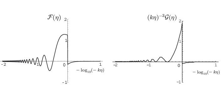
Here we show the plots of the window functions ${\cal F}(\eta)$ and ${\cal G}(\eta)/{\eta}^{3}$ in FIG. 1. FIG. 1 tells that we have only to consider the contribution from the neighborhood of the horizon crossing time. Moreover, from these window functions’ behavior, we can easily find that we may be allowed to set $\eta_{*}$ to 0 even if fall-off of $g(\eta)$ in the limit $\eta\to 0$ is not very fast, as we mentioned in Sec. IV.3.

Figure 1: The window functions ${\cal F}(\eta)$ and $(k\eta)^{-3}{\cal G}(\eta)$ as functions of $-\log(-k\eta)$.

V.2 $\phi^{\prime}=0$

When $\phi^{\prime}=0$, it seems that the solution $n^{(1)}$ diverges because $z$ vanishes, but we will see below that in fact it does not.

Using integration by parts, we can rewrite the integral $\int d\eta^{\prime}/z^{2}(\eta^{\prime})$ which appears in the Eq. (73) as

$$n^{(0)}(\eta)=-z(\eta)\int_{\eta_{\rm end}}^{\eta}\frac{d\eta^{\prime}}{z^{2}(\eta^{\prime})} = z(\eta)\int_{\eta_{\rm end}}^{\eta}d\eta^{\prime}\left\{\frac{1}{z^{\prime}(\eta^{\prime})}\frac{d}{d\eta^{\prime}}\left(\frac{1}{z(\eta^{\prime})}\right)\right\}$$ (84)

$$= -z(\eta)\left[-\frac{1}{z^{\prime}(\eta^{\prime})z(\eta^{\prime})}\right]^{\eta}_{\eta_{\rm end}}-z(\eta)\int_{\eta_{\rm end}}^{\eta}d\eta^{\prime}\left\{\frac{1}{z(\eta^{\prime})}\frac{d}{d\eta^{\prime}}\left(\frac{1}{z^{\prime}(\eta^{\prime})}\right)\right\}$$

$$= \frac{1}{z^{\prime}(\eta)}-\frac{z(\eta)}{z(\eta_{\rm end})z^{\prime}(\eta_{\rm end})}+z(\eta)\int_{\eta_{\rm end}}^{\eta}d\eta^{\prime}\left(\frac{z^{\prime\prime}(\eta^{\prime})}{z(\eta^{\prime})z^{\prime 2}(\eta^{\prime})}\right).$$

In a similar way, we also have

$$\Delta n^{(0)} = z(\eta)\int_{\eta_{\rm end}}^{\eta}d\eta^{\prime}\frac{I(\eta^{\prime})}{z^{2}(\eta^{\prime})}$$

$$= -\frac{1}{z^{\prime}(\eta)}+\frac{z(\eta)}{z(\eta_{\rm end})z^{\prime}(\eta_{\rm end})}$$

$$-z(\eta)\int_{\eta_{\rm end}}^{\eta}d\eta^{\prime}\frac{z^{\prime\prime}(\eta^{\prime})}{z(\eta^{\prime})z^{\prime 2}(\eta^{\prime})}\int_{\eta_{\rm end}}^{\eta^{\prime}}d\eta^{\prime\prime}z(\eta^{\prime\prime})n^{(0)}(\eta^{\prime\prime})+z(\eta)\int_{\eta_{\rm end}}^{\eta}d\eta^{\prime}\frac{n^{(0)}(\eta^{\prime})}{z^{\prime}(\eta^{\prime})}.$$

Here, $z^{\prime}$ and $z^{\prime\prime}/z$ can be rewritten explicitly as

$$z^{\prime} = a^{2}\left(\frac{{\phi^{\prime}}^{3}}{2{\cal H}^{2}}-2\phi^{\prime}-\frac{a^{2}V_{,\phi}}{{\cal H}}\right)~{},$$ (86)

$$z^{\prime\prime}/z = 2{\cal H}^{2}\left(1-\frac{a^{2}V_{,\phi\phi}}{2{\cal H}^{2}}-\frac{a^{2}\phi^{\prime}V_{,\phi}}{{\cal H}^{3}}-\frac{11}{4}\frac{{\phi^{\prime}}^{2}}{{\cal H}^{2}}+\frac{{\phi^{\prime}}^{4}}{4{\cal H}^{4}}\right)~{}.$$ (88)

Hence, we have $z^{\prime}\neq 0$ and $z^{\prime\prime}/z\neq\infty$ when $\phi^{\prime}=0$, as long as $V_{,\phi}\neq 0$. Therefore we find that $n^{(1)}$ doesn’t diverge even if $\phi^{\prime}$ vanishes.

Finally, it will be worth pointing out that the general slow-roll condition is even weaker than those shown in Ref. ref3 . As noted earlier, under the general slow-roll condition, the slow-roll parameters, $\delta\equiv\ddot{\phi}/H\dot{\phi}$, and $\dot{\delta}/H$ can be the same order but both are assumed to be small in Ref. ref3 . However, we can rewrite $g=\eta^{2}z^{\prime\prime}/z-2$ by using the expression for $z^{\prime\prime}/z$ given in Eq. (88) and

$$\eta^{2} = \frac{1}{{\cal H}^{2}}\left(1+2\epsilon+O(\epsilon^{2})\right),$$

where $\epsilon\equiv-\dot{H}/H^{2}$. General slow roll assumes $|g|\ll 1$. When the background scalar field motion stops ($\dot{\phi}\simeq 0$), the slow-roll parameter $\delta$ diverges. Therefore, slow-roll conditions are violated at that point. However, from Eq. (88), we can easily find that the condition $|g|\ll 1$ is maintained as far as $V_{,\phi\phi}/{H^{2}}\ll 1$ even when $\dot{\phi}\simeq 0$, namely, $\dot{\phi}\simeq 0$ does not imply the breakdown of the general slow-roll condition.

VI Summary

We have proposed a new method for a systematic derivation of formulas for the spectrum of the curvature perturbations from multi-component inflation. First we have noted that the Wronskian $W({{\mbox{\boldmath$n$}}{\mbox{\boldmath$n$}}{\mbox{\boldmath$n$}}},{{\bm{\varphi}}{\bm{\varphi}}})$ between two solutions $n$$n$$n$ and ${{\bm{\varphi}}{\bm{\varphi}}}$ of the scalar field perturbation equation in flat slicing stays constant in time. Using this fact, we have shown that the evaluation of the curvature perturbations at the end of inflation reduces to an easier problem of solving a single “decaying” mode $n$$n$$n$ backward in time from the end of inflation.

We have also shown that, for any given perturbation ${{\bm{\varphi}}{\bm{\varphi}}}$ the Wronskian $W({{\mbox{\boldmath$n$}}{\mbox{\boldmath$n$}}{\mbox{\boldmath$n$}}},{{\bm{\varphi}}{\bm{\varphi}}})$ becomes identical to $\delta N$ in the long wavelength limit by choosing an appropriate boundary condition for $({{\mbox{\boldmath$n$}}{\mbox{\boldmath$n$}}{\mbox{\boldmath$n$}}},{{\mbox{\boldmath$n$}}{\mbox{\boldmath$n$}}{\mbox{\boldmath$n$}}}^{\prime})$, where $\delta N$ is the perturbation in the $e$-folding number along the phase space trajectory of the homogeneous universe. More precisely, $\delta N$ is a perturbation in the $e$-folding number from a given point in the phase space for the homogenous universe to a point when the trajectories converge to a unique one, with $({{\bm{\varphi}}{\bm{\varphi}}},{{\bm{\varphi}}{\bm{\varphi}}}^{\prime})$ identified as the perturbation in the background phase space of spatially homogeneous fields.

Hence, with the aid of the $\delta N$ formalism SS ; ST , even if the phase space trajectories converge only after the scalar dominant phase ends, we can still evaluate the final value of the curvature perturbation by evaluating the Wronskian. Yet an open question is whether the perturbation in the true $e$-folding number, $\delta{\cal N}$, is well approximated by $\delta N$, which is determined by the dynamics of the homogeneous universe for the case with general matter fields. We plan to discuss this issue in our future publication future .

As a good example to show the efficiency of the new formulation using the Wronskian, we have presented a quick derivation of an improved general slow-roll formula, whose original form was obtained in Ref. ref3 . In Ref. ref3 or in the general slow-roll formulae given in Ref.ref4 , it was assumed that super-horizon effects are negligible. However, it was pointed out in Ref. ref2 that there are cases in which they may not be negligible at all.

The improvement that has been incoorporated for the first time in this paper is to use a systematic long-wavelength expansion for the late time evolution after horizon crossing. The matching of the two approximations, the general slow-roll approximation and the long wavelength expansion, has been easily performed by using the constancy of the Wronskian. We have shown that the formula which contains higher order corrections to the general slow-roll approximation can be obtained systematically. We have also presented an explicit power spectrum formula for the single field case. Furthermore, we have shown that our formula is valid even if the scalar field passes the point $\dot{\phi}=0$ where one of the slow-roll parameters, $\delta$, diverges ($\delta\equiv\ddot{\phi}/H\dot{\phi}\to\infty$). This fact that any special treatment is not required even if $\dot{\phi}=0$ occurs is a small but important advantage of our formulation in comparison over previous treatments Seto .

Acknowledgements

We would like to thank Takashi Nakamura for useful comments. This work is supported in part by ARCSEC funded by the Korea Science and Engineering Foundation and the Korean Ministry of Science, the KOSEF Grant (KOSEF R01-2005-000-10404-0), an Erskine Fellowship of the University of Canterbury, and JSPS Grant-in-Aid for Scientific Research, Nos. 14102004, 16740165 and 17340075.

References

• (1) H. C. Lee, M. Sasaki, E. D. Stewart, T. Tanaka and S. Yokoyama, JCAP 0510, 004 (2005) [arXiv:astro-ph/0506262].
• (2) K. Kadota and E. D. Stewart, 0307, 013 (2003) [arXiv:hep-ph/0304127].
K. Kadota and E. D. Stewart, 0312, 008 (2003) [arXiv:hep-ph/0311240].
• (3) S. M. Leach, M. Sasaki, D. Wands and A. R. Liddle, Phys. Rev. D 64, 023512 (2001).
• (4) E. D. Stewart, Phys. Rev. D 65, 103508 (2002),
J. Choe, J. O. Gong and E. D. Stewart, JCAP 0407, 012 (2004).
• (5) D. N. Spergel et al. [WMAP Collaboration], Astrophys. J. Suppl. 148 (2003) 175-194, [arXiv: astro-ph/0302209],
H. V. Peiris et al., Astrophys. J. Suppl.  148, 213 (2003) [arXiv:astro-ph/0302225].
• (6) D. N. Spergel et al., arXiv:astro-ph/0603449.
• (7) V. F. Mukhanov and P. J. Steinhardt, Phys. Lett. B 422, 52 (1998) [arXiv:astro-ph/9710038].
• (8) K. A. Malik and D. Wands, Phys. Rev. D 59, 123501 (1999) [arXiv:astro-ph/9812204].
C. Gordon, D. Wands, B. A. Bassett and R. Maartens, Phys. Rev. D 63, 023506 (2001) [arXiv:astro-ph/0009131].
D. Wands, K. A. Malik, D. H. Lyth and A. R. Liddle, Phys. Rev. D 62, 043527 (2000) [arXiv:astro-ph/0003278].
• (9) T. T. Nakamura and E. D. Stewart, Phys. Lett. B 381, 413 (1996) [arXiv:astro-ph/9604103].
• (10) D. S. Salopek, J. R. Bond and J. M. Bardeen, Phys. Rev. D 40, 1753 (1989).
• (11) N. Bartolo, S. Matarrese and A. Riotto, Phys. Rev. D 64, 123504 (2001) [arXiv:astro-ph/0107502].
• (12) J. c. Hwang and H. Noh, Phys. Rev. D 61, 043511 (2000) [arXiv:astro-ph/9909480].
• (13) A. A. Starobinsky and J. Yokoyama, arXiv:gr-qc/9502002;
J. Garcia-Bellido and D. Wands, Phys. Rev. D 52, 6739 (1995) [arXiv:gr-qc/9506050].
A. A. Starobinsky, S. Tsujikawa and J. Yokoyama, Nucl. Phys. B 610, 383 (2001) [arXiv:astro-ph/0107555].
T. Chiba, N. Sugiyama and J. Yokoyama, Nucl. Phys. B 530, 304 (1998) [arXiv:gr-qc/9708030].
• (14) D. Polarski and A. A. Starobinsky, Nucl. Phys. B 385, 623 (1992)
D. Polarski and A. A. Starobinsky, Phys. Rev. D 50, 6123 (1994) [arXiv:astro-ph/9404061].
• (15) J. Garcia-Bellido and D. Wands, Phys. Rev. D 53, 5437 (1996) [arXiv:astro-ph/9511029].
J. Garcia-Bellido and D. Wands, Phys. Rev. D 54, 7181 (1996) [arXiv:astro-ph/9606047].
• (16) D. Langlois, Phys. Rev. D 59, 123512 (1999) [arXiv:astro-ph/9906080].
• (17) M. Sasaki and E. D. Stewart, Prog. Theor. Phys. 95, 71 (1996) [arXiv:astro-ph/9507001].
A. A. Starobinsky, JETP Lett.  42, 152 (1985) [Pisma Zh. Eksp. Teor. Fiz.  42, 124 (1985)].
• (18) M. Sasaki and T. Tanaka, Prog. Theor. Phys.  99, 763 (1998) [arXiv:gr-qc/9801017].
• (19) W. I. Park, M. Sasaki, E. D. Stewart, T. Tanaka and S. Yokoyama, in preparation.
• (20) O. Seto, J. Yokoyama and H. Kodama, Phys. Rev. D 61, 103504 (2000) [arXiv:astro-ph/9911119].
• (21) H. Kodama and M. Sasaki, Prog. Theor. Phys. Suppl.  78, 1 (1984).
• (22) D. S. Gorbunov, V. A. Rubakov and S. M. Sibiryakov, JHEP 0110, 015 (2001) [arXiv:hep-th/0108017].
T. Kobayashi, H. Kudoh and T. Tanaka, Phys. Rev. D 68, 044025 (2003) [arXiv:gr-qc/0305006].
T. Kobayashi and T. Tanaka, Phys. Rev. D 71, 124028 (2005) [arXiv:hep-th/0505065].
T. Kobayashi and T. Tanaka, Phys. Rev. D 73, 044005 (2006) [arXiv:hep-th/0511186].
T. Kobayashi, arXiv:hep-th/0602168.
• (23) T. Damour and V. F. Mukhanov, Phys. Rev. Lett. 80, 3440 (1998)