The Wide Field Imager Lyman-Alpha Search (WFILAS) for Galaxies at Redshift $\sim$ 5.7

Abstract

Context. Wide-field narrowband surveys are an efficient way of searching large volumes of high-redshift space for distant galaxies.

Aims. We describe the Wide Field Imager Lyman-Alpha Search (WFILAS) over 0.74 sq. degree for bright emission-line galaxies at $z\sim 5.7$.

Methods. WFILAS uses deep images taken with the Wide Field Imager (WFI) on the ESO/MPI 2.2 m telescope in three narrowband (70 Å), one encompassing intermediate band (220 Å) and two broadband filters, $B$ and $R$. We use the novel technique of an encompassing intermediate band filter to exclude false detections. Images taken with broadband $B$ and $R$ filters are used to remove low redshift galaxies from our sample.

Results. We present a sample of seven Ly$\alpha$ emitting galaxy candidates, two of which are spectroscopically confirmed. Compared to other surveys all our candidates are bright, the results of this survey complements other narrowband surveys at this redshift. Most of our candidates are in the regime of bright luminosities, beyond the reach of less voluminous surveys. Adding our candidates to those of another survey increases the derived luminosity density by $\sim$30%. We also find potential clustering in the Chandra Deep Field South, supporting overdensities discovered by other surveys. Based on a FORS2/VLT spectrum we additionally present the analysis of the second confirmed Ly$\alpha$ emitting galaxy in our sample. We find that it is the brightest Ly$\alpha$ emitting galaxy (1 $\times\,10^{-16}$ erg s^-1 cm^-2) at this redshift to date and the second confirmed candidate of our survey. Both objects exhibit the presence of a possible second Ly$\alpha$ component redward of the line.

1 Introduction

Detections of both galaxies and QSOs at $z\,\sim\,6$ (Fan et al. 2002; Becker et al. 2001; Djorgovski et al. 2001) indicate that the Universe was largely reionised at that epoch. The recent three-year WMAP results combined with other cosmological surveys suggest an epoch of reionisation around $z\,\sim\,10$ (Spergel et al. 2006), consistent with both QSO results (Fan et al. 2002) and the epoch predicted by structure formation models (Gnedin & Ostriker 1997; Haiman & Loeb 1998). While the UV contributions of QSOs and AGN are almost certainly not responsible for reionisation (Barger et al. 2003), faint star forming galaxies need to exist in extraordinary numbers if they are to be the cause (Yan & Windhorst 2004). However, analyses of the Hubble Ultra Deep Field failed to find sufficient numbers of faint galaxies to support this idea (Bunker et al. 2004; Bouwens et al. 2005). Therefore, it is crucial to investigate what the contribution to the ionising UV flux is from young stellar populations of star forming galaxies.

Broadly speaking, two classes of star-forming galaxy dominate high redshift surveys: Lyman Break Galaxies (LBGs) and Lyman-$\alpha$ Emitters (LAEs). LBG surveys, which now number in the thousands of objects at $z$ = 3 to 5, find clumpy source distributions and a two-point angular correlation function indicative of strong clustering (Giavalisco & Dickinson 2001; Foucaud et al. 2003; Adelberger et al. 2003; Ouchi et al. 2004; Hildebrandt et al. 2005; Allen et al. 2005). LAEs also show evidence for clustering although many of the LAE surveys target fields surrounding known sources such as proto-clusters, radio galaxies and QSOs (e.g. Steidel et al. 2000; Møller & Fynbo 2001; Stiavelli et al. 2001; Venemans et al. 2002; Ouchi et al. 2005). On average, LAEs number 1.5 $\times$ $10^{4}$ deg^-2 per unit redshift down to 1.5 $\times$ $10^{-17}$ erg s^-1 cm^-2 at $z\,=\,3.4$ and 4.5 (Hu et al. 1998). Also, their consistently small size ($\lesssim$0.6 $h^{-1}$ kpc) suggests they are subgalactic clumps residing in the wind-driven outflows of larger unseen hosts (e.g. Bland-Hawthorn & Nulsen 2004). Such mechanisms provide a straightforward means of UV photon escape from the host galaxy, efficiently reionising the surrounding IGM in a way than ordinary LBGs can not.

The most efficient way to find LAEs is through imaging surveys using a combination of broad- and narrowband filters. The advent of wide field cameras has allowed systematic imaging searches that have been carried out to build up samples of candidate LAEs at high redshifts (e.g. Rhoads et al. 2003; Ajiki et al. 2003; Hu et al. 2004; Wang et al. 2005). The availability of high throughput spectrographs on 8 to 10 m-class telescopes has enabled the spectroscopic confirmation of these galaxies. Such direct imaging searches typically cover 10² – 10³ times the volume of blind long-slit spectroscopic searches (e.g. Table 4 in Santos et al. 2004). Furthermore, candidates from narrowband surveys always have an identifiable emission feature that is well separated from sky lines courtesy of the filter design. This is in contrast to other methods, including the widely-used “dropout” technique (e.g. Steidel et al. 1999).

The narrowband filter design leads to a higher candidate LAE selection efficiency than other techniques. The only way to secure the identification of the emission line is spectroscopic follow-up. The most common low redshift interlopers are the emission line doublets of [O ii] $\lambda\lambda$3726,3728 and [O iii] $\lambda\lambda$4959,5007. These can be identified by obtaining spectra with a resolution $R\gtrsim 1500$ to separate the line pair. Other emission lines, such as H$\alpha$ and H$\beta$, can be identified by neighbouring lines. The narrowband technique has been successfully applied by many authors in order to discover galaxies at redshift 5$-$6 (e.g. Ajiki et al. 2003; Maier et al. 2003; Rhoads et al. 2003; Dawson et al. 2004; Hu et al. 2004) and to locate galaxies at redshift 6$-$7 (Cuby et al. 2003; Kodaira et al. 2003; Stanway et al. 2004). Likewise, we employ the narrowband technique in the Wide Field Imager Lyman-Alpha Search (WFILAS) to find galaxies at $z\sim 5.7$. In Paper I in this series (Westra et al. 2005), we described a compact LAE at $z=5.721$ discovered by our survey.

In this Paper, we describe the survey design and sample analysis of WFILAS. In Sect. 2 we describe the scope of the survey and the observing strategy. The data reduction is described in Sect. 3. Section 4 outlines the candidate selection and Sect. 5 outlines sample properties and comparison to other surveys. We discuss the spectroscopic follow-up of two candidates in Sect. 6. Throughout this paper we assume a flat Universe with $(\Omega_{\rm m},\Omega_{\Lambda})=(0.3,0.7)$ and a Hubble constant $H_{0}=70$ km s^-1 Mpc^-1. All quoted magnitudes are in the AB system (Oke & Gunn 1983).

2 WFILAS Survey Design and Observations

Survey	Fields	Total Area	Narrowband	Filter	Co-moving	Narrowband Detection
		(sq. degree)	Filters	Width (Å)	Volume (Mpc3)	Limit ($\mu$Jy)
LALA (Rhoads & Malhotra 2001)	1	0.19	2	75	0.2$\times$106	0.41
CADIS (Maier et al. 2003)	4	0.11	8$-$9	20	0.04$\times$106	3.33
A03 (Ajiki et al. 2003)	1	0.26	1	120	0.2$\times$106	0.14
SSA22 (Hu et al. 2004)	1	0.19	1	120	0.2$\times$106	0.30
WFILAS (this paper)	3	0.74	3	70	1.0$\times$106	1.06–1.74

Table 1: Narrowband surveys for Ly$\alpha$ at $z=5.7$

Figure 1: Filter set used for the WFILAS Survey. a) The broadband $BR$ and intermediate $M_{815}$ (815/22 nm) passbands. b) The $M_{815}$ intermediate passband (solid line) and three purpose-built narrowbands $N_{810}$ (810/7), $N_{817}$ (817/7) and $N_{824}$ (824/7), shown over the wavelength region targeted for Ly$\alpha$ line detections. The transmission curves of the narrowband filters are for illustrative purposes only. The OH night sky line background is also shown.

The sky area surveyed by the WFILAS is $\sim$0.74 sq. degree. We observed three fields in broadbands $B$, $R$ and in an intermediate width filter centred at 815 nm encompassing three narrowband filters (Fig. 1). The adoption of an additional intermediate width filter encompassing the multiple narrowband width filters is a novel approach compared to previous narrowband surveys. The application of the intermediate band filter enables us to drastically reduce the number of spurious detections in the narrowband filters. The narrow width of the narrowband filters (FWHM = 7 nm) gives a prominent appearance to emission line objects. Furthermore, the three chosen fields are spread across the sky to enable us to average out variations in cosmic variance. Our search has covered one of the largest co-moving volumes compared to other surveys. Table 1 compares WFILAS with other published surveys.

The observations were taken with the Wide Field Imager (WFI; Baade et al. 1999) on the ESO/MPI 2.2 m telescope at the Cerro La Silla Observatory, Chile. The data were taken over 65 separate nights from 2001 January 19 to 2003 December 1. The WFI is a mosaic of eight ($4\times 2$) 2k $\times$ 4k CCDs arranged to give a field of view of 34^′ $\times$ 33^′. The pixels are 0$\aas@@fstack{\prime\prime}$238 on a side.

As WFILAS was planned as joint project of ESO Santiago and the COMBO-17 team at MPIA Heidelberg, three fields were selected to overlap with the COMBO-17 survey, i.e. their extended Chandra Deep Field South (CDFS), SGP (South Galactic Pole) and S11 fields. The coordinates of the field centres and the exposure times in each of the filters for each field are given in Table 2. All three fields are at high Galactic latitude ($|b|>54^{\circ}$) and have extinctions less than $E(B-V)$ = 0.022 mag (Schlegel et al. 1998).

Filter	Passband/	CDFS field			S11 field			SGP field
	FWHM	03h 32m 25$\aas@@fstack{s}$134			11h 42m 59$\aas@@fstack{s}$933			00h 45m 55$\aas@@fstack{s}$024
	(nm)	$-27$∘ 48′ 49$\aas@@fstack{\prime\prime}$75			$-01$∘ 42′ 46$\aas@@fstack{\prime\prime}$44			$-29$∘ 34′ 55$\aas@@fstack{\prime\prime}$05
		($a$)	($b$)	($c$)	($a$)	($b$)	($c$)	($a$)	($b$)	($c$)
Narrowband $N_{810}$	810/7	48.0	0.57	0.79	44.4	0.55	0.80	31.5	0.87	1.03
Narrowband $N_{817}$	817/7	41.1	0.55	0.79	79.9	0.53	0.92	0.0	-	-
Narrowband $N_{824}$	824/7	41.0	0.72	0.80	43.5	0.81	0.87	42.8	0.62	0.89
Mediumband $M_{815}$	815/20	52.7	0.29	0.85	33.3	0.38	0.88	18.9	0.41	0.90
Broadband $B$	458/97	5.0	0.07	1.09	9.4	0.07	0.98	10.0	0.14	1.22
Broadband $R$	648/160	15.1	0.05	0.75	21.2	0.07	0.75	21.5	0.07	0.76

Table 2: WFILAS fields, filter set exposure times and detection limits. The entries under each field heading list: (a) the total exposure time (ks), (b) the flux for a 2$\sigma$ detection on 6 pixel diameter aperture ($\mu$Jy) and (c) the final seeing (^′′), in each filter.

We employ standard broadband $B$ and $R$ filters. The intermediate band (FWHM = 22 nm) observatory filter is centred at 815 nm. The three custom made narrowband (FWHM = 7 nm) filters are centred at 810 nm, 817 nm and 824 nm. The transmission profiles of the filters are shown in Fig. 1. The intermediate and narrowband filters are designed to fit in the atmospheric 815 nm OH-airglow window, where the brightness of the sky background is low and hence favourable to detect Ly$\alpha$ emission at redshift $\sim$5.7. The data taken with the intermediate band filter confirm detections of the Ly$\alpha$ line in one of the narrowband filters. The broadband $B$ and $R$ data, which were taken from the COMBO-17 survey (Wolf et al. 2004), are used to confirm the absence of continuum blueward of the Ly$\alpha$ line and to avoid sample contamination by lower redshift emission line galaxies (e.g. H$\alpha$ at $z\sim 0.24$, or [O ii] at $z\sim 1.2$).

To establish the photometric zero-point of the intermediate and narrowband filters two spectrophotometric standard stars (LTT3218 and LTT7987; Bessell 1999) were observed.

Between 10–50 exposures were taken for each intermediate and narrowband filter for each field. The exposure times varied between 1000 and 1800 sec per frame, with a typical exposure time of around 1600 sec. All frames are background-limited despite the low night sky emission in this spectral region. The median, first and last decile of both seeing and background are given in Table 3.

Filter	No. of	Background ($\mu$Jy/$\Box$″)			Seeing (″)
	Frames	10%	50%	90%	10%	50%	90%
$N_{810}$	92	17	27	36	0.65	0.79	1.12
$N_{817}$	75	19	30	41	0.64	0.84	1.16
$N_{824}$	77	17	27	36	0.63	0.80	1.10
$M_{815}$	80	17	22	33	0.65	0.83	1.09

Table 3: The median, first and last decile of background and seeing for the WFILAS narrowband imaging for all three fields combined. One pixel corresponds to 0$\aas@@fstack{\prime\prime}$238.

3 Data Reduction

The data were processed with standard IRAF routines (MSCRED TASK) and our own specially designed scripts. The initial steps in the reduction process consist of removing the zero level offset with bias frames, normalising pixel-to-pixel sensitivity differences with twilight flatfield frames and removal of fringes with fringe frames. During these steps, the 8 CCDs that make up a single WFI image are treated independently. These processes are described in detail below.

Normally, the overscan region of the science frames can be used to remove the zero level offset. However, it was noticed that the bias frames contained significant intermediate scale structure (10-30 pixels). To remove this, bias frames were taken on every day of our observations and averaged into a bias frame for that day. In order to minimise the noise added to the data by subtracting the bias, the bias frames were smoothed by 5 pixels and 30 pixels in horizontal and vertical direction of the CCDs, respectively, and subsequently medianed. The structures are stable over periods of several months. Therefore, it was possible to use bias frames from different nights without degrading the quality of the data.

Typically, five twilight flatfield frames were taken in one night for one or more filters. The frames were medianed and the science data was divided by the median. Hence pixel-to-pixel sensitivity differences were removed. The structure in the individual flatfield frames was stable over a period of several weeks. Frames taken on different nights could thus be reused. Any differences between flatfield frames were due to the appearance or disappearance of dust features, or large scale illumination differences. The differences rarely amounted to more than a few percent.

The raw data in the intermediate and narrowband filters show fringe patterns with amplitudes of up to 10% which was only partially removed after the data had been flatfielded. To entirely remove the fringe pattern, we subtracted a fringe frame created from 10–30 science frames. The fringing is very stable over time, so we were able to use data spanning several months. Certain science frames still show fringe patterns because they are contaminated by either moonlight or twilight. Residual differences in the level of the background between the different CCDs were removed by subtracting the median background level from each CCD.

To produce the final deep images we only used images with a seeing of less than 5 pixels (= 1$\aas@@fstack{\prime\prime}$2) and without significant residual fringing. To make the combining of the images possible, we had to apply an astrometric correction based on stars from the USNO CCD Astrograph Catalogue 2 (UCAC2; Zacharias et al. 2004) in the three observed fields. The frames have a set pixel scale of 0$\aas@@fstack{\prime\prime}$238 pixel^-1 with North up and East left. The images were weighted according to their exposure time and combined using the IRAF “mscstack” routine rejecting deviant pixels. Table 2 summarises the depth, image quality and total exposure time, for each coadded frame.

4 Sample Selection and Completeness

4.1 Photometry and Noise Characteristics

Initial source catalogues were created for each of the 8 narrowband images. Each catalogue contains the photometry for the sources in all 6 filters. We used the SExtractor source detection software (version 2.3.2, double image mode; Bertin & Arnouts 1996). Sources were selected when at least 5 pixels were 0.8$\sigma$ above the noise level in the narrowband image used for detection. The photometry was measured in two apertures, 6 and 10 pixels in diameter (= 1$\aas@@fstack{\prime\prime}$4 and 2$\aas@@fstack{\prime\prime}$4, respectively). The 6 pixel aperture was used to maximise the signal-to-noise of the flux of the objects, while the larger 10 pixel aperture was used for the more accurate determination of the total flux and hence the star formation rate.

Some authors have found that SExtractor underestimates flux uncertainties (Feldmeier et al. 2002; Labbé et al. 2003). SExtractor estimates the uncertainties using various assumptions that are often not valid (e.g. perfect flatfielding, perfect sky subtraction). The pixel-to-pixel noise in our data is slightly correlated because the scatter in the counts summed in 6 pixel apertures is about 10% higher than what one would derive from the measured pixel-to-pixel RMS.

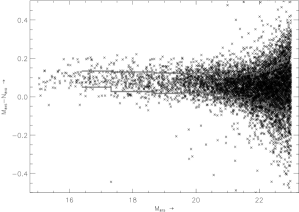
We devised a method to correct the uncertainties given by SExtractor to their true values as follows. First, sources with flux in all filters and their $M_{815}$ magnitude between 16 and 23 were selected. Sources brighter than $M_{815}$ = 16 are typically saturated, while those fainter than $M_{815}$ = 23 are incomplete (see Sect. 4.3 for a further discussion of incompleteness). The $M_{815}$–$N$ colour (where $N$ is any of narrowband filters $N_{810}$, $N_{817}$, or $N_{824}$) is the same for any flat continuum source. Therefore, the spread in the $M_{815}$–$N$ colour will be the same as the true flux uncertainty from the two contributing filters. Next, the sources were binned into 200-source bins based on their $M_{815}$ magnitude. In Fig. 2 we plot the $M_{815}$–$N$ colour versus the $M_{815}$ magnitude of one of our S11 catalogues. Mean values for the $M_{815}$–$N$ colour, $M_{815}$, $N$ magnitude and the mean of the SExtractor uncertainty were calculated for each bin. The uncertainty in the colour for each object was determined by adding the uncertainty of $M_{815}$ and $N$ in quadrature ($\sigma^{2}_{col}=\sigma^{2}_{M}+\sigma^{2}_{N}$). The interval in which 68.3% of the objects were closest to this mean colour was used to infer the actual 1$\sigma$ colour uncertainty. We assumed that the ratio between the old uncertainties $\sigma_{M}$ and $\sigma_{N}$ was the same for the new uncertainties $\sigma_{M}^{\prime}$ and $\sigma_{N}^{\prime}$. We related between the new and old uncertainty in the intermediate and narrowband flux using the function $\sigma_{\rm filter}^{\prime}=\sqrt{a^{2}+(b\sigma_{\rm filter})^{2}}$, where $a$ is the zero-offset for the uncertainty in the flux of bright sources and $b$ is the ratio between the new and old uncertainty for the flux of the faintest sources. The parameters $a$ and $b$ correspond to imperfections in the photometry and wrongly assumed background by SExtractor, respectively.

Typically, the correction factors are moderate (between $\sim$30$-$50%) for the faint sources in the catalogues. Even though the correction factors are moderate, we assume that the corrections for the uncertainties in the broadband $B$ and $R$ are irrelevant, since they are used in a different way than the intermediate and narrowband images (see Sect. 4.2).

Figure 2: $M_{815}$–$N$ colour as seen in the S11 field with the $N_{810}$ filter as the detection image. The mean colour term is $\sim$0.05. The heavy bold lines indicate the 68.3% interval of objects colours closest to the mean colour in each bin. Each bin contains 200 data points. The new uncertainty is inferred from this interval.

4.2 Selection criteria

The following four criteria were applied to select our candidate LAEs from the eight initial source catalogues:

1. the narrowband image used as the detection image must have the most flux of all the narrowband images and the source must have a 4$\sigma$ detection or better;

2. the narrowband image with the least flux needs to be a non-detection, i.e. less than 2$\sigma$;

3. there must be at least a 2$\sigma$ detection in the intermediate band image;

4. none of the broadband images, i.e. neither $B$ nor $R$, must have a detection above 2$\sigma$.

Table 2 contains the values of the 2$\sigma$ detection thresholds of the images used for the 6 pixel aperture. In total 33 candidates were selected using the above criteria. Visual inspection showed that 26 sources arose from artefacts of which the vast majority were out-of-focus ghost rings from bright stars. The final sample contains seven candidate LAEs.

We note here the importance of the usage of the intermediate band filter. If we were to reapply all the criteria except for criterion 3, i.e. we do not use the intermediate band images, we would obtain 284 candidates instead of the 33 for visual inspection.

The AB-magnitudes, derived line fluxes and luminosities for the candidates are shown in Table 6. To convert between AB-magnitudes and line flux in erg s^-1 cm^-2 we use the following relation:

$$F_{\rm line}=3\times 10^{18}\,10^{-0.4(m_{AB}+48.590)}\,\frac{\Delta\lambda}{\lambda_{c}^{2}}$$ (1)

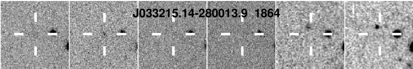
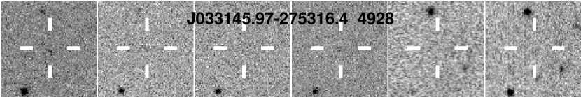
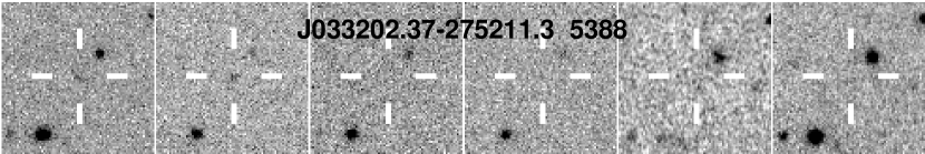
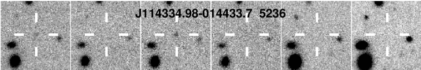
where $\Delta\lambda$ and $\lambda_{c}$ are the FWHM and the central wavelength of the narrowband filter in Å, respectively, and $m_{AB}$ the AB-magnitude of the object. In Fig. 3 the thumbnails of the seven candidate LAEs at $z\sim 5.7$ are shown. We defer a more detailed discussion about the sample properties to Sect. 5.

       $M_{815}$                              $N_{810}$                                                   $N_{817}$                                                                        $N_{824}$                                                                                              $B$                                                                                                                    $R$

Figure 3: Thumbnails of each region in which the candidate LAEs appears. The thumbnails cover a 19^′′$\times$19^′′ region with a pixel scale of 0$\aas@@fstack{\prime\prime}$238 pixel^-1 and North is up and East to the left. From left to right are the filters $M_{815}$, $N_{810}$, $N_{817}$, $N_{824}$, $B$ and $R$.

4.3 Completeness corrections

From the Hubble Deep Field (HDF) galaxy number-count data for the F814W filter (Williams et al. 1996) we computed completeness corrections for our eight source catalogues. The HDF counts are determined over the magnitude range $I_{814}$ = 22 $-$ 29, and agree well with our galaxy counts over all narrowband filters in the range $N$ = 22 $-$ 24. Figure 4 shows the counts for the F814W filter in the HDF and for the $N_{817}$ filter in the S11 field. Figure 4 also shows the linear fit used as the basis for the calculation of the detection completeness. The fit is done to the combined number count data over two intervals: $N_{817}$ = [20, 22.5], where the WFILAS counts are complete, and $I_{814}$ = [22.5, 25], where the HDF counts are linear.

Figure 4: Galaxy counts as a function of AB-magnitude for the $N_{817}$ filter in the S11 field. Plotted are the $N_{817}$ source counts of the S11 field (crosses) together with the $I_{814}$ galaxy counts of the Hubble Deep Field (squares). The solid line indicates the fitted linear relation between the magnitude and galaxy count.

Detection completeness is defined as the ratio of WFILAS sources to the number expected from the number-count relation. Figure 5 shows the derived detection completeness for each filter-field combination used for WFILAS. The differences are mainly due to unequal exposure times, although filter throughput and image quality also play a role. These could explain the overall lower sensitivity of the $N_{824}$ filter, as can be inferred from Fig. 5. Additionally, we correct for detection completeness arising due to the intermediate band selection criterion. We constructed a noise image by stacking the intermediate band images without registering. The completeness is defined as the rate of recovery of artificially inserted objects.

Figure 5: Detection of completeness as function of magnitude derived from the galaxy density-magnitude relation as described in Sect. 4. From top to bottom the CDFS, S11 and SGP fields are shown. No $N_{817}$ data are available for the SGP field.

Given the different sensitivities of each filter-field combination, we define a homogeneous subsample of our initial candidate sample, using the candidates from our four most sensitive field-filter combinations. We call this our “complete” sample (4 of the 7 LAEs; marked in Table 6), because once defined, we use the curves in Fig. 5 to correct the detected candidate numbers for incompleteness, in contrast to our initial “incomplete” sample (all 7 LAEs). The purpose of the subsample is that it lies within a uniform flux limit. Figure 5 shows that our four best filter-field combinations consist of the $N_{810}$ and $N_{817}$ filters in both the CDFS and S11 fields. These four field-filter combinations reach at least 50% completeness at $M_{\rm AB}$ = 23.38, or 5.1$\times$10^-17 erg s^-1 cm^-2. We take this as the flux limit of our complete sample. As such, the number density derived from the complete sample is a more accurate measure of the density of sources down to the nominated flux limit than the number density of the incomplete sample. Figure 6 shows the luminosity distribution of the complete sample alongside our initial candidate list, which we call the “incomplete” sample. It shows that in using completeness corrections our detected source density is up by 50%.

5 $z\sim 5.7$ Candidate LAE Catalogue

In the previous Sect. we introduced two sets of candidate LAEs: the full (but incomplete) sample of seven candidate LAEs and a subsample thereof, complete to $F_{lim}$ = 5.1$\times$10^-17 erg s^-1 cm^-2 (the complete sample). The flux limit of the incomplete sample is almost twice the limit of the complete sample (3.4$\times$10^-17 erg s^-1 cm^-2).

Figure 6: Line luminosity distribution of the candidate LAEs. Two samples are indicated: all the candidates, but not corrected for completeness (solid) and the candidates in the complete sample, i.e. candidates of the four deepest narrowband images with a magnitude cut-off at 50% completeness of the worst of these four images (dashed).

Figure 7: a) Line luminosity distribution of the complete sample of candidate LAEs (solid histograms) together with the candidates from Ajiki et al. (2003) (dashed histograms). Both samples are corrected for completeness. The errorbars are derived using Poisson statistics. Furthermore, two Schechter function fits are indicated: one to the combined WFILAS and Ajiki sample (dotted) and one to Ajiki sample only (long dashed). b) The 68.3%, 95.4% and 99.7% confidence limits for the fitting parameters $L^{*}$ and $\phi^{*}$. See text for details.

Log(L (erg s-1))	Log($\Phi$ (Mpc-3 0.1 dex-1))
42.7	-4.83${}^{+0.21}_{-0.41}$
42.8	-4.65${}^{+0.18}_{-0.30}$
42.9	-4.35${}^{+0.13}_{-0.19}$
43.0	-4.43${}^{+0.14}_{-0.21}$
43.1	-4.65${}^{+0.18}_{-0.30}$
43.2	-5.13${}^{+0.27}_{-0.87}$
43.3	-5.21${}^{+0.19}_{-0.36}$
43.4	-5.32${}^{+0.21}_{-0.44}$

Table 4: Number density of LAEs per luminosity bin as indicated in Fig. 7a.

To examine the luminosity distribution of our sample we use the Schechter function (Schechter 1976), as it is a good representation of the data at bright luminosities. From this, the luminosity density $\mathcal{L}$ of a distribution with a limiting luminosity $L_{lim}$ is given by

$$\mathcal{L}(L\geq L_{lim})=\phi^{*}L^{*}\Gamma(\alpha+2,L_{lim}/L^{*}),$$ (2)

where $\alpha$ and $\phi^{*}$ represent the slope of the faint end of the Schechter function and the normalisation constant of the galaxy density, respectively. $\Gamma$ is the incomplete gamma-function. Currently, the luminosity function for LAEs at $z\sim 5.7$ is poorly defined and authors commonly adopt either one or two of the three parameters from low redshift surveys to calculate the third.

We examine the influence of non-detections of bright ($L\gtrsim L^{*}$) LAEs for the total Ly$\alpha$ luminosity density by employing the same method as Ajiki et al. (2003), another narrowband imaging survey aimed at finding LAEs at $z\,\sim\,5.7$. In the interest of comparison, we follow Ajiki et al. exactly and adopt the Fujita et al. (2003) values for $\alpha$ (-1.53) and $\phi^{*}$ (10^-2.62 Mpc^-3). Their approach was to solve Eq. (2) for $L^{*}$, instead of fitting a Schechter function. Fixing $\phi^{*}$ and allowing $L^{*}$ and $\alpha$ to vary imposes a strong prior on the final fit, it allows us to compare directly to the results of Ajiki et al. by preserving their method. The luminosity density $\mathcal{L}$ was calculated by summing the luminosity of all candidates (corrected for completeness) and divided by the corresponding survey volume. With the given survey limits the equation can be solved for $L^{*}$. Equation (2) yields the total luminosity density when $L_{lim}=0$. We have done this for three cases: for the candidates of Ajiki et al. (case A), the complete sample of our candidates (case B) and a combined sample of these two surveys (case C). For our complete sample we derive a higher $L^{*}$ (+0.12 dex; case B) than Ajiki et al. (2003, case A) which implies an increase of the luminosity density $\mathcal{L}$ of $\sim$30%. If we scale the luminosity contribution of the candidates from Ajiki et al. to our volume and combine the two samples, $L^{*}$ is higher ($\log L^{*}=42.66$; case C). Table 7 summarises the results. Detecting LAEs of such bright luminosity at this redshift demonstrates the necessity of wide field surveys, such as WFILAS, to provide a sample of LAEs at the bright end.

Figure 8: Sky distribution of candidate line emitters per field with North up and East to the left for the a) CDFS, b) S11 and c) SGP fields. The “1”, “2” and “3” labels correspond to the $N_{810}$, $N_{817}$ and $N_{824}$ filters, respectively. The gridlines are separated by 7$\aas@@fstack{\prime}$5. In the CDFS field the Hubble Ultra Deep Field (dashed) and GOODS-S (solid) have been indicated. The confirmed $i$-drop galaxy at $z=5.78$ of Bunker et al. (2003, cross), LAEs of Ajiki et al. (2005, plus) and Stanway et al. (2004, triangle) are also indicated. In the CDFS field there seems to be a overdensity of candidates towards the southern part of the field, similar to Wang et al. (2005).

As a second approach, we tried fitting a Schechter function to the combined WFILAS and Ajiki et al. (2003) dataset, using a minimised $\chi^{2}$ fit (Fig. 7). We did not use the two lowest luminosity bins of Ajiki et al. (2003) to constrain the fit because these force the function to decline at the faint end. Instead, we set the faint end slope to $\alpha$ = $-1.53$, similar to the H$\alpha$ luminosity function at $z\sim 0.24$ from Fujita et al. (2003), on which Ajiki et al. based their work. Figure 7b shows a strong correlation between $L^{*}$ and $\phi^{*}$ due to the slow turn-over at the bright end.

From the fitting there are three results to conclude. Firstly, incorporating the four completeness-corrected WFILAS galaxies into the Ajiki et al. (2003) galaxies better constrains the bright end of the luminosity function. Furthermore, it seems that the current generation of surveys is only just reaching the volume coverage necessary to discover LAEs with $L>L^{*}$. The histogram in Fig. 7 shows a decreasing number of sources at the faint end. At face value, this could suggest that the ionising flux of the less luminous sources may be insufficient to escape the slowly expanding envelope of neutral hydrogen that surrounds the H ii region in the LAE. Consequently, the sources are undetected and the faint end of the luminosity distribution decreases. However, it is difficult to detect faint LAEs and so the possibility of detection incompleteness cannot be ruled out.

Figure 8 shows the sky distribution of our candidates in each field. All candidates but one are in the CDFS and S11 fields. The only candidate in the SGP field is brighter than the candidates in the other fields (line flux $\sim$10^-16 erg s^-1 cm^-2). The reason for this is that the $M_{815}$ filter for the SGP field has a shorter exposure time and lower signal-to-noise than the other fields.

In the CDFS field we note that our three candidates appear to be spatially clustered. Additionally, we note that the confirmed $z=5.78$ $i$-drop galaxy of Bunker et al. (2003) is at the same redshift as the WFILAS candidates in this field, just like four candidate LAEs from a narrowband survey by Ajiki et al. (2005). We did not detect these four candidates since they are fainter than the detection limits of WFILAS in this field. Wang et al. (2005) have also done a narrowband survey of the CDFS field. They also find evidence for an overdensity of $z\sim 5.7$ sources in this field. Similarly, Malhotra et al. (2005) find an overdensity at redshift 5.9 $\pm$ 0.2 in the HUDF.

6 Confirmed LAEs

In Westra et al. (2005) we reported the spectroscopic follow-up of one of the candidates, J114334.98$-$014433.7 (S11_13368 in that paper, hereafter S11_5236). It was confirmed to be a LAE at $z=5.721$. Here we present the spectral confirmation of a new candidate, J004525.38$-$292402.8 (hereafter SGP_8884), at $z=5.652$. We also show its pre-imaging and compare its Ly$\alpha$ profile to S11_5236. SGP_8884 and S11_5236 are the only two out of the seven candidates presented in this paper for which we have obtained spectra.

6.1 Spectral data reduction

Figure 9: A 38^′′ $\times$ 38^′′ region around the confirmed LAE in the SGP field. The image is created from the pre-image taken with VLT/FORS2. The image has a pixel scale of 0$\aas@@fstack{\prime\prime}$252 pix^-1. North is up and East is to the left.

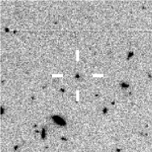
A pre-image with an intermediate band filter (FWHM = 13 nm) centred at 815 nm was taken with VLT/FORS2 on 2005 August 9. The 0$\aas@@fstack{\prime\prime}$252 pix^-1 plate scale undersamples the $\lesssim$0.5^′′stellar point spread function of the frames which were taken during excellent seeing. SGP_8884 is unresolved, implying that the FWHM of the emitting region is $\leq$2.2 kpc. A 38^′′ $\times$ 38^′′ region around the object is shown in Fig. 9.

The spectroscopy consists of four exposures of 900 s, taken on 2005 October 3 with FORS2 using the 1028z grism and a 1^′′ slit. The frames were overscan subtracted and flatfielded. They were combined by summing individual frames, thereby removing cosmic rays in the process.

The spectrum was flux calibrated using a standard star (HD 49798) taken with a 5^′′ slit and corrected for slit-loss. This was calculated assuming a Gaussian source profile with a FWHM of 0$\aas@@fstack{\prime\prime}$72 as measured from the spatial direction of the spectrum. The flux lost due to the 1^′′ slit was calculated and added to the spectrum of the object.

6.2 Line fitting

Figure 10: (Top) Flux calibrated spectrum of the confirmed candidate LAE SGP_8884, the brightest candidate in our sample. The histogram shows the observed spectrum. Indicated in grey is the best-fitting single component model after convolution with the instrumental profile. The heavy bold lines indicate three regions for which we have calculated a mean continuum. (Bottom) Residuals from the observed data minus model fit. The histograms indicate the 1$\sigma$-error spectrum from the observed data, which includes both sky- and Poisson noise. The feature at 8125 Å is due to a remnant cosmic ray from one of the spectral frames.

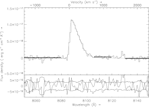
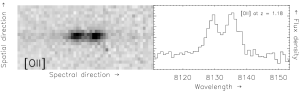
Figure 10 shows the reduced spectrum of SGP_8884 alongside its best model fit. The spectrum has an asymmetric line profile, similar to our previously confirmed candidate LAE (Westra et al. 2005). It unlikely originates from a redshifted [O ii] line at $z\sim 1.2$ because the resolution of our spectrum is high enough to resolve the [O ii] $\lambda\lambda$3726,3728. Figure 11 shows the spectrum of one such [O ii] emitter at $z=1.18$ which was included in the same observations as SGP_8884. Furthermore, we do not find any other spectral features in our spectrum, such as H$\beta$ or [N ii], which could classify the emission coming from a lower redshift galaxy. Hence, we identify the line as Ly$\alpha$ at $z=5.652$. With a total spectral line flux of (1.0 $\pm$ 0.1) $\times$10^-16 erg s^-1 cm^-2 (slit-loss corrected), SGP_8884 is the brightest LAE at redshift $\sim$5.7 to date. The line flux derived from the spectrum is consistent with the flux derived from narrowband photometry (9.5 $\pm$ 1.4) $\times$ $10^{-17}$ erg s^-1 cm^-2, which is given in Table 6. The spectral line flux corresponds to a line luminosity of $L_{\rm line}$ = 3.5 $\times$ $10^{43}$ erg s^-1 and a star formation rate of 32 $M_{\odot}$ yr^-1, using the star formation conversion rate of Ajiki et al. (2003). If we adopt $\sim$16 pixels (= 32 kpc²) as an upper limit to the size of the emitting region, we derive a star formation rate surface density of $\Sigma_{*}$ $\gtrsim$ 1 $M_{\odot}$ yr^-1 kpc^-2.

Following earlier works (e.g. Dawson et al. 2002; Hu et al. 2004; Westra et al. 2005) we fitted a single component model to the Ly$\alpha$ line SGP_8884. The model consists of a truncated Gaussian with complete absorption blueward of the Ly$\alpha$ line centre. We find an excess of flux in the observed data compared to the model around 8110 Å. This suggests the presence of a second line component redward of the main peak. To test this, we measured the mean continuum levels, both red- and blueward of the line, as well as across the red-flanking region of the line. The continuum is calculated as the weighted mean of the flux density over this region. This yields for continuum in the red-flanking region a flux density of (3.2 $\pm$ 0.8) $\times$ 10^-19 erg s^-1 cm^-2 Å^-1. Red- and blueward of the Ly$\alpha$ line the continuum is (-1.0 $\pm$ 0.8) $\times$ 10^-19 erg s^-1 cm^-2 Å^-1 and (0.9 $\pm$ 0.6) $\times$ 10^-19 erg s^-1 cm^-2 Å^-1, respectively. These continuum levels are indicated by the heavy bold lines in Fig. 10. The lower limit for the rest frame equivalent width derived from the continuum of the red flank is 46 Å. The rest frame equivalent width derived from the 2$\sigma$ upper limit of the continuum redward of the line is 125 Å.

Figure 11: (Left) Two dimensional spectrum of an [O ii] emitting galaxy at $z=1.18$ in the SGP field. (Right) The extracted one dimensional spectrum. We are able to easily resolve the [O ii] $\lambda\lambda$3726,3728 lines with the available resolution. Both spectra are background subtracted.

Figure 12: Comparison of the Ly$\alpha$ line profiles of the two WFILAS sources, SGP_8884 and S11_5236. a) Two dimensional background-subtracted spectrum of SGP_8884. b) Observed Ly$\alpha$ line (histograms) with the best-fitting one component model (grey solid line). c) Same model line profile as in b) but before convolution with the instrument profile. d) Observed data minus model fit (as plotted in b)). Also shown (histograms) is the 1$\sigma$-error spectrum from the observed data, which includes both sky- and Poisson noise. Panels e) through h) show the same for S11_5236. The horizontal axes show both the wavelength (in Å; bottom) and velocity offset from the centre of the full Gaussian of the Ly$\alpha$ line (in km s^-1; top)

Component	$\lambda_{c}$	$f_{\rm peak}$	FWHM		$\Delta v$
(1)	(2)	(3)	(4)	(5)	(6)	(7)
SGP_8884 single component
Single peak	8086.2	1.2 $\times$ 10-17	15.7	580
S11_5236 single component
Single peak	8172.2	8.3 $\times$ 10-18	13.5	495
S11_5236 double component, “broad”
Main peak	8173.1	8.0 $\times$ 10-18	11.3	413
Red peak	8184.1	1.9 $\times$ 10-18	2.3	85	+11.1	+406
S11_5236 double component, “narrow”
Main peak	8173.1	8.1 $\times$ 10-18	11.2	413
Red peak	8184.1	4.8 $\times$ 10-18	0.5	18	+11.0	+403

Table 5: Parameters for the single component model to SGP_8884 before convolution with the instrumental profile. We also include the parameters for the single component and the two double component models of the previously confirmed LAE S11_5236 (Westra et al. 2005). These parameters differ slightly from Westra et al., since we have subsequently corrected the spectrum of S11_5236 for slit-losses.
Notes: (1) component of the fit, (2) central wavelength of the fitted component in Å, (3) peak flux density in erg s^-1 cm^-2 Å^-1, (4) and (5) FWHM of full Gaussian of the profile in Å and km s^-1, respectively, (6) and (7) velocity shift of the second component in Å and km s^-1.

To see if the excess of flux in the red flank of the Ly$\alpha$ line can be explained by an outflow, we fit a second Gaussian component to the spectrum of SGP_8884, as we did to the spectrum of S11_5236 in Westra et al. (2005). This yields an extremely faint and broad second component ($f_{\rm peak}$ $\sim$5 $\times$ 10^-19 erg s^-1 cm^-2 Å^-1 and FWHM $\sim$1700 km s^-1). The precise parameters for the red component are difficult to constrain given its faint and broad profile. The parameters from the single component model for SGP_8884 and the single and double component models for S11_5236 are given in Table 5.

6.3 Discussion/Comparison

The Ly$\alpha$ emission we see is due to intense star formation rates synonymous with local starburst galaxies. Star formation rates per unit area in excess of 0.1 $M_{\odot}$ yr^-1 kpc² are prone to produce large scale outflows of neutral hydrogen from a galaxy, powered by the supernovae and stellar winds of massive stars (Heckman 2002). The most efficient way for Ly$\alpha$ to escape from the compact star forming regions is due to scattering of the photons by the entrained neutral hydrogen (Chen & Neufeld 1994). The kinematics and orientation of the outflowing neutral hydrogen can alter the Ly$\alpha$ profile by absorbing photons bluer if along the line of sight, or backscattering redder than Ly$\alpha$ if behind and receding (e.g. Dawson et al. 2002). Ly$\alpha$ emission can also arise when large scale shocks from starburst winds impinge on clumps ($\sim$100 pc) of condensed gas accreting onto the halo (Bland-Hawthorn & Nulsen 2004).

Most examples of asymmetric Ly$\alpha$ emission at $z\sim 6$ show an extended tail implying backscattering over a fairly wide range of velocities beyond the central Ly$\alpha$ emission (e.g. Fig. 9 of Hu et al. 2004). The limiting physical size of SGP_8884 (FWHM $<$ 2.2 kpc) is consistent with the scale of emitting regions in the local starburst galaxy M82 which span 0.5 to 1 kpc (Courvoisier et al. 1990; Blecha et al. 1990). This, and the scale of its outflow, make it fairly typical of both the starbursting sources seen at $z\sim 6$ and their local counterparts.

The tentative discovery of a second component in S11_5236 (Westra et al. 2005) could be explained by either an expanding shell of neutral hydrogen (Dawson et al. 2002; Ahn et al. 2003), or by infall of the IGM onto the LAE (Dijkstra et al. 2005). The flux of the intrinsic Ly$\alpha$ line depends heavily on the model. It is suggested that the total intrinsic Ly$\alpha$ flux emerging from these sources is underestimated by an order of magnitude (e.g. Dijkstra et al.). Therefore, the star formation rates derived from the observed Ly$\alpha$ lines could be heavily underestimated.

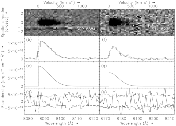
Figure 12 shows a comparison between the line profiles of the two LAEs discovered with WFILAS. S11_5236 differs from SGP_8884 in that a clear peak, $\sim$20 $-$ 90 km s^-1 wide, is seen $\sim$400 km s^-1 redward of Ly$\alpha$ (Westra et al. 2005). The red component is narrower ($\sim$15%) and relatively stronger than SGP_8884. The difference in the width of the red component is even more pronounced ($\sim$30%) when we compare the main peak of the two-component fits to the spectrum of S11_5236 to the single peak of the one-component fits to the spectrum of SGP_8884. This can clearly be seen in panels a and e of Fig. 12.

Ultimately, such outflows are thought to be responsible for the chemical enrichment of the IGM by $z\sim 6$ (Aguirre et al. 2001). Outflows are a process facilitating the escape of UV photons, which are the origin for the UV background (Madau et al. 1999).

7 Summary

In this paper we have presented the Wide Field Imager Lyman-Alpha Search (WFILAS), which uses a combination of narrow-, intermediate and broadband filters on the ESO/MPI 2.2 m telescope to search for LAEs at redshift $z\sim 5.7$. This search has resulted in seven bright ($L$ $\geq$1.1$\times$10⁴³ erg s^-1) candidate galaxies across three fields spanning almost 0.8 sq. degree.

Most of our candidates are in the regimes of bright luminosities, beyond the reach of less voluminous surveys. Adding our candidates to those of earlier such surveys results in an integrated luminosity density $\mathcal{L}$ $\sim$30% higher than found by such surveys alone. We also find potential clustering in our CDFS field, supporting overdensities discovered by other surveys. Spectroscopic follow-up for confirmation in this area will be crucial.

Two candidates have been confirmed to be LAEs at $z\sim 5.7$ by means of spectroscopy. One of these galaxies is the brightest LAEs at this redshift. The broad, asymmetric profiles of the Ly$\alpha$ line of both objects are consistent with neutral hydrogen backscattering of a central starbursting source.

SExtractor ID	Object ID	$B$	$R$	$M_{815}$	$N_{810}$	$N_{817}$	$N_{824}$	Line flux	Luminosity
								(10-17 erg s-1 cm-2)	(1043 erg s-1)
CDFS_1864	J033215.14-280013.9	$>$26.25	$>$26.56	24.72 $\pm$ 0.46	23.14 $\pm$ 0.26	$>$24.27	$>$23.93	6.5 $\pm$ 1.5	2.3 $\pm$ 0.5
CDFS_4928	J033145.97-275316.4	$>$26.25	$>$26.56	24.59 $\pm$ 0.41	23.38 $\pm$ 0.32	24.11 $\pm$ 0.47	23.61 $\pm$ 0.41	5.2 $\pm$ 1.6	1.8 $\pm$ 0.5
CDFS_5388	J033202.37-275211.3	$>$26.25	$>$26.56	24.70 $\pm$ 0.45	23.32 $\pm$ 0.31	$>$24.27	$>$23.93	5.5 $\pm$ 1.5	1.9 $\pm$ 0.5
S11_5236	J114334.98-014433.7	$>$26.63	$>$26.59	24.31 $\pm$ 0.42	$>$24.13	23.05 $\pm$ 0.18	$>$23.74	7.0 $\pm$ 1.2	2.5 $\pm$ 0.4
S11_8921	J114218.90-013544.6	$>$26.63	26.38 $\pm$ 0.45	23.88 $\pm$ 0.28	23.98 $\pm$ 0.47	23.41 $\pm$ 0.26	$>$23.75	5.0 $\pm$ 1.2	1.8 $\pm$ 0.4
S11_10595	J114312.46-013049.6	$>$26.63	$>$26.60	24.44 $\pm$ 0.47	$>$24.13	23.52 $\pm$ 0.28	$>$23.75	4.5 $\pm$ 1.2	1.6 $\pm$ 0.4
SGP_8884	J004525.38-292402.8	$>$26.07	$>$26.41	23.33 $\pm$ 0.20	22.73 $\pm$ 0.16		$>$24.06	9.5 $\pm$ 1.4	3.3 $\pm$ 0.5

Table 6: The candidate list of the WFILAS survey after the selection as described in Sect. 4. From left to right are the object name, the $B$, $R$, $M_{815}$, $N_{810}$, $N_{817}$ and $N_{824}$ AB-magnitudes, line flux calculated from the narrowband magnitude in which the object was detected and line luminosity. For all measurements less than $2\sigma$ the $2\sigma$ upper limit has been given.

	$\alpha$	$\log\phi^{*}$	$\log L^{*}$	$\log L_{lim}$	log $V$	$\log\mathcal{L}$	Comment
		Mpc-3	erg s-1	erg s-1	Mpc3	erg s-1 Mpc-3
Case A	–	–	–	42.85	5.26	39.04	Sum of the candidates from Ajiki et al. (2003)
	-1.53	-2.62	42.61	42.85	5.26	39.04	Integrated luminosity function down to Ajiki et al. (2003) survey limit (7.0$\times$1042 erg s-1)
	-1.53	-2.62	42.61	–	–	40.27	Integration of the entire luminosity function
Case B	–	–	–	43.26	5.71	38.36	Sum of the candidates from completeness corrected WFILAS sample
	-1.53	-2.62	42.74	43.26	5.71	38.36	Integrated luminosity function down to the limit of the completeness corrected sample (1.8$\times$1043 erg s-1)
	-1.53	-2.62	42.74	–	–	40.39	Integration of the entire luminosity function
Case C	–	–	–	42.85	5.84	39.19	Sum of the combined WFILAS and Ajiki et al. (2003) samples low luminosity corrections
	-1.53	-2.62	42.66	42.85	5.84	39.19	Integrated luminosity function down to Ajiki et al. (2003) survey limit (7.0$\times$1042 erg s-1)
	-1.53	-2.62	42.66	–	–	40.32	Integration of the entire luminosity function

Table 7: Calculation of the Schechter function parameter $L^{*}$ and luminosity density $\mathcal{L}$ according to Ajiki et al. (2003) for their sample, our complete sample and the combination of the two. For each sample the luminosity density has been derived from the sum of the candidate luminosities divided by the corresponding survey volume. Then Eq. (2) was solved for $L^{*}$, with given $\alpha$ and $\phi^{*}$ from Ajiki et al. (2003). Finally, the entire luminosity function was integrated to give the final luminosity density.