Global properties of the HI high velocity sky

Abstract

Context. Since 1973 it is known that some H i high velocity clouds (HVCs) have a core-envelope structure. Recent observations of compact HVCs confirm this but more general investigations have been missing so far.

Aims. We study the properties of all major HVC complexes from a sample compiled 1991 by Wakker & van Woerden (WvW).

Methods. We use the Leiden/Argentine/Bonn all sky 21-cm line survey and decompose the profiles into Gaussian components.

Results. We find the WvW line widths and column densities underestimated by $\sim 40$%. In 1991 these line widths could not be measured directly but had to be estimated with the help of higher-resolution data. We find a well defined multi-component structure for most of the HVC complexes. The cold HVC phase has lines with typical velocity dispersions $\sigma=3$ km s^-1and exists only within more extended broad line regions, typically with $\sigma=12$ km s^-1. The motions of the cores relative to the envelopes are characterized by Mach numbers $M=(v_{core}-v_{envelope})/\sigma_{envelope}\sim 1.5$. The center velocities of the cores within a HVC complex have typical dispersions of 20 km s^-1. Remarkable is the well defined two-component structure for some prominent HVC complexes in the outskirts of the Milky Way: Complex H lies approximately in the galactic plane, and the most plausible distance estimate of $R\sim 33$ kpc places it at the edge of the disk. The Magellanic Stream and the Leading Arm (complex EP) reach higher latitudes and are probably more distant, $R\sim 50$ kpc. There might be some indications for an interaction between HVCs and disk gas at intermediate velocities. This is possible for complex H, M, C, WB, WD, WE, WC, R, G, GCP, and OA, but not for complex A, MS, ACVHV, EN, WA, and P.

Conclusions. The line widths, determined by us, imply that estimates of HVC masses, as far as derived from the WvW database, need to be scaled up by a factor 1.4. Correspondingly, guesses for the external pressure of a confining coronal gas need to be revised upward by a factor of 2. The HVC multi-phase structure implies in general that currently the halo pressure is significantly underestimated. In consequence, the HVC multi-phase structure may indicate that most of the complexes are circum-galactic. HVCs have turbulent energy densities which are an order of magnitude larger than that of comparable clumps in the Galactic disk.

1 Introduction

Forty years after the discovery of high velocity clouds (HVCs) outside the disk of the Milky Way (Muller et al., 1963) the nature of these distinguished objects has still remained a mystery. Large quantities of data have been collected since then and numerous explanations for their origins have been proposed, we refer to the review by Wakker & van Woerden (1997) and volume 312 of the Astrophysics and Space Science Library, dedicated to the HVC phenomenon (van Woerden et al., 2004a). An outstanding contribution and one of the roots for our present understanding of the structure and distribution of HVCs on large scales is the catalog of individual HVCs by Wakker & van Woerden (1991) (hereafter WvW).

Our contribution to this topic, presented here, is based on the Leiden/Argentine/Bonn (LAB) H i line survey (Kalberla et al., 2005). This new survey combines the southern sky survey of the Instituto Argentino de Radioastronomìa (IAR) (Bajaja et al., 2005) with an improved version of the Leiden/Dwingeloo Survey (LDS) (Hartmann & Burton, 1997). Currently this is the most sensitive Milky Way H i line survey with the most extensive coverage both spatially and kinematically. Naturally, since H i provides the main emission line of HVCs, one can hope that this survey may provide some new insights to the HVC phenomenon. A comparison to previous results, in particular to those by Wakker & van Woerden (1991), appears mandatory.

The LDS survey, covering declinations $\delta\ga-30\hbox{${}^{\circ}$}$, is available since 1997. Its velocity coverage of $-450<v<400$ km s^-1is large enough to study most of the high velocity gas in the Milky Way, only complex EN is known to have H i emission at $v<-450$ km s^-1. For HVC research the LDS was predominantly used for large scale investigations, e.g. searches for signs of interaction between HVCs and disk gas (Pietz et al., 1996; Brüns et al., 2000), a search for soft X-ray emission associated with prominent high-velocity-cloud complexes, (Kerp et al., 1999) and a proposal to explain HVCs as building blocks of the Local Group (Blitz et al., 1999). A new class of compact isolated HVCs has been detected by Braun & Burton (1999) and studied in more detail by de Heij et al. (2002b, c). An advantage of the LDS over older surveys was the improved velocity resolution, also the better spatial coverage without gaps. Most of the instrumental errors originating from the side-lobes of the antenna diagram have been removed. Still, some instrumental problems are noticeable at a level $T_{B}\la 0.1$K. Wakker (2004) claims in addition sensitivity limitations and discrepancies when comparing maps from the LDS with those derived from the Hulsbosch & Wakker (1988) database.

The LAB survey improves on the LDS, residual limitations have been discussed by Kalberla et al. (2005) and are not expected to be severe enough to cause notable problems. Still, maps of HVCs based on the LAB survey (Kalberla et al., 2005, see e.g. Figs. 4&5) do not differ significantly from LDS maps and the discrepancies discovered by Wakker (2004) remain to be explained.

In Sect. 2 we compare column densities derived from the LAB survey with those from Wakker & van Woerden (1991). We find systematical deviations in line widths listed by Wakker & van Woerden (1991) and those derived from the LAB as second moments of the HVC line emission. To study the discrepancies in more detail we use in Sect. 3 a Gaussian decomposition. We find for most of the HVC complexes clear indications for a multi-phase structure and discuss the properties of individual HVC complexes in Sect. 4 in some detail. There are hints for a possible interaction between HVCs and gas closer to the Milky Way, described in Sect. 5. In Sect. 6 we discuss properties of the multi-phase HVC gas. Our summary is in Sect. 7.

2 Basic statistical investigations

We use measurements and cloud assignments based on the observation by Hulsbosch & Wakker (1988) and Bajaja et al. (1985). The database in form of a table containing HVC positions, velocities, line widths, and peak temperatures, was prepared by Wakker (1990) and used by Wakker & van Woerden (1991) for a classification of HVCs into complexes and populations. Also the review by Wakker & van Woerden (1997) is based on this table. We therefore use the term “WvW database” or “WvW table” for reference.

2.1 Peak temperatures and calibration

For each entry in the WvW database we compare first the peak temperature at a given center velocity $v_{c}$ with the temperature of the LAB profile at the same velocity. Unfortunately, due to differences in sampling, only a small number of LAB profiles agree in position exactly with those entering the more coarsely sampled material used by Wakker & van Woerden (1991). To overcome this discrepancy, a mean LAB profile was derived by convolving the original observed LAB database with a Gaussian smoothing kernel of 0.3^∘  FWHM. This degrades the angular resolution for the LAB data slightly (10%). Next we took the difference in velocity resolution into account. The spectra available for the WvW catalog had 8 km s^-1  velocity resolution, and were smoothed to 16 km s^-1  before their analysis, while the LAB survey was observed with a resolution of 1.03 km s^-1. A direct comparison of the peak temperatures would be affected by resolution and instrumental noise, we therefore calculate mean temperatures from the LAB spectra by averaging 15 channels, corresponding to the velocity resolution of 16 km s^-1  of the spectra used by WvW. Comparing the derived peak temperatures leads to an excellent agreement. On average, the peak temperatures deviate by 0.9% only, indicating a perfect consistent calibration.

2.2 Direct comparison of column densities

Next we compare the derived column densities. From the interpolated LAB profile we determined the H i column density for each HVC component in the WvW list by integrating the LAB profile within the velocity range $v_{c}-\Delta v<v<v_{c}+\Delta v$, where $v_{c}$ and $\Delta v$ are the LSR component velocity and its associated FWHM velocity width according to the WvW table. For a Gaussian distribution 98% of the line integral is expected in this range.

Fig. 1 shows a comparison between column densities, derived from the LAB, with those from the WvW catalog. We find the regression $N_{H}({\rm LAB})=1.37\cdot N_{H}({\rm WvW})$ (lower dotted line). Despite a large scatter, there is at large column densities a clear deviation from the expected relation (solid line). At low column densities the scatter gets worse, apparently indicating on average $N_{H}({\rm LAB})<N_{H}({\rm WvW})$. The latter effect might be caused by increasing uncertainties for component parameters at low column densities, leading to a systematic mismatch for the redetermined LAB parameters.

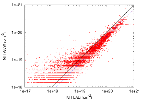
Figure 1: H i column densities from the WvW database in comparison with column densities determined from the LAB survey. The solid line indicates the expected correlation, the lower dotted line (blue) $N_{H}$(LAB) = 1.37 $N_{H}$(WvW).

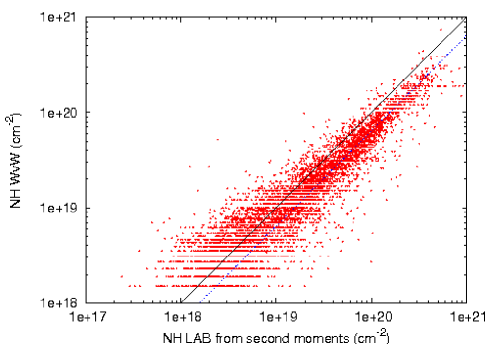
Figure 2: H i column densities from the WvW database in comparison with column densities determined from the LAB survey after a redefinition of the HVC component widths. In this case the LAB survey was smoothed to a resolution of $1.5\hbox{${}^{\circ}$}$. The solid line indicates the expected correlation, the lower dotted line (blue) the correlation $N_{H}$(LAB) = 1.55 $N_{H}$(WvW).

2.3 Column densities from first and second moments

To investigate the problem in more detail, we refined the determination of component center velocities and dispersions for the LAB profiles. We use peak velocities $v_{p}$, redetermined from the LAB, and line widths $\Delta v$ from the WvW table. Next we derive for the range $v_{p}-\Delta v<v<v_{p}+\Delta v$ a first guess for the first and second moments of each HVC component. Next we replace $v_{p}$ with the first moment and $\Delta v$ with the FWHM derived from the second moment and reiterate the last step to obtain the final component velocity $v_{cL}$ and its FWHM width $\Delta v_{cL}$. We then use the velocity range $v_{cL}-\Delta v_{cL}<v<v_{cL}+\Delta v_{cL}$ for a new determination of LAB column densities. For 85% of all components in the WvW list we find this way components with well defined peak temperatures, first, and second moments. To improve the signal-to-noise ratio of the LAB survey we repeated the whole procedure for different spatial resolutions of the LAB profiles. We used alternative Gaussian smoothing kernels with FWHM of 1.0^∘  and 1.5^∘  and derive $N_{H}({\rm LAB})\sim 1.55\leavevmode\nobreak\ N_{H}({\rm WvW})$. Fig. 2 displays WvW and LAB column densities for a 1.5^∘  smoothing kernel.

Improving our search algorithm for HVCs with respect to the procedure described in Sect. 2.2 leads to a significant decrease of the scatter at low column densities. Comparing the different resolutions we find that the total scatter, however, increases with increasing LAB beam width. Spatial fluctuations in the HVC emission may be responsible for this effect. An increasing mismatch of the beam shapes would cause increasing discrepancies of the derived column densities.

When comparing the derived center velocities $v_{cL}$ with velocities $v_{c}$ from the WvW catalog, we find RMS deviations between 7.7 km s^-1  (1.5^∘  smoothing kernel) and 9 km s^-1  (0.3^∘  kernel). This is about half of the FWHM velocity resolution and twice the expected uncertainties of 4 km s^-1  (Hulsbosch & Wakker, 1988). The deviations are purely statistical and without any bias. The average component velocities agree within 0.01 km s^-1. Spectrometer problems as a reason for the column density discrepancies can therefore be excluded.

A major restriction of our analysis is that our component search algorithm diverges for 15% of the WvW components. Discrepant component parameters might have two reasons. The signal in the LAB survey may be too weak. This applies to 3% of all cases. In most cases, 12%, we found a profile structure that is too complicated for our approach. We demand in any case $|v_{cL}-v_{c}|<\Delta v$, the refined component velocity has to be within the limits of the WvW catalog. For a line width of 20 km s^-1  this means a 2.5 sigma deviation, a rather stringent limit.

Among those LAB profiles that fail to have HVC emission at a four to five sigma level at positions where WvW components are present we visually inspected 115 of the most serious cases. In 29 cases we find some emission at velocities deviating significantly from the WvW catalog but in 74 cases we do not detect any significant HVC emission in the LAB profiles. For the remaining 12 cases the situation was unclear, the LAB baselines might have been affected by interference.

2.4 Comparison of line widths

Searching for a reason for the discrepancies in the derived column densities we can exclude calibration and spectrometer problems, but a discussion of the linewidth remains to be done. Fig. 3 displays a comparison of velocity dispersions, which implicitly have been used to calculate the column densities in Fig. 2. To derive this Fig. we degraded the spatial resolution of the LAB to 1.5^∘. Our intention was to improve the sensitivity of our analysis without degrading the velocity resolution. In turn, uncertainties for the derived second moments of the HVC components depend on their widths. Components with dispersions $\sigma\ga 8.5$ km s^-1  are in sensitivity equivalent to the components from the Wakker & van Woerden (1991) database. This, however, applies to more than 90% of all cases, the huge scatter in Fig. 3 is significant. In particular, we note that 87% of all WvW components have a dispersion of 8.5 km s^-1. Most of our second moments are significantly larger. Fig. 3 shows this effect barely because of the crowding of the WvW components with a dispersion of 8.5 km s^-1.

Line widths in the WvW database were based on observations with a poor velocity resolution. The spectra were hanning smoothed to 16.5 km s^-1resolution and the data quality did not allow to distinguish lines of 25 km s^-1FWHM or narrower. As estimates were needed (Wakker, private communication), these were based mostly on the widths of the profiles in cloud envelopes that were found in several 1970s papers, such as Cram & Giovanelli (1976); Giovanelli & Haynes (1976, 1977); Davies et al. (1976). Originally Hulsbosch & Wakker (1988) have chosen a line width of 25 km s^-1FWHM but Wakker & van Woerden (1991) revised this to 20 km s^-1, corresponding to a dispersion of $\sigma=8.5$ km s^-1, the value we use here.

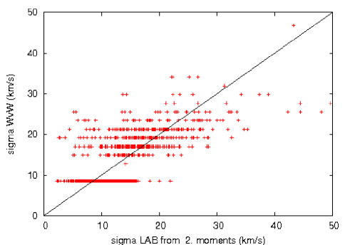
Figure 3: Estimated velocity dispersions from the WvW database in comparison with dispersions determined from the LAB survey using second moments. In 87% of the WvW database the estimate $\sigma=8.5$ km s^-1  (FWHM = 20 km s^-1) was used, too crowded to be resolved in this plot.

We conclude that the scatter in Fig. 3, independent from the signal-to-noise level of the HVC component, originates predominantly from uncertainties in estimating the line width. The bias $N_{H}$(LAB) $\sim 1.5N_{H}$(WvW), visible in Fig. 1 & 2 would be explainable as a general bias of the the narrowest lines which are most frequent in the WvW table.

We verified, whether non-Gaussian line shapes might affect the linewidth determination. Using channels centered on the component velocity $v_{c}$ with a window given by the FWHM $\Delta v$ on both sides of the line should, in case of a Gaussian component, lead to 98% of the line integral. Broadening the window should essentially be without significant effects. We tested this assumption, increasing the window by 10%. As a result the line integrals increase 2.7%, but only 1% is expected. We conclude that HVC components, on average, must have line shapes that deviate significantly from single component Gaussians. As an additional test we have split the HVC components at their center velocities in two parts. Both subcomponents were integrated separately. In this case the discrepancies increased by another factor of two, indicating that a significant fraction of the HVC line components must be asymmetric. From high resolution observations it is known since long that HVC lines are asymmetric (e.g. Giovanelli et al. (1973), see also the discussion in Sect. 2.7 of Wakker & van Woerden (1997)). Apparently we recovered this general property of HVCs on a broader basis. Some uncertainties are expected if column densities are calculated by simply multiplying the peak of the line emission with a measure of the component width.

3 Gaussian decomposition

We decomposed all profiles of the LAB survey into Gaussian components. The procedure is equivalent to the decomposition of the LDS described by Haud (2000). A detailed statistical analysis and a classification of Gaussian components concerning possible spurious components is given by Haud & Kalberla (2006). A publication of the database is in preparation. Based on the WvW database we searched for components within the LSR velocity range $v_{c}-\Delta v<v<v_{c}+\Delta v$. All positions within the HVC complexes have been selected by interpolating the WvW HVC distribution. According to the predefined velocity range we rejected components with $|v|<90$ km s^-1, exceptions will be discussed in Sects. 4 to 6. Also components with $\sigma>50$ km s^-1  or $\sigma<0.5$ km s^-1  have been rejected because they most probably represent spurious signals due to baseline deficiencies or single-channel interference spikes.

3.1 Line width distribution

The frequency distribution of derived LAB Gaussian components with respect to their velocity dispersions is shown in Fig. 4. The upper distribution shows a summary over all 23070 components found at 17336 positions while the lower dotted distribution is restricted to those 13221 positions where only a single Gaussian component was found. Clearly, broad lines dominate the distribution, in particular for single component features. The first moment of the upper distribution is at 10.7 km s^-1. Narrow components with typical dispersions of 3 km s^-1  are most significant at positions where a multi-phase structure is found.

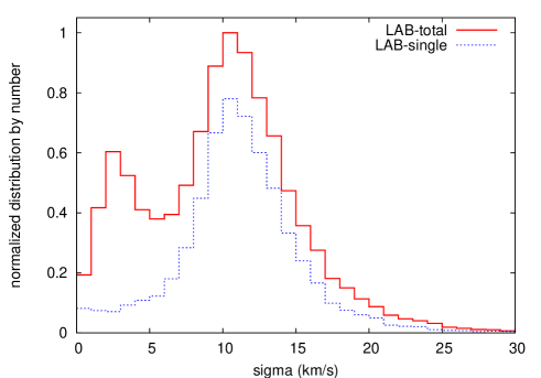
Figure 4: Frequency distribution of component line widths. The solid line is the histogram derived after Gaussian decomposition of the LAB survey. The lower dotted line represents the subset of single component HVC profiles, using the same normalization.

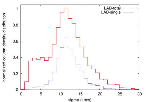
Figure 5: Distribution of column densities as function of linewidth. The solid line is the histogram derived from the LAB survey. The lower dotted line represents the subset of single component HVC profiles, using the same normalization.

Fig. 5 shows how the Gaussian components contribute to the observed column densities. At positions having only a single component (lower dotted line) we barely find narrow lines. 62% of the total column density is associated with multi-component structures, but these cases are observed only at 24% of all positions. Broad lines dominate also the multi-component distribution, 75% of the multi-component HVC emission is in broad lines. We call therefore the broadest line of a multi-component set the “primary” component. This definition allows us to differentiate Gaussian components according their line widths. The narrow lines are the “secondary” components. If several secondary components are found we sort according to their velocities. Components with the least deviations in velocity are considered first.

The secondary components contain in most cases less column density than the primary ones. Nevertheless, secondary components are important. They contain only 21% of the total observed H i column density but are tracers for regions with significant enhanced HVC emission, resembling “H i icebergs”. The first moment of the total observed distribution (upper curve in Fig. 5) is $\sigma=11.8$ km s^-1. For those spectra that have single HVC components only (lower curve in Fig. 5) we find a first moment $\sigma=11.1$ km s^-1.

First evidence for a multi-component velocity structure of some HVCs has been given by Giovanelli et al. (1973), a more detailed analysis was provided by Cram & Giovanelli (1976). These authors used the NRAO 140-foot telescope to search about 100 directions with local concentrations of HVC emission for multi-component features. They found evidence for two well defined velocity domains, one at FWHM of about 23 km s^-1  ($\sigma\sim 10\leavevmode\nobreak\$ km s^-1) and one at FWHM of about 7 km s^-1  ($\sigma\sim 3$ km s^-1). Broad components, called by us “primary”, correlate with more extended regions (envelopes). Narrow lines, “secondary” components, correlate with small, bright condensations (cores) and with larger column densities. This finding resembles the well established two-component structure of the neutral interstellar medium.

Our results are in excellent agreement with Cram & Giovanelli (1976), except that we find somewhat larger line widths. A reason may be that Cram & Giovanelli (1976) disregarded components associated with line wings, excluding broad lines with $\sigma>13$ km s^-1  from their analysis. Lockman et al. (2002), pointing the NRAO 140-foot telescope to 860 random positions, found a distribution very similar to our single component distribution, with median dispersion of 12.9 km s^-1. Narrow lines may be underrepresented in their analysis due to limitations in velocity resolution of 5 km s^-1  FWHM. Burton et al. (2001) derived a typical width of $\sigma\sim 10.6$ km s^-1  from Arecibo observations of compact high velocity clouds. There might be a tendency that the component widths decrease with decreasing beam width but $11\la\sigma\la 13$ km s^-1  appears to be a typical dispersion, our result is in any case consistent.

87% of the WvW database has $\sigma=8.5$ km s^-1  (FWHM = 20 km s^-1), quite different from our results. Comparing the line widths, we find a typical ratio $\sigma({\rm LAB})/\sigma({\rm WvW})\sim 1.4$. Recalling that we found an excellent agreement in the observed peak temperatures, we explain the systematic $N_{\rm HI}$  discrepancies discussed in Sect. 2 (see also Figs. 1 and 2) as due to a general bias in the WvW line widths.

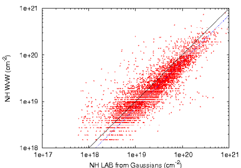
Figure 6: H i column densities from the WvW database in comparison with column densities determined from the LAB survey after Gaussian decomposition. For each position from the WvW table the nearest LAB position was searched for. The solid line indicates the expected correlation, the lower dotted line (blue) the correlation $N_{H}$(LAB) = 1.40 $N_{H}$(WvW).

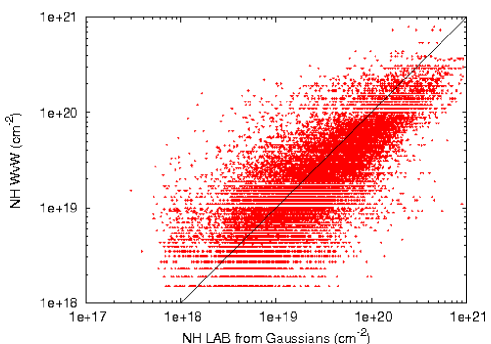
Figure 7: H i column densities from the WvW database in comparison with column densities determined from the LAB survey after Gaussian decomposition. All LAB profiles within HVC complexes according to WvW have been used. The solid line indicates the expected correlation.

3.2 Column densities from Gaussian components

We use the Gaussian components and display in Figs. 6 a comparison of LAB component column densities with those from the WvW catalog. The linear regression line shows $N_{H}({\rm LAB})/N_{H}({\rm WvW})=1.4$, consistent with the previous discussion. For Fig. 6 we use for each WvW position the nearest LAB position only. For Fig. 7 all of the LAB profiles next to each WvW position are considered, thus filling the 1.0^∘  (Hulsbosch & Wakker, 1988) or 2.0^∘  grid (Bajaja et al., 1985). If the HVC distribution were smooth, both plots would be identical. However, the large scatter in Fig. 7 degrades the expected correlation. A comparison of this kind is therefore highly problematic. In the same way it is quite a problem to compare LAB column density maps with maps generated from highly under-sampled observations on a 1.0^∘  or 2.0^∘  grid. This was noted already by Wakker (2004). Consistent maps were obtained only after smoothing the LDS to a 1.0^∘  beam and using a careful selected velocity range.

In 1991 the WvW database was the best all sky HVC catalog and formally it is still the most sensitive one. The one-sigma noise limit is 10 mK (Hulsbosch & Wakker, 1988) for the northern and 25 mK (Bajaja et al., 1985) for the southern part but possible systematic errors have not been taken into account, profile wings in particular may be affected. For the LAB survey (Kalberla et al., 2005) the side-lobe response was removed and residual errors are most probably below a level of 20 – 40 mK, an order of magnitude below typical errors for radio telescopes. Some compromises had to be made by Wakker & van Woerden (1991), notably on the velocity resolution and the sampling interval. Uncertainties in center velocities and velocity dispersions cause problems when selecting a velocity range. Moreover, the LAB survey shows significant real fluctuations. Under-sampling necessarily must cause inconsistencies. Hulsbosch & Wakker (1988) estimate that their catalog is 57% complete for clouds with a central peak brightness of 0.2 K. Smoothing the LAB to 1.0^∘  resolution helps a little when comparing with previous HVC maps (Wakker, 2004) but inconsistencies caused by an invalid interpolation of missing data in the WvW database due to a grid of 1^∘  or 2^∘  cannot be overcome.

4 Multi-component statistics

The previous sections have shown that the LAB survey has major advantages in its completeness on scales of 0.5^∘and in particular in its high velocity resolution, allowing an unbiased analysis for most of the observable HVC emission. Using a Gaussian decomposition (Haud, 2000), we found a large number of positions with a multi-component structure. In the following we shall focus on the properties of these multi-component features. We distinguish complexes according to the most recent classification by Wakker (2004) and find substantially different structures for individual complexes. This makes a discussion of individual complexes necessary. To keep this contribution comprehensive we shall focus on complex A, most of the other complexes are mentioned only briefly. On first reading individual subsections may be skipped.

4.1 Complex A

Complex A is one of the first discovered HVCs (Muller et al., 1963; Hulsbosch & Raimond, 1966). It’s distance is 8 to 10 kpc, the metallicity probably close to 0.1 times solar (van Woerden et al., 1999; Wakker, 2001; van Woerden & Wakker, 2004b). It’s velocity structure is complex, condensations tend to be associated with higher velocities (see e.g. Fig. 4 of Wakker, 2001).

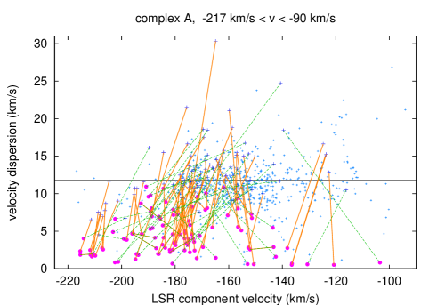
Figure 8: Distribution of the velocity dispersions of individual Gaussian components with respect to the observed LSR component velocities. The horizontal line indicates the mean dispersion $\sigma=11.8$ km s^-1. Crosses (blue) indicate primary, dots (magenta) secondary components. Solid lines (orange) connect components with $|v_{i}-v_{1}|<\sigma_{1}$, dotted lines (green) with $|v_{i}-v_{1}|<{\rm FWHM}_{1}$.

Fig. 8 shows the distribution of component velocity dispersions derived from the LAB survey with respect to the observed center velocities. The crosses indicate primary, the dots secondary components. At high velocities, $v\la-180$ km s^-1, we find predominantly narrow lines with dispersions lower than the average dispersion $\sigma=11.8$ km s^-1. For $v\ga-150$ km s^-1predominantly high velocity dispersions show up. To display the relations between primary and secondary components, observed at the same position, we have drawn a connection between these components. Solid lines were used in cases when the center velocity of the secondary component (index i) deviates from the primary component (index 1) by less than its dispersion, $|v_{i}-v_{1}|<\sigma_{1}$. For the hypothesis of a core moving within an envelope this indicates subsonic motions. Supersonic motions with $|v_{i}-v_{1}|<2.35\cdot\sigma_{1}$, corresponding to the FWHM line widths of the primary component, are indicated by dotted lines. We disregard larger Mach numbers $M=|v_{i}-v_{1}|/\sigma_{1}$, as Fig. 11 shows that these are unimportant.

Figure 9: Mean emission (solid line, red) and rms fluctuations (dashed line, green) from the LAB survey calculated for all positions where HVC emission was detected. The lower dotted line (blue) shows the mean emission from the secondary Gaussian components.

To demonstrate that secondary components unambiguously are related with small scale features we compiled for complex A three spectra, the mean H i emission of this complex for all LAB positions where HVC emission was detected, the corresponding rms deviation from the mean, and in addition the mean emission of the secondary components. The rms spectrum is most sensitive for small scale features, emission on scales $d\ga 0\hbox{$.\!\!^{\circ}$}5$ is filtered out (for discussion of the properties of rms spectra see e.g. Mebold et al., 1982). Fig. 9 shows that the emission from secondary HVC components is similar to the rms spectrum, except for an arbitrary scaling depending on the telescope beam width. The situation is different at intermediate velocities. Secondary IVC components, possibly associated with primary HVC components, are negligible.

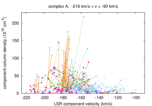
Figure 10: Distribution of component column densities with respect to the observed LSR component velocities. Crosses (blue) indicate primary, dots (magenta) secondary components. Solid lines (orange) connect components with $|v_{i}-v_{1}|<\sigma_{1}$, dotted lines (green) with $|v_{i}-v_{1}|<{\rm FWHM}_{1}$.

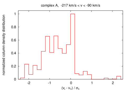
Figure 11: Column density weighted frequency distribution of $(v_{i}-v_{1})/\sigma_{1}$.

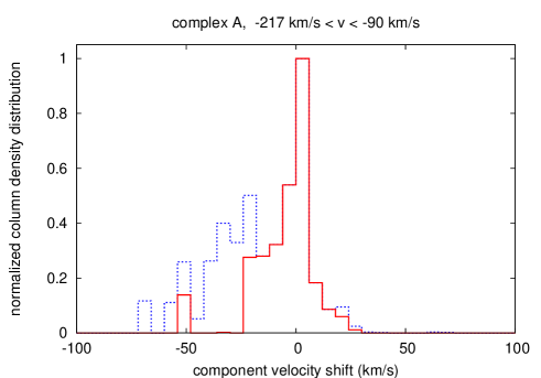
Figure 12: Column density distribution of secondary components with respect to their velocity shifts $v_{i}-v_{1}$. Solid lines are for subsonic components with $|v_{i}-v_{1}|<\sigma_{1}$, dotted lines for supersonic components up to Mach 2.35.

In Fig. 10 we display the HVC component column densities against their velocities. Symbols and lines have the same meaning as in Fig. 8. For $v\la-170$ km s^-1, a significant fraction of the HVC emission is contributed by secondary components. At $v\ga-150$ km s^-1  secondary components are insignificant but also the primary components have low column densities. Multi-component structure in complex A exists only at 13% of the positions but most of this is at high velocities.

Figs. 8 & 10 show a complicated dynamical network in 3-D, relating velocities, line widths and column densities between primary and secondary components. Some substructures appear to repeat. In particular, we find that many of the lines connecting primary and secondary components in Fig. 8 run parallel.

Fig. 11 shows the frequency distribution of $(v_{i}-v_{1})/\sigma_{1}$. A comparison between Fig. 4 and 5 demonstrates that the statistic depends on the weight. Rather then using number statistics we decided to weight for the rest of the paper components according to their column densities. To allow a better comparison we normalize in general the peak to 1. We find a bimodal situation. The narrow peak at $(v_{i}-v_{1})/\sigma_{1}\sim 0$ corresponds to cores with random motions and Mach numbers $M\la 0.5$. A broad distribution with $0.5\ga M\ga 1.5$ exists for cores at more negative velocities than the primary components. In Fig. 12 we plot the column density weighted distribution of the component velocity shifts $v_{i}-v_{1}$. The solid line represents components with $|v_{i}-v_{1}|<\sigma_{1}$, the dotted line is for the supersonic case. This histogram again shows a clear pattern. The peak around zero is due to the cores with the low Mach numbers. Another group of cores exist with velocity shifts up to $-50$ km s^-1, these are the clumps with larger Mach numbers.

The first moment of this distribution is at $v_{i}-v_{1}=-3.7$ km s^-1  for subsonic components and $v_{i}-v_{1}=-7.5$ km s^-1  for supersonic components (see Table 1). For a multi-phase medium in equilibrium one would expect a symmetrical distribution of component column densities around zero velocity shift. If a multi-component interpretation is valid for complex A we conclude that this HVC must be in a highly non-equilibrium state.

4.2 Complex C

Complex C is the second largest HVC complex and is at a distance $\ga 6$ kpc. The metallicity is $\sim 0.1-0.2$ solar (Wakker, 2004; Tripp et al., 2003). This complex has a broad distribution of H i gas between $-140\la V\la-110$ km s^-1  and some elongated filamentary structures at $v\la-140$ km s^-1. Multi-component structures are less prominent in comparison to complex A, see Table 1.

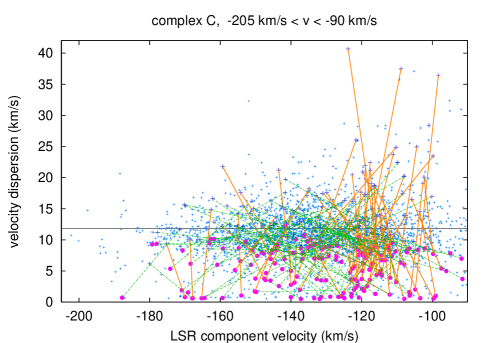
Figure 13: Same as Fig. 8 but for complex C.

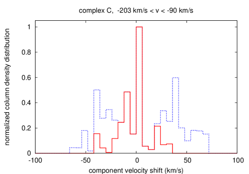
Figure 14: Column density distribution of secondary components with respect to their velocity shifts $v_{i}-v_{1}$. Solid lines are for subsonic components with $|v_{i}-v_{1}|<\sigma_{1}$, dotted lines for supersonic components up to Mach 2.35.

Fig. 13 shows the distribution of velocity dispersions and the relation between primary and secondary components. These appear to be distributed randomly, also we find no clear preferences in the column density distribution, much in contrast to Figs. 8 & 10. Velocity shifts between secondary and primary components are distributed in a nearly symmetric way, see Fig. 14.

4.3 Complex H

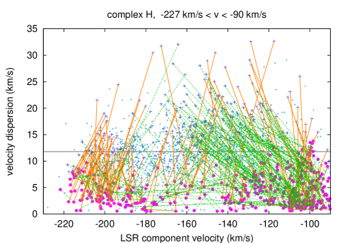
Figure 15: Same as Fig. 8 but for complex H.

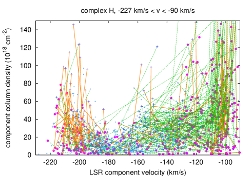
Figure 16: Same as Fig. 10 but for complex H.

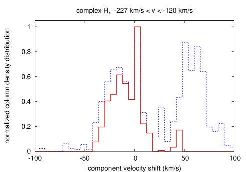
Figure 17: Column density distribution of secondary components with respect to their velocity shifts $v_{i}-v_{1}$. Solid lines are for subsonic components with $|v_{i}-v_{1}|<\sigma_{1}$, dotted lines for supersonic components up to Mach 2.35.

This complex, studied first by Hulsbosch (1975), lies in the plane of the Galactic disk and has an angular extent of $\sim 25\hbox{${}^{\circ}$}$. Blitz et al. (1999) proposed that it is located at a galacto-centric distance of $R\ga 40$ kpc. Lockman (2003) advocated $R=33\pm 9$ kpc. There are some different opinions which part of the emission should be related to the HVC or the disk. According to Wakker & van Woerden (1991) emission at $v<-80$ km s^-1  belongs to the HVC. Wakker (2004) considers only gas at $v<-90$ km s^-1. Blitz et al. (1999) pointed out that at least some of this gas belongs to the outer edge of the Milky Way disk.

First we consider the HVC with velocities $v<-90$ km s^-1. Fig. 15 shows the distribution of component velocity dispersions with respect to the observed center velocities. The velocities for most of the cores are systematically offset from their envelopes. Secondary components at $-220\la v\la-190$ km s^-1  are associated with envelopes at more positive velocities. The opposite happens for secondary components at $-140\la v$ km s^-1, these are associated with with envelopes at more negative velocities. Fig. 16 shows that cores with the most extreme velocities have the largest column densities. Cores at $-120\leq v$ km s^-1  have exceedingly large column densities, cut off in the plot. This part of the emission is most probably caused by the disk, for discussion see Sect. 6. We therefore exclude components at $v\leq-120$ km s^-1  for the further discussion, the entry in Table 1 is H(–120).

Most of the components with $v\la-190$ km s^-1  are subsonic. Plotting in Fig. 17 the component column density distribution for $v<-120$ km s^-1  with respect to velocity shifts $v_{i}-v_{1}$ we find a very broad distribution. The components group at several distinct velocity shifts $v_{i}-v_{1}$ , most prominent subsonically at $v_{i}-v_{1}\sim-20$ km s^-1  and supersonically at $v_{i}-v_{1}\sim 60$ km s^-1. These are mostly cores with $v\ga-150$ km s^-1.

Our interpretation of two components at different velocities in the same direction as physically related gas having subsonic or supersonic relative motions is not unique. As pointed out by the referee, the possibility exists that these components are well separated in distance. The bimodal nature of the shift suggests that we are looking at two objects, or at least at one object that is stretched and convoluted such that the sight-line crosses it twice.

Such an interpretation demands a spatial separation of primary and secondary components. A strict separation would be in conflict with the general finding that narrow lines are always associated with broad components, leading to the core-envelope hypothesis (Giovanelli et al., 1973). Cold components in the halo cannot exist on their own (Wolfire et al., 1995b). The assumption of an object which has two or more separate components along the line of sight demands that we need to take at least two broad components into account. These lines could blend to a single primary component but we expect in this case larger line-widths. Table 1 lists in column 9 the first moment of the column density weighted distribution of velocity dispersions. The entry for complex H, $\sigma_{NH}=12.0$ km s^-1  does not deviate significantly from the average $<\sigma_{NH}>=11.8$ km s^-1  for all Gaussians. Considering only those positions in complex H that have no associated secondary components, we obtain $\sigma_{NH}=11.0$ km s^-1, again identical with the value obtained for the whole sample. There are no indications that our interpretation is affected by a complicated spatial substructure. We generalize this result for most of the complexes. MS, C, WA, and WC may be affected for some of the sight-lines. The interface region close to the Magellanic System most probably has a complicated spatial structure, we consider this in Sect. 4.5.

4.4 Complex M

Danly et al. (1993) determined a distance to complex M of $1.5\la z\la 4.4$ kpc. Wakker (2001) cites a metallicity of $\sim 0.8$ solar. In complex M the average velocity dispersion of the Gaussian components is low, $\sigma\sim 10.3$ km s^-1. We find only 19 positions with multi-component structure. The secondary components tend to be associated with large column densities (Fig. 18). The velocities of most of the cores are shifted to larger velocities.

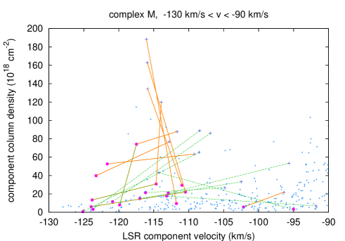
Figure 18: Same as Fig. 10 but for complex M.

4.5 Complex MS

The Magellanic Stream can be explained as a tidal tail of the Small Magellanic Cloud (Gardiner & Noguchi, 1996). According to (Wakker, 2004) it extends over 120^∘  and the LSR velocities range from $-440$ to $+412$ km s^-1. Following Brüns et al. (2005, Figs. 3,4) we restricted this range significantly. We excluded any emission possibly related to the LMC or the SMC, also to the interface region by selecting a latitude limit $b<-61\hbox{${}^{\circ}$}$. In addition we splitted this huge complex into two parts with positive and negative LSR velocities. In both cases we deviate from the condition that Gaussian components should have $|v|>90$ km s^-1. We allow $|v|>50$ km s^-1since we found no problems caused by confusion with the local gas. The positive velocity part, MS+, contains 27% of the gas in secondary components (Fig. 19), while the negative velocity part, MS–, has only 10% of the gas in cores (Fig. 20). MS+ shows some scatter in the velocity shifts but no trend on average, some of the clumps have large column densities. The properties of secondary components in MS– are quite different. The velocities of the secondary components are significantly higher, on average shifted by $-9$ km s^-1  with respect to the primaries.

In Table 1 we included for comparison the entry MS+W, according to the definition by Wakker (2004), unrestricted with respect to the interface region. Also in this case a significant fraction of the HVC emission is found in secondary components. Excluding the interface region has cut off 20^∘  of the stream and restricted the velocities to $v\la 206$ km s^-1  but did not affect the statistical properties of its Gaussian components significantly.

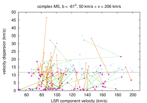
Figure 19: Same as Fig. 8 but for complex M.

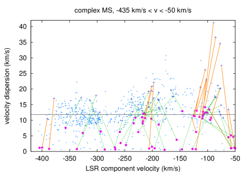
Figure 20: Same as Fig. 8 but for complex M.

4.6 Complex EP

This is the leading arm of the Magellanic Stream. According to Wakker (2004) the LSR velocities of this HVC are in the range 103 to 354 km s^-1. We find emission from the disk up to LSR velocities of 170 km s^-1  and restrict therefore the velocity range accordingly. The HVC emission lines are very narrow at all velocities (Fig. 21). The first moment of the column density weighted distribution of the velocity dispersions is 11.5 km s^-1. There are no obvious shifts between the center velocities of secondary and primary components.

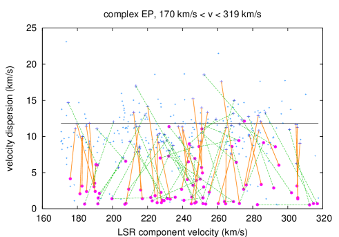
Figure 21: Same as Fig. 8 but for complex EP.

4.7 Complex ACHV & ACVHV

First observations of the anti-center HVCs have been published by Hulsbosch (1968), a more detailed discussion is given by Wakker & van Woerden (1991). Neither distances nor metallicities are known. 4% of the observed positions show a multi-component structure. The lines are in general broad in complex ACHV, even for most of the secondary components. Fig. 22 shows the distribution of component velocity dispersions. The velocity shifts show a broad scatter, some of the components tend to have shifts of $\sim-30$ km s^-1.

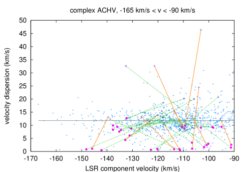
Figure 22: Same as Fig. 8 but for complex ACHV.

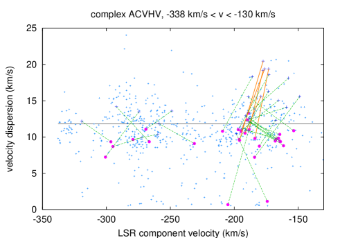
Figure 23: Same as Fig. 8 but for complex ACVHV.

Fig. 23 shows a very different distribution of component column densities for comples ACVHV. Secondary components are not very frequent. A grouping at velocities $-200\la v\la-160$ km s^-1  for HVC ACI and $-300\la v\la-250$ km s^-1  for HVC 168–43–280 is obvious.

4.8 Complex WB

Thom et al. (2006) report a distance determination in direction to this complex and suggest a distance $7.7<d<8.8$ kpc. Hence WB would be located at $z\sim 7$ kpc and $R\sim 12$ kpc. As pointed out by the referee, it may be questioned whether this limit applies for complex WB. Thom et al. (2006) find an upper limit to a small HVC (cloud 35) that was not included as part of this complex by WvW. The ”real” complex WB is a mostly-connected cloud at somewhat lower latitudes. There are many tiny positive-velocity HVCs at somewhat higher latitudes in this part of the sky, which may be part of the same complex.

Most of the subsonic secondary components for complex WB (solid lines in Fig. 24) are shifted to higher velocities. Some of the supersonic cores behave in the opposite way (dashed lines).

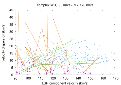
Figure 24: Same as Fig. 8 but for complex WB.

4.9 Complex WD

Wakker (2004) lists this HVC with velocities $94<v<278$ km s^-1. We find very little gas at $v\ga 170$ km s^-1. Secondary components are shifted predominantly to higher velocities (Fig. 25).

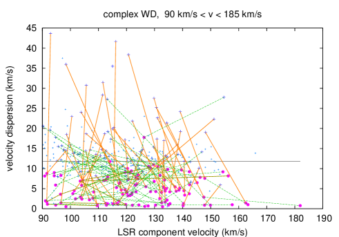
Figure 25: Same as Fig. 8 but for complex WD.

4.10 Complex WE

Sembach et al. (1991, 1995) determined an upper distance limit of $\sim 12.8$ kpc. Similar to Complex WD we find no H i emission at $v\ga 136$ km s^-1. From (Wakker, 2004) we expect emission up to $v=195$ km s^-1, but apparently this part of the HVC emission is weak. There are no systematic shifts in velocities between primary and secondary components. Fig 26 looks rather chaotic.

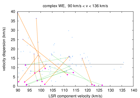
Figure 26: Same as Fig. 8 but for complex WE.

4.11 Complex R

This HVC was first studied by Kepner (1970), who suggested that it might be due to gas raining down to the disk. At velocities $v\ga-120$ km s^-1  there is overlap with disk emission. Narrow components in this velocity range may indicate interaction with the disk (Fig. 27).

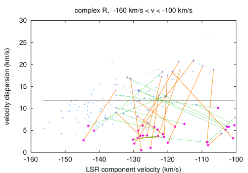
Figure 27: Same as Fig. 8 but for complex R.

4.12 Complex G

This gas has a lower distance limit of 1.3 kpc (Wakker, 2001). At velocities $v\la-160$ km s^-1  we find no secondary components (Fig. 28).

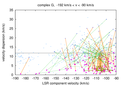
Figure 28: Same as Fig. 8 but for complex G.

4.13 Disk material

Complex OA is usually interpreted as part of the outer arm, reaching intermediate latitudes (Habing, 1966; Haud, 1992). From the rotation curve we estimate a distance of 15 - 20 kpc for gas at velocities of $-130$ km s^-1. Secondary components are found at 42% of all positions, twice the average for all HVCs, but these components contain only 24% of the observed column densities (see Table 1). This gas has most probably properties similar to the H i in the disk. For such a multi-phase medium one would expect random internal motions. Indeed, we find no preferences, grouping or other relations between primary and secondary components. Fig. 29 reflects this situation. The distribution of component velocity shifts is nearly symmetric.

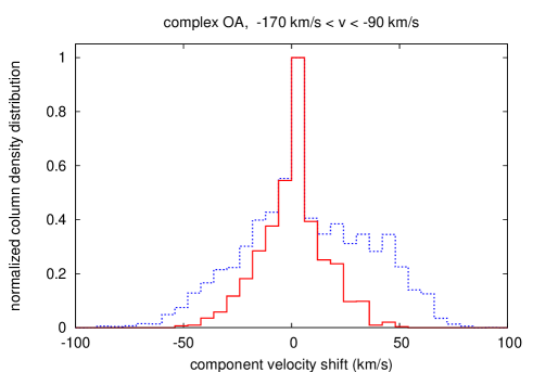
Figure 29: Column density distribution of secondary components with respect to their velocity shifts $v_{i}-v_{1}$. Solid lines are for subsonic components with $|v_{i}-v_{1}|<\sigma_{1}$, dotted lines for supersonic components up to Mach 2.35.

Similar to complex OA the number of positions in complex GCP with multi-component structure is large, however the associated column density is less prominent. The relations between primary and secondary components appear to be purely statistical (Fig. 30). Some similarities to complex OA may be a hint that this complex is closely associated with the disk.

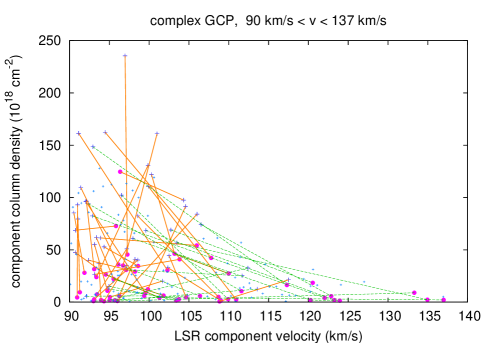
Figure 30: Same as Fig. 10 but for complex GCP.

4.14 Non-detections or questionable cases

The extreme negative velocity clouds in complex EN contain only a few multi-component detections (Fig. 31). Wakker (2004) classifies these clouds with velocities $-465<v<-132$ km s^-1. For $v\ga-220$ km s^-1  we found significant contributions from Galactic plane gas. We therefore excluded this range.

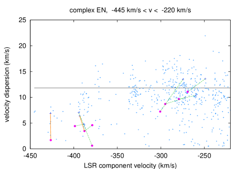
Figure 31: Same as Fig. 8 but for complex EN.

Complexes WA and WC contain very little gas in secondary components. Most of the narrow lines have very low column densities and may therefore be spurious. WA and WC have each only two significant secondary components. Remarkable is, however, that most of the secondary components in complex WA, if real, are very cold and shifted by 36 km s^-1  relative to the LSR velocity of the primary components (Fig. 32). WC is different, the components are also cold but it shows a broad scatter of the velocity shifts.

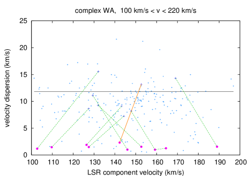
Figure 32: Same as Fig. 8 but for complex WA.

In three complexes we found only one position with multi-component structure, L, GCN, and D. In complex P we have 5 detections, but 3 with very low column densities. The complexes discussed in this section have less than 3% of the gas in cores.

5 HVC - IVC interaction

Observational indications for interactions of HVCs with the Galactic disk have been claimed for several HVC complexes, we refer to the most recent review by Brüns & Mebold (2004). HVCs approaching the disk are expected to be decelerated by ram pressure (Benjamin & Danly, 1997). In turn, shocks may lead to fragmentation and phase transitions. Head-tail structures (Brüns et al., 2000) may develop and velocity-bridges (Pietz et al., 1996) may connect individual H i HVC fragments in the velocity-position space. Strong interaction may lead to collisional ionization, observable in H $\alpha$  (Weiner & Williams, 1996) or O vi absorption (Sembach et al., 2003). X-ray enhancements (Kerp et al., 1996) or even $\gamma$-ray emission (Blom et al., 1997) may be caused.

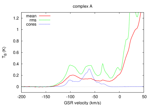
Figure 33: Mean emission (solid line, red) and rms fluctuations (dashed line, green) from the LAB survey calculated for all positions where HVC emission was detected. The lower dotted line (blue) shows the mean emission from the secondary Gaussian components. The data are the same as displayed in Fig. 9 but here we use GSR velocities.

Here we intend to discuss whether from the Gaussian decomposition any evidence for an interaction between HVCs and IVCs can be found. The spatial distribution of HVC complexes overlaps partly with IVC features, see e.g. the reviews by Wakker (2004) or (Albert & Danly, 2004). The question arises whether the positional agreement between both components is accidental or whether there might be some evidence for an interaction.

5.1 The HVC rest frame: LSR, GSR, LGSR or deviation velocity?

Up to now we avoided any interpretation about origin and distances of HVCs. All parameters have been described in the Local Standard of Rest (LSR) frame. Observations in this frame are corrected for the basic solar motion and tied locally to a rotating Galactic disk. If HVCs are associated with the Milky Way but not co-rotating with the disk, the Galactic Standard of Rest (GSR) would be more appropriate for a description. It is also possible that HVCs are building blocks from which the Local Group was assembled (Blitz et al., 1999), in this case the Local Group Standard of Rest (LGSR) would be the best choice. Equations for a conversion between different systems are given by de Heij et al. (2002c). Last, not least, HVCs are characterized sometimes by their deviation velocities (Wakker, 1991). This measure is not tied to an interpretation but allows to judge how significant HVCs are separated from the Galactic disk emission. A display of the HVC sky in deviation velocities as well as GSR velocities is given by Wakker (2004).

Fig. 9 shows in the LSR rest frame the mean emission and emission fluctuations derived for all positions of complex A that show HVC emission. In addition we plot the mean emission for the cores only. Most of the gas, in particular the emission from the cores, is clearly separated from the disk and the IVC emission at $v\sim-50$ km s^-1. The picture changes significantly if we use GSR velocities (Fig. 33). The HVC separation from the disk emission is less obvious. Projection effects cause the core emission to be much closer to the mean disk emission at $v\ga 0$ km s^-1. The prominent IVC feature is washed out completely in velocity. A projection of complex A into the LGSR system shows a similar picture, shifted approximately by 40 km s^-1, and we conclude that complex A, considered as a single coherent cloud, is distinguished best from the local gas and the IVC emission in the LSR system. IVCs, anyway, are best described in the LSR system.

There is no space to display other examples in the GSR or LGSR frame but it is clear from this example that the LSR frame is appropriate to discuss the question whether some of the HVCs might be interacting with the disk. In this frame the HVC velocities differ typically by several tens of km s^-1  from IVCs and the disk emission. An interaction between HVC and disk gas necessarily would lead to strong shocks and we would expect to find cold, dense H i clouds as tracers of such an interaction. Secondary components at low velocities, associated with primary components at large velocities, may indicate such shocks. The search algorithm used in Sect. 4 was biased since we rejected any Gaussian component with velocities below the pre-defined lower velocity limit (see column 4 of Table 1, typically $|v|>90$ km s^-1).

To find features indicating a possible HVC/IVC interaction we extend our search algorithm. We allow primary components at high velocities to be associated with secondary components at low velocities. The mere existence of such pairs of Gaussians is not a sufficient proof for an interaction. Such components may show up accidentally along the line of sight. However, finding numerous cases would be in favor for an interaction. The interaction hypothesis can be rejected if our search fails to find such component pairs. We discuss the easy case first.

5.2 No indications for HVC/IVC interaction in complex A, MS, ACVHV, EN, WA, & P

Fig. 9 shows that along the line of sight to Complex A also a significant contribution at intermediate velocities is observed. Both, the mean emission profile as well as the rms deviation from the mean, peak at $v\sim-55$ km s^-1. However, from the Gaussian decomposition, there is no significant evidence for secondary components at velocities $v\ga-90$ km s^-1. Extending our search algorithm does not disclose new components and we conclude that there are no indications for IVC cores associated with primary HVC components.

Our conclusion that there is no HVC/IVC interaction in direction to complex A is consistent with previous distance determinations. Complex A is at a z height of 5 to 7 kpc (van Woerden et al., 1999; van Woerden & Wakker, 2004b), far above the IVC gas layer with typical upper limits of $1\la d\la 4$ kpc (Albert & Danly, 2004). No interaction is expected.

Similar to complex A we find no indications for an HVC/IVC interaction for the Magellanic stream and complexes ACVHV, EN, WA, and P. We list in Table 1 the fraction $f_{NIV}$ of the column density observed at intermediate velocities, outside the HVC velocity range listed in column 4 of Table 1. For all of these complexes $f_{NIV}<0.01$.

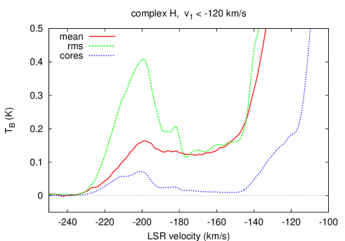
Figure 34: Mean emission (solid line, red) and rms fluctuations (dashed line, green) from the LAB survey calculated for all positions where HVC emission was detected. The lower dotted line (blue) shows the mean emission from the secondary Gaussian components.

5.3 Complex H

Figs 15 to 17 in Sect. 4.3 gave evidence for a bimodal distribution of the secondary components associated with primary components in complex H. Cores at high velocities move typically 20 to 30 km s^-1faster than the envelopes while cores at low velocities are slow by 50 to 70 km s^-1. Fast cores move predominantly subsonically, slow cores are mostly supersonically. Fig. 34 shows the same bimodal distribution for the mean emission (solid line) and its rms fluctuations (dashed). A broad minimum exists between $-180\la v\la-150$ km s^-1, a “velocity bridge” according to (Pietz et al., 1996), indicating a possible interaction between gas at high and low velocities. The mean emission from the cores (dotted line in Fig. 34) has a similar velocity bridge between $-180\la v\la-150$ km s^-1and a strong increase for $v\ga-150$ km s^-1. There is a marked contrast to complex A (Fig. 9) and the complexes discussed in the previous section. We find a large number of narrow lines for $v\ga-150$ km s^-1, exclude therefore chance coincidences and interpret the secondary components as a population of cold, shocked clumps, most probably caused by an interaction between HVC and disk gas. More than 30% of the total observed column density in direction to complex H is at velocities $v>-120$ km s^-1.

A part of complex H was observed recently by Lockman (2003) with the GBT. Lockman suggested that this object could be a satellite of the Milky Way, interacting with the Galactic disk. He determined a distance of $d\sim 27$ kpc, or $R\sim 33\pm 9$ kpc. The GBT observations gave also evidence for a multi-phase medium. A group of condensations at galactic coordinates $l\sim 131\hbox{${}^{\circ}$}$, $b\sim 1\hbox{${}^{\circ}$}$ is particularly interesting since its small scale structure at scales of 4^′  is known (Wakker & Schwarz, 1991) and, most important, a spin temperature of $T\sim 50$ K (Wakker et al., 1991) was measured. This allows for an accurate determination of an internal pressure $P/k\sim 100$ cm^-3K for the cores at a LSR velocity $v\sim-200$ km s^-1. Moreover, a similar pressure was determined with the GBT for the surrounding envelope, a convincing argument for a multi-phase medium in pressure equilibrium (Lockman, 2003).

How about the Milky Way disk? Using a model of the Galactic H i distribution (Kalberla, 2003), we expect an average pressure of $P/k\sim 100$ cm^-3K for gas in the disk at a LSR velocity of $v\sim-130$ km s^-1  and a distance $d\sim 26$ kpc, or $R\sim 32$ kpc, just at the position of complex H as estimated by Lockman (2003). Using alternatively a rotation curve according to Brand & Blitz (1993) would result in a slightly different LSR velocity of $v\sim-124$ km s^-1  and a 30% larger pressure. An inspection of the LAB survey gives a clear evidence for continuous H i emission at such velocities as expected for the outskirts of the disk, see also Blitz et al. (Fig. 3 of 1999) or Lockman (Fig. 3 of 2003). Most of the emission at LSR velocities of $-120\la v\la-90$ km s^-1  originates from the Galactic disk. Emission from the clumps at $-150\la v\la-120$ km s^-1(Fig. 34) is most probably caused by a HVC/IVC interaction.

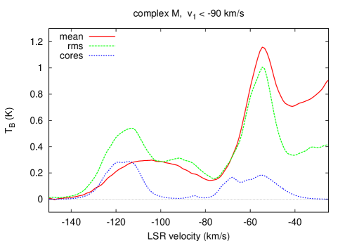
Figure 35: Mean emission (solid line,red ) and rms fluctuations (dashed line, green) from the LAB survey calculated for all positions where HVC emission was detected. The lower dotted line (blue) shows the mean emission from the secondary Gaussian components.

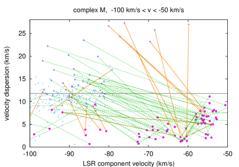
Figure 36: Same as Fig. 8 but for complex M.

5.4 Complex M

We apply our search algorithm for IVC clumps also to complex M. We find again a bimodal distribution of the core velocities. Clumps at $-80\la v\la-40$ km s^-1(Fig. 35) may be associated with HVC envelopes at higher velocities. Fig. 36 shows the relation between cores and envelopes in more detail. We find a highly non-random distribution, most of the lines connecting cores and envelopes run parallel. The similarity with the low velocity part of complex H (Fig. 15) is striking.

Distance and metallicity of complex M were discussed recently by van Woerden & Wakker (2004b). The upper limit of its distance is $z\la 3.5$kpc. The high metallicity (0.8 solar) suggests an association with the Intermediate-Velocity Arch, which lies at a distance of 0.8 to 1.8 kpc. The association between high velocity envelopes and low velocity cores provides additional evidence for a possible interaction.

5.5 Complex C

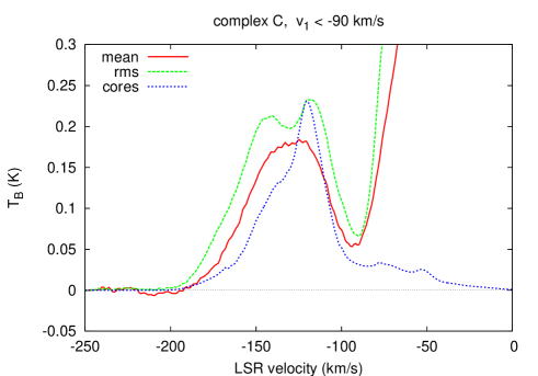
Figure 37: Mean emission (solid line, red) and rms fluctuations (dashed line, green) from the LAB survey calculated for all positions where HVC emission was detected. The lower dotted line (blue) shows the mean emission from the secondary Gaussian components.

Also complex C is of particular interest. In Fig. 37 we display profiles for the mean emission, its rms fluctuations and the emission due to secondary components. The emission from the cores peaks at $v\sim-120$ km s^-1and has an extended tail to lower velocities. A number of secondary components appear to be related to primary components at larger velocities, however the total amount of gas in cores at intermediate velocities is lower than in the cases discussed in Sect. 5.3 & 5.4. Complex C is the second largest after complex OA but apparently only a fraction of it shows signs of interaction.

Using the LDS, Pietz et al. (1996) detected H i velocity bridges in complex C connecting HVC gas with intermediate velocities. Effelsberg observations with better resolution confirmed the reality of these features. Using the ROSAT all-sky survey, Kerp et al. (1996) found soft X-ray enhancements in the same directions and took this as an indication for an impact of HVCs onto the Galactic disk. (Brüns et al., 2000) found head-tail structures and concluded that these cometary features are caused by interaction. Wakker (2004) argues against a possible connection between complex C and intermediate velocity clouds (IVC) in the intermediate velocity Arch IV (Kuntz & Danly, 1996). Abundances and their variations in direction to complex C may provide clues for the origin of this HVC gas. Wakker et al. (1999); Richter et al. (2001a); Tripp et al. (2003) found evidence for the infall of low-metallicity gas onto the Milky Way, we refer to the most recent discussion by van Woerden & Wakker (2004b, Sect. 6.1).

5.6 Complex WB, WD, WE, WC, R, G, GCP, & OA

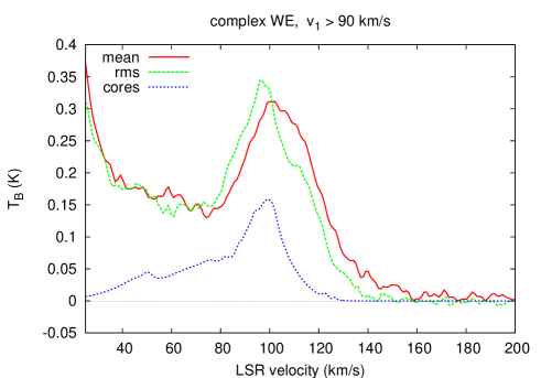
Figure 38: Mean emission (solid line, red) and rms fluctuations (dashed line, green) from the LAB survey calculated for all positions where HVC emission was detected. The lower dotted line (blue) shows the mean emission from the secondary Gaussian components.

In all cases we find low velocity wings for the mean emission of the secondary components. The mean emission profiles in direction to these HVCs, similar the rms deviations, have extended wings toward zero velocities. The wings for the mean emission are caused by differential Galactic rotation. In Sect. 5.2 we found no indications that secondary components may be seriously affected due to blending with foreground or background sources. For the complexes discussed here the lines of sight are more complex and we cannot exclude that a significant part of the secondary components at intermediate velocities may be spurious.

Complex WE is of particular interest since an upper distance limit of $d\la 12.8$ kpc ($z\la 3.2$kpc) is known (Sembach et al., 1991, 1995; Wakker, 2001). Fig. 38 displays the derived spectra for mean emission, rms deviations, and emission from cores.

6 Discussion

We have decomposed the LAB survey database into Gaussian components. All HVC complexes have been searched for indications of a multi-phase medium. We obtained clear indications for two H i phases, broad lines with a typical velocity dispersion of 12 km s^-1  dominate. Narrow lines with typical dispersion of 3 km s^-1  are found predominantly in regions with high HVC column densities. In many cases the secondary components have systematic velocity shifts relative to the broad primary components but we observe also a large scatter. The properties of the HVC cores, listed so far, are known since Cram & Giovanelli (1976). However, our investigations provide a much larger sample. All of the major HVC complexes show indications for a multi-component structure. Depending on the individual complexes up to 38%, on average 24%, of the positions with HVC emission have multiple HVC Gaussian components. These are predominantly positions with large column densities. Up to 27%, on average 20%, of the observed HVC flux originates from cold cores. Our analysis covers large complexes only. In the case of compact HVCs (CHVCs) de Heij et al. (2002a) find 4 – 16% in the cold phase.

Clear indications for a multi-phase structure in complex EN, WA, WC, P, L, GCN, and D are missing. All-together these cover about 6% of of all sky positions where we find HVC emission. The question arises whether these complexes might be special or whether the LAB data simply might not be adequate for these complexes. Giovanelli et al. (1973) have pointed out that cores are small scale features, barely resolved with a beam of 0.5^∘. The LAB has a similar beam size and we need to take into account that this fact causes some restrictions.

The distances to most of the HVCs are unknown but complex H, MS, and EP are important exceptions. Cold cores do exist at a distance of $\sim 50$ kpc. This implies that the cores must have typical dimensions of a few hundred pc, otherwise beam dilution would heavily degrade the signal. High resolution observations are needed to resolve the cores and in particular to verify whether there is an interaction between gas at high and intermediate velocities (Pietz et al., 1996; Brüns et al., 2000; Lockman, 2003).

Wakker & Schwarz (1991) have demonstrated how important high-resolution interferometric observations are for a detection of cores. They used the WSRT to map two clouds. Six compact isolated HVCs have been mapped by Braun & Burton (2000) and six more by de Heij et al. (2002a). Burton et al. (2001), using the Arecibo telescope, confirm that essentially all CHVCs have a core-halo structure, for discussion see Sect. 5 of Burton et al. (2004). Velocity dispersions derived for CHVCs are somewhat smaller, but taking beam smearing into account, in any case consistent with values derived by us. We conclude that most probably our results can be generalized in the sense that all HVCs have a multi-phase structure. The probability to detect cold cores would then depend merely on telescope sensitivity and resolution.

The conditions for a multi-phase medium in the Galactic disk and the halo have been discussed by Wolfire et al. (1995a, b). A stable two-phase H i gas can exist over a range of heights but only within a narrow range of pressures at each height. It was shown that a hot ($T\sim 1-2\cdot 10^{6}$ K) halo can provide the necessary pressure. Observations of a multi-phase medium can, in principle, constrain distances of HVCs, provided their metallicity and dust-to-gas ratio is known.

For a few complexes a multi-component structure is rather unexpected. The first is the part of the Magellanic stream at LSR velocities $50\la v\la 362$ km s^-1($50\la v\la 201$ km s^-1without the interface region). This gas is approximately at a distance of 50 kpc. Wolfire et al. (1995b) predicted that a multi-phase medium associated with the Magellanic stream should exist only at distances $z\la 20$ kpc above the disk. Fig. 19, however, shows a well defined two-component structure. The number of positions with such a structure as well as the associated column densities are even larger than the average, see Table 1. Cores with narrow lines were found also in the leading arm (complex EP). This HVC is usually estimated to be at a similar distance, a two-phase H i medium is therefore also unexpected. High resolution Parkes observations of the Magellanic stream and the leading arm confirm a multi-component structure for the leading arm (Brüns et al., 2005). Molecular hydrogen, detected by Richter et al. (2001b) and Sembach et al. (2001), is another indicator for a multi-phase structure.

The trailing part of the Magellanic stream at negative LSR velocities differs significantly. It was found to have less secondary components. This may indicate a lower confining halo gas pressure and/or a larger distance for this part, as expected for a tidal origin (Gardiner & Noguchi, 1996).

Comparing the observational evidence for a multi-phase medium with model predictions (Wolfire et al., 1995b), we find it difficult to explain such a medium, at least for an assumed temperature of $T\sim 10^{6}$ K. Using the model of the gas distribution proposed by Kalberla (2003) we estimate a pressure of $P/k=nT\sim 20-40\leavevmode\nobreak\ {\rm cm}^{-3}\leavevmode\nobreak\ {\rm K}$ for complex MS+ and EP, probably still too low to explain the existence of a multi-phase medium. It appears necessary to reconsider the conditions that allow a multi-phase H i medium at such a distance in more detail.

The most recent analysis on the temperature of the hot halo is by Pradas et al. (2006) who have correlated the LAB survey with the ROSAT all-sky survey. Using simultaneously all ROSAT energy bands they were able to fit the observations with two plasma components, the first originating from the local hot bubble with a temperature of $T=10^{5.9}$ K and the second from the halo with a temperature of $T=10^{6.15}$ K. This increases estimates for a lower limit of the halo pressure by a factor of two. Additional arguments for a high pressure in the halo have been given by Weiner & Williams (1996); Sembach et al. (2003); Fox et al. (2004, 2005). Halo densities of up to $10^{-4}$ cm^-3 are proposed close to the Magellanic stream and the leading arm. Such densities would increase the halo pressure up to a factor 10. Interestingly, $10^{-4}$ cm^-3 is also the density required to explain compression fronts and head-tail shaped features in HVCs (Quilis & Moore, 2001), that have been found by Brüns et al. (2000, 2001) in almost all of the HVC complexes.

Another unexpected case is complex H, lying in the plane of the Galactic disk. Lockman (2003) located this HVC at a distance $R\sim 33$ kpc from the center and found evidence for a multi-phase medium at a pressure of $P/k=nT\sim 100\leavevmode\nobreak\ {\rm cm}^{-3}{\rm K}$. In Sect. 5 we argued that the gas in the disk has a similar pressure. Also the disk shows a two-component structure and there are indications for an interaction between disk and HVC. According to Wolfire et al. (2003) a multi-phase medium may exist in the Milky Way at distances $3\la R\la 18$ kpc. It appears necessary to consider the question whether the upper distance limit needs to be revised. Our results indicate that current models underestimate the halo gas pressure.

The situation may be different in compact high velocity clouds (CHVCs). Sternberg et al. (2002) discussed the conditions for a multi-phase structure in such objects. CHVCs have not been included in our sample since the spatial resolution of the LAB survey is not appropriate for these objects.

HVC complexes show some similarities in their internal velocity structure. To characterize this we derived velocity shifts $v_{i}-v_{1}$ between cores and envelopes and characterized the average internal motions by the first and second moments of the column density weighted distribution of the velocity shifts. Most of the HVCs have internal turbulent motions with Mach numbers between 1 and 2. These internal motions within HVCs should be compared with the properties of the disk gas. Heiles & Troland (2003), from an analysis of Arecibo absorption lines, find that cold clumps in the disk move only slightly supersonic within the surrounding warm neutral medium. Cores within HVCs are apparently faster. Our analysis may be biased. We excluded Gaussian components with velocity shifts $v_{i}-v_{1}>2.35\sigma_{1}$. Some HVC cores with very large turbulent motions may have been rejected, the derived typical Mach number $M\sim 1.5$ is therefore a lower limit only.

Next we consider the column density weighted standard deviation of Gaussian component center velocities. Heiles & Troland (2003) find $\sigma_{WNM}\sim 11$ km s^-1  for the WNM and $\sigma_{CNM}\sim 7$ km s^-1  for the CNM in the disk, consistent with previous results (e.g. Mebold et al., 1982). The situation for the relative motion of cold cores in HVCs is very different. We determine a column density weighted velocity dispersion $\sigma\sim 20$ km s^-1  for velocities $v_{core}-v_{envelope}$ (last column in Table 1). Davies et al. (1976) have noted this effect first in complex A IV and described it as feature-to-feature velocity differences. HVC cores typically move three times faster than cold clumps in the disk, only complex M has $\sigma\sim 10$ km s^-1  and deviates significantly in this respect.

The envelopes share the highly turbulent state of the clumps. Blitz et al. (1999, their Table 2) determined the variation of HVC line centroids from one position to the other and derived $\Delta v=30$ km s^-1. This, once more, is three times the value derived by Heiles & Troland (2003) for the warm H i phase in the disk. Individual HVC components represent a highly turbulent gas phase. The turbulent energy density of individual clumps of HVC gas is an order of magnitude larger than that of comparable clumps in the Galactic disk.

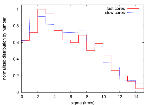
Figure 39: Normalized frequency distribution of secondary component line widths. The solid line represents secondary components moving faster than the primary components, $|v_{i}|>|v_{1}|$, the dotted line those moving slower. Selected were all complexes except OA and all secondary components with velocities $|v|>90$ km s^-1.

Despite having large internal motions, HVCs tend also to have ordered internal motions relative to their envelopes. This can be seen best for complex H in Fig. 15 for $v\ga-160$ km s^-1. Table 1 shows that cores are typically 5 km s^-1  faster than the associated envelopes. This is in good agreement with Cram & Giovanelli (1976) who derived an average velocity difference of 4.5 km s^-1. Contrary, we found also a population of clumps that move slower than the associated primary components, best seen in Fig. 15 for $v\la-160$ km s^-1. Is there a systematic difference between fast and slow moving cores?

We calculated the distribution of velocity dispersions for the secondary components of all HVC complexes, except complex OA. The outer arm was excluded since most probably this complex belongs to the disk population. We distinguish between fast moving HVC cores ($|v_{i}|>|v_{1}|$) and slow moving HVC cores ($|v_{i}|<|v_{1}|$) both with $|v|>90$ km s^-1. Fig. 39 shows that components with $\sigma\sim 2$ km s^-1  are most frequent but there is also a broad wing due to components with larger dispersions. Both distributions are very similar, systematical deviation probably barely significant. Internal motions of cold cores within the envelopes of HVC complexes are on average well balanced.

An inspection of Table 1 gives the impression that those HVC complexes that have the lowest observed gas fraction in cores $f_{n}$ (by number) or $f_{N}$ (by column density) tend to have the most negative velocities. We therefore calculated the number of positions with secondary components relative to the total number of components and the sum of column density in secondary components relative to the total column density as a function of the component velocity. In both cases we find a clear trend that the gas fraction in cores increases systematically towards the positive velocities. This remains valid also after repeating the analysis in the GSR or LGSR system.

7 Summary and conclusion

Using the LAB survey we derived the main observational parameters for most of the well known HVC complexes. Performing a consistency check with the WvW catalog (Wakker & van Woerden, 1991) we found a good agreement for the peak temperatures. Center velocities of the WvW catalog turned out to be accurate to 8 km s^-1but large discrepancies are found for the WvW velocity dispersions. These are not an appropriate description of the line widths and systematically biased. On average the WvW line widths and also the derived column densities need to be scaled upward by a factor of 1.4.

A systematic bias in the WvW catalog has some important consequences. Most of the derived global properties for HVCs, like masses of HVC complexes, also the net inflow of H i HVC gas come from this catalog (Wakker & van Woerden, 1997). These numbers need to be revised upwards by 40%. Pressures, derived for the diffuse part of the HVCs (e.g. Wakker & Schwarz, 1991) depend on $\sigma^{2}$, hence need to be revised by a factor of $\sim 2$. Timescales estimated for a free expansion of HVCs (Wakker & van Woerden, 1997) decrease accordingly.

Our Gaussian decomposition of the LAB survey led to the result, that most of the HVC complexes have a multi-phase medium. Cores with narrow lines ($\sigma\ga 2$ km s^-1) are embedded in envelopes with broad lines ($\sigma\sim 12$ km s^-1). According to Wolfire et al. (1995b) this may be taken as an indication that the HVCs are on average in pressure equilibrium with a surrounding hot halo. We find a multi-phase structure even at large distances, for complex H at $R\sim 33$ kpc, for the Magellanic stream, and the leading arm at distances $D\sim 50$ kpc. Current models do not support a sufficiently large halo pressure at such distances and need to be re-discussed. The fact that more than 90% of the HVC gas in complexes, excluding CHVCs, has a multi-component structure strengthens arguments that these clouds are associated with the Milky Way.

We characterize the motion of HVC cores within the associated envelopes by defining relative internal motions $v_{core}-v_{envelope}$ and Mach numbers $M=|(v_{core}-v_{envelope})|/\sigma_{envelope}$. On average we find Mach 1.5. Despite the fact that some HVC cores show ordered motions there are on average no preferences for the direction of the internal motions. The case $v_{core}-v_{envelope}>0$ is as frequent as $v_{core}-v_{envelope}<0$. The center velocities for the cores within a HVC complex show a typical dispersion of 20 km s^-1. The relative motion of HVC clumps is three times larger than the value derived for the motion of comparable clumps of CNM within the Galactic disk. HVCs are highly turbulent. The internal turbulent energy density of individual clumps of HVC gas exceeds that of the disk gas by an order of magnitude.

Table 1: Properties of HVC complexes. The columns are: name, longitude, latitude, velocity range, number of positions observed $n_{pos}$ , fraction of positions with cores: $f_{n}$, fraction of column density in cores relative to the total column density: $f_{N}$, fraction of column density in cores at intermediat velocities: $f_{NIV}$, first moment of the column density weighted distribution of velocity dispersions: $<\sigma_{NH}>$, first moment of the distribution of velocity shifts $v_{i}-v_{1}$ for $M<1$: $S(M<1)$, the same for $M<2.35$: $S(M<2.35)$, and second moment of the distribution of velocity shifts $v_{i}-v_{1}$ for $M<2.35$: $\Delta S$

Name	Gal. long.	Gal. lat.	Vel. range	$n_{pos}$	$f_{n}$	$f_{N}$	$f_{NIV}$	$<\sigma_{NH}>$	S($M<1)$	S($M<2.35)$	$\Delta S$
	$[{\hbox{${}^{\circ}$}}]$	$[{\hbox{${}^{\circ}$}}]$	[ km s-1]					[ km s-1]	[ km s-1]	[ km s-1]	[ km s-1]
all HVCs			$>|90|$	17336	0.238	0.208	0.207	11.8	-1.5	0.5	16.3
all –OA			$>|90|$	10139	0.111	0.157	0.120	11.7	-0.3	5.8	20.1
OA	48.0 : 190.0	-5.5 : 35.0	-168.6 : -90.	7197	0.416	0.229	0.226	11.8	-1.8	-0.8	14.8
A	130.0 : 172.8	22.0 : 49.0	-216.8 : -94.0	727	0.129	0.114	0.003	11.1	-3.7	-7.5	12.6
C	40.5 : 147.6	17.5 : 61.0	-202.2 : -90.	2646	0.061	0.061	0.015	11.2	-1.3	1.2	18.3
H	109.0 : 152.5	-16.0 : 13.5	-227.8 : -90.	1284	0.255	0.401	0.208	11.3	-0.6	16.3	21.9
H(-120)			-227.8 : -120.	1199	0.169	0.154	0.378	12.0	-4.5	4.4	20.1
M	129.0 : 198.1	47.5 : 69.0	-128.0 : -90.	277	0.058	0.058	0.050	10.3	-4.2	-7.3	9.7
MS+	281.9 : 333.4	-84.5 : -61.	50. : 200.8	150	0.380	0.270	0.000	13.4	-2.7	-4.4	19.1
MS+W	269.4 : 333.4	-84.5 : -22.5	50. : 361.6	1109	0.548	0.563	0.000	13.3	-1.6	-1.1	22.6
MS–	11.4 : 356.2	-85.0 : -39.0	-405.9 : -50.	668	0.075	0.110	0.000	13.7	-11.7	-8.6	22.8
EP	244.0 : 312.5	-27.0 : 28.0	170. : 317.4	290	0.238	0.135	0.002	10.6	0.9	1.7	14.8
ACHV	139.3 : 197.0	-52.0 : -6.0	-167.0 : -90.	853	0.036	0.036	0.006	12.1	1.6	-1.7	19.8
ACVHV	154.7 : 191.5	-54.0 : -7.0	-337.8 : -130.5	646	0.048	0.064	0.000	11.6	-14.1	-1.6	23.9
WB	224.5 : 268.8	0.5 : 45.5	90. : 169.6	599	0.057	0.041	0.119	12.6	5.5	-0.9	20.7
WD	260.0 : 313.0	8.0 : 20.0	90. : 181.9	297	0.306	0.120	0.083	12.1	4.4	5.5	18.5
WE	291.5: 324.5	-25.5 :-8.5	90. : 135.8	85	0.176	0.111	0.084	14.3	1.3	-0.7	14.2
R	62.0 : 73.5	5.5 :15	-156.3 : -100.3	142	0.190	0.096	0.325	11.6	-2.7	1.6	15.0
G	79.0 : 121.5	-19.0 : -1.0	-189.9 : -90.	521	0.190	0.138	0.298	12.2	0.8	1.8	16.5
GCP	34.5 :64.0	-41.5 : -9.5	90. : 137.0	153	0.327	0.123	0.082	11.6	2.3	6.3	12.6
EN	29.0 : 187.5	-59.5 : 33.5	-445.4 : -220.	481	0.017	0.015	0.000	11.1	2.9	-7.0	15.4
WA	231.5 : 273.0	23.0 : 45.0	100. : 196.9	230	0.039	0.007	0.001	10.1	-10.4	-0.6	18.3
WC	208.5 : 259.0	-33.0 : 3.5	90. : 212.7	156	0.071	0.028	0.433	13.4	7.2	-5.3	16.5
P	107.0 : 132.5	-39.0 : -30.0	-429.4 : -320.4	67	0.060	0.048	0.000	8.5	3.0	5.1	9.4
L	340.5 : 348.5	31.0 : 41.5	-156.0 : -90.	30	-	-	-	12.3	-	-	-
GCN	0.5 : 49.5	-40.0 : 10.0	-334.6 : -177.0	125	-	-	-	9.3	-	-	-
D	81.5 : 84.5	24.0 : 25.5	-199.6 : -15.4	6	-	-	-	8.4	-	-	-