Constraining the Adaptive Optics Point-Spread Function
in Crowded Fields:
Measuring Photometric Aperture Corrections

Abstract

The point-spread function (PSF) of an adaptive optics (AO) system is often poorly known. This ignorance can lead to significant systematic errors. Since the degree of AO correction is sensitive to the observing conditions: seeing, wind speed, brightness of the wavefront reference, etc., it would be desirable to estimate the PSF from the data themselves rather than from observations of a PSF star at another time. We have developed a method to estimate the PSF delivered by an AO system in the case where the scene consists of a crowded star field. We model the modulation transfer function (MTF) of several key components of the imaging system (atmosphere filtered by an AO system, telescope pupil, and pixel array). The power spectrum of the image, even a dense star field, can be used to constrain our model, which in turn can be used to reconstruct the PSF. In the case of circularly symmetric PSFs, we demonstrate that the power spectrum of the source distribution function can be successfully removed from the measured MTF and that our fit successfully recovers input parameters from a model data-set constructed from these parameters. We also show that the method yields reasonable fit parameters and a useful approximation to the PSF when applied to data from the laser guide star (LGS) AO system at the Keck Observatory. Comparison of Keck LGS/AO data and Hubble Space Telescope observations with NICMOS show that photometric accuracy of a few percent can be achieved for data with Strehl ratios as low as 4%.

1 The Adaptive Optics PSF

Adaptive optics provides the ability to achieve near diffraction-limited performance on large ground-based telescopes (e.g., Herriot et al., 2000; Wizinowich et al., 2004; Rousset et al., 2000). There is a strong incentive to develop and deploy AO systems because the cost of a large, ground-based telescope equipped with AO is modest compared to that of a comparable aperture space telescope. Most large observatories already have AO systems either in place or under development, and the data from these systems are beginning to yield scientific results (e.g., Carson et al., 2005; Minowa et al., 2005; Melbourne et al., 2005; Max et al., 2005; Perrin et al., 2004).

While AO images show clear advantages over seeing-limited data in resolution and sensitivity, there remain significant obstacles to the full analysis of these data. Characterization of the AO point-spread function (PSF) is arguably the most serious of these challenges. Conventional AO systems deliver modest correction (Strehl ratio, $SR\lesssim 0.5$) over a field of view of a few tens of arc seconds (e.g., Fitzgerald & Graham, 2006)—although some high-order natural guide star systems afford better performance (e.g., Carson et al., 2005). Experience shows that the chance of finding a suitable PSF star within this field is small. Moreover, because the precision and accuracy of wavefront correction is sensitive to the observing conditions, including seeing, wind speed and brightness of the wavefront reference it is often a futile exercise to observe a PSF calibration field at a different time.

Changing atmospheric conditions and AO performance lead to variable correction, causing variations in the amount of energy in the diffraction-limited core of the PSF relative to the uncorrected seeing halo. These variations affect the Strehl ratio. Systematic errors in photometry will occur if these Strehl variations are not taken into account in evaluating the photometric curve of growth and the corresponding aperture corrections. The angular scales of diffraction and seeing are $\lambda/D_{tel}$ and $\lambda/r_{0}$, respectively, where $\lambda$ is the observing wavelength, $D_{tel}$ is diameter of the telescope, and $r_{0}$ is the Fried parameter. For a large telescope at a good site, operating in the near infrared (IR), the ratio $D_{tel}/r_{0}\simeq 10-20$. Thus, the surface brightness of the seeing halo can be more than two orders of magnitude fainter than the PSF core, rendering it challenging to measure the seeing halo directly—even if a suitable star is present. The direct approach to estimating the PSF is further frustrated because science targets selected for AO observations will tend to have multiple sources per seeing disk.

An innovative approach uses telemetry from the AO system to estimate the PSF from the residual wavefront errors (Véran, 1997). However, this method has not been implemented for all AO system architectures, and it cannot correct for non-common path wavefront errors between the wavefront sensor and the science camera. Myopic deconvolution is another promising alternative, which simultaneously estimates the source distribution and the PSF (Jefferies & Christou, 1993). In the “StarFinder” code (Diolaiti et al., 2000), which is designed for analysis of variable Strehl-ratio observations of stellar fields, the PSF is extracted directly from the image frame.

These approaches use information about the imaging system to various degrees. For example, in myopic deconvolution it is possible to specify the support of the PSF in frequency space (Jefferies & Christou, 1993). It is our objective to capture some rudimentary properties of the atmosphere, AO system, telescope and detector to build a model PSF, which can be constrained by AO observations of astronomical scenes. Our primary interest is in estimating the photometric curve of growth, so we consider only the azimuthally averaged PSF. Initial astronomical application of this algorithm was made by one of us (JRG) in de Pater et al. (2004).

In § 2 we present our description of an AO system, including partial wavefront correction (§ 2.1). In § 3 we describe how to interpret the power spectrum of an AO image in terms of the MTF and the source distribution power spectrum. Section 4 describes the influence function of the deformable mirror in the Keck AO system. We use the resulting model to simulate Keck AO data (§ 5) and show that the PSF can be recovered from synthetic images (§ 5.1), and the results of application to Keck LGS AO data are outlined in § 5.3.

2 The Transfer Function, Point Spread Function and Encircled Energy

The complex optical transfer function (OTF) describes the response of a linear optical system at some spatial frequency in the image plane, $\nu$. The point-spread function (PSF) forms a Fourier pair with the system OTF. Each independent component of an optical system, from the atmosphere through to the detector, has its own OTF. The system OTF is the product of each of the separate OTFs (e.g., Schroeder, 2000). For the bulk of this paper, we consider only circularly symmetric PSFs. In this case, the complex part of the OTF is zero and the system is fully described by the real part of the OTF, which is known as the modulation transfer function (MTF). We consider three principal components that contribute to the system MTF: the atmosphere (partially corrected by an AO system), the telescope pupil, and the detector. Our notation is summarized in Appendix A.

2.1 Partial Wavefront Correction

Suppose the phase in the pupil plane of the telescope at a point $\mathbf{r}$ is $\phi(\mathbf{r})$ and that the phase correction presented by the deformable mirror (DM) at this point can be described by the convolution

$$\phi_{DM}(\mathbf{r})=\int\left[\phi(\mathbf{r}^{\prime})+\delta\phi(\mathbf{r}^{\prime})\right]h(\mathbf{r}-\mathbf{r}^{\prime})d\mathbf{r}^{\prime},$$ (1)

where $\delta\phi(\mathbf{r})$ represents the error in the wavefront, and $h(\mathbf{r})$ is the influence function of the DM, i.e., the shape on the DM created by pushing a single actuator. The term $\delta\phi(\mathbf{r})$ can be used to represent a static wavefront aberration, or the wavefront measurement error. The corrected phase after the DM is

$$\phi_{\rm AO}(\mathbf{r})=\phi(\mathbf{r})-\phi_{DM}(\mathbf{r}).$$ (2)

Taking the Fourier transform of Eq. (2), substituting $\phi_{DM}$ from Eq. (1), and applying the convolution theorem, the expectation value of the power spectrum of residual phase errors at spatial frequency in the pupil plane, $\kappa=|\mbox{\boldmath$\kappa$}|$, is

$$|\Phi_{\rm AO}(\kappa)|^{2}=\left[1-H(\kappa)\right]^{2}|\Phi(\kappa)|^{2}+H^{2}(\kappa)\Delta_{\phi}^{2},$$ (3)

where $H(\kappa)$ is the Fourier transform of the influence function and $\Delta_{\phi}^{2}$ is the variance of wavefront measurement error. In deriving Eq. (3), we assumed that $\delta\phi(\mathbf{r})$ represents uncorrelated, zero-mean noise. The notation $|\Phi|^{2}$ denotes the atmospheric phase error power spectrum (see § A.1). The AO system can be thought of as high-pass filter in the pupil plane, with filter function $\left[1-H(\kappa)\right]^{2}$ (see § 4 and Fig. 1 (a)).

The AO-corrected atmospheric structure function, $D_{\phi_{\rm AO}}(r)$, can be found from Eq. (A4) by substituting the filtered phase error power spectrum $|\Phi_{\rm AO}(\kappa)|^{2}$ from Eq. (3). Since $|\Phi_{\rm AO}(\kappa)|^{2}$ and $H(\kappa)$ are both circularly symmetric the 1-d form of the integral can be used. The expression for the MTF of an AO-corrected atmosphere is then given by Eq. (A7),

$$T_{\phi_{\rm AO}}(\nu)=\exp[\textstyle-\frac{1}{2}\displaystyle D_{\phi_{\rm AO}}(\lambda f\nu)].$$ (4)

The final system MTF is given by the product of the MTFs for the atmosphere, the telescope (Eq. A8), and the detector (Eq. A9)

$$T_{sys}(\nu)=T_{\phi_{\rm AO}}(\nu)\;T_{pup}(\nu)\;T_{pix}(\nu).$$ (5)

The final step involves finding the PSF (Eq. A10) or the encircled energy (EE) (Eq. A11) from the Hankel transforms of $T_{sys}(\nu_{n})$.

3 Extracting the MTF from Astronomical Data

We now describe a procedure for estimating the MTF from observations of a crowded stellar field. Consider an astronomical scene consisting of a distribution of sources of amplitude and position given by the function $s(\mathbf{x})$. The resultant image, $i(\mathbf{x})$,

$$i(\mathbf{x})=s(\mathbf{x})*p(\mathbf{x})+n(\mathbf{x}).$$ (6)

is the convolution of this scene with the PSF plus additive noise $n(\mathbf{x})$. We assume that $n(\mathbf{x})$ is zero-mean Gaussian noise. This assumption will require our data are accurately sky-subtracted before analysis. Taking the Fourier transform of Eq. (6) and applying the convolution theorem, we find that the power spectrum of the image, $|I(\mbox{\boldmath$\nu$})|^{2}$, is the product of the source distribution power spectrum, $|S(\mbox{\boldmath$\nu$})|^{2}$, and the PSF power spectrum, plus a constant noise floor, $|N|^{2}$. Since the PSF and the MTF are Fourier pairs, the power spectrum of the image is given by

$$|I(\mbox{\boldmath$\nu$})|^{2}=|S(\mbox{\boldmath$\nu$})|^{2}\cdot|T(\mbox{\boldmath$\nu$})|^{2}+|N|^{2}.$$ (7)

If the source distribution is spatially uncorrelated then $|S(\mbox{\boldmath$\nu$})|^{2}$ can be approximated as a multiplicative constant, and we should be able to estimate the MTF directly from $|I(\mbox{\boldmath$\nu$})|^{2}$. Using a model for the imaging performance of the AO system (e.g., § 4), we may fit $|I(\mbox{\boldmath$\nu$})|^{2}$, yielding the MTF and parameters that characterize the seeing and AO performance. With an estimate of the MTF in hand we can compute quantities of photometric interest, e.g., the encircled energy versus radius.

If the distribution of sources in an image is not random then it is not a good approximation to treat $|S(\mbox{\boldmath$\nu$})|^{2}$ as a constant and the observed power spectrum is not simply proportional to $|T(\mbox{\boldmath$\nu$})|^{2}$. Even if the underlying spatial source distribution is random, astronomical luminosity functions are commonly steep, and the power in an image can be dominated by the the Poisson fluctuations assoicated with a few bright sources. Thus, if we do not take account of $|S(\mbox{\boldmath$\nu$})|^{2}$ when we estimate $|T(\mbox{\boldmath$\nu$})|^{2}$ our results will suffer from significant bias.

We can correct this systematic error in $|T(\mbox{\boldmath$\nu$})|^{2}$ by first estimating $|S(\mbox{\boldmath$\nu$})|^{2}$ from the location and relative brightness of stars in the image. This can be accomplished by using the methods of crowded field photometry to build a model image, $s_{mod}(\mathbf{x})$ (e.g., Stetson, 1987). The power spectrum of $s_{mod}(\mathbf{x})$ can be used as an estimate of $|S(\mbox{\boldmath$\nu$})|^{2}$, and the model MTF is multiplied by $|S_{mod}(\nu)|^{2}$ prior to fitting to the observed power spectrum. Our results show that even a simple estimate of $s(\mathbf{x})$ without any knowledge of the PSF is effective. This tactic works well, even when the uncorrected seeing halos of multiple adjacent stars overlap, which will be a common occurrence in AO data. Moreover, this procedure can be applied iteratively with DAOPHOT or StarFinder to refine the PSF and thereby improve $s_{mod}(\mathbf{x})$. If the density of stars is sufficient that their diffraction-limited cores are blended, then it is unlikely that we can measure $s_{mod}(\mathbf{x})$ with any reliability. However, this is the circumstance when the approximation $|S(\mbox{\boldmath$\nu$})|^{2}=$ constant may be adequate.

Phase information has been discarded in Eq. 7 and some information about the azimuthal structure of the PSF has been lost. However, our goal here is to estimate the angular scales on which is light is scattered so that we can recover the photometric curve of growth. Thus, for the current application we choose to consider only the azimuthally averaged PSF and its corresponding 1-d power spectrum. Astronomical AO systems do exhibit non-axisymmetric aberrations—and Eq. (7) does encode information about even-order aberrations, e.g., astigmatism. Thus, modeling the 2-d power spectrum may be promising for describing effects such as anisoplanatism.

The data are generally multiplied by a window function that represents the field of view and by an apodizing function, which is necessary to reduce spectral leakage. In the Fourier domain, the window function convolves the Fourier transform. Consequently, $|I(\mbox{\boldmath$\nu$})|^{2}$ is broadened relative to the PSF power spectrum by the window function. For a square window of width $A$, the FWHM of the corresponding $\mbox{sinc}^{2}$ function is $0.8859/A$. Since $A$ is typically several hundred pixels, the broadening is slight and is ignored in this treatment.

Figure 1: Calculation of a model MTF for the Keck AO system with parameters $r_{0}$ = 65 cm, $L_{0}$ = 30.0 m, $w$ = 1.5, and $\sigma_{DM}$ = 56 cm: (a) Raw atmospheric power spectrum, $|\Phi|^{2}$ (dotted), the DM filter function, $[1-H^{\prime}(\kappa)]^{2}$ (dashed), and the AO corrected power spectrum, $|\Phi_{\rm AO}|^{2}=|\Phi|^{2}[1-H^{\prime}(\kappa)]^{2}$ (solid). (b) Corresponding structure functions from panel (a) for the raw (dashed) and corrected (solid) atmospheric power spectra. (c) The transfer functions (squared). $T_{\phi_{\rm AO}}$ is calculated from the AO corrected structure function in (b). $T_{pup}$ is the radially averaged approximation of the Keck telescope’s pupil MTF. $T_{pix}$ is the pixel MTF for the narrow camera of NIRC2 with a platescale of $0\farcs 01$ pixel^-1. (d) The model system MTF, $T_{sys}=T_{\phi_{\rm AO}}T_{pup}T_{pix}$, plus a constant noise floor. The corresponding PSF is shown in Figure 2.

4 Model Keck AO MTF and PSF

To explore the potential for measuring the MTF from astronomical data, we create synthetic images similar to those obtained by an actual AO system. Ultimately, we will consider data obtained using the NIRC2 camera fed by the Keck Observatory’s AO system operating in LGS mode. We thus construct model AO PSFs and MTFs with parameters appropriate for this system.

For a telescope with a circular pupil and a circular central obscuration, $T_{pup}$ is a simple analytical function of spatial frequency (e.g., Schroeder, 2000). Although dealing with a circular pupil simplifies the problem, we chose to use the radially averaged MTF derived from the approximately hexagonal Keck pupil. We first generated a Keck pupil image for the NIRC2 camera operating with the LARGEHEX pupil stop using the IDL procedure NIRC2PUPIL, which is supplied by the Keck Observatory. This pupil map includes the central obscuration and the spiders. The 2-d autocorrelation function of this image is $T_{pup}$. We then average this pupil image in equally spaced radial bins to construct a radially symmetric pupil transfer function. To express $T_{pup}$ in terms of normalized spatial frequency, we define a cutoff frequency by setting $D_{tel}=10.99$ m, the diameter of the circle circumscribing the Keck pupil. The cutoff angular frequency of the system, $D_{tel}/\lambda$, is subsequently defined for a telescope with this pupil diameter.

To construct the AO corrected atmospheric MTF, we adopt a modified Kolmogorov atmospheric phase power spectrum with a finite outer scale,

$$|\Phi(\kappa)|^{2}=0.0229\;r_{0}^{-5/3}L_{0}^{11/3}\left(1+\kappa^{2}L_{0}^{2}\right)^{-11/6}$$ (8)

(cf. Eq. A5) (Strohbehn, 1968). Measurements suggest that the outer scale of turbulence, $L_{0}\simeq$ 10–100 m (Sorrente et al., 2001; Linfield et al., 2001). The form of Eq. (8) is such that the presence of a finite outer scale leaves the power unaffected, at $\kappa\gg 2\pi/L_{0}$.

We obtain the AO filtered power spectrum $|\Phi_{\phi_{\rm AO}}|^{2}$ by adopting the influence function appropriate for the 349-actuator Xinetics Inc. mirror employed in the Keck system (Wizinowich et al., 2004). The properties of this mirror are given by van Dam et al. (2004) who approximate the sinc-like influence function as the difference of two Gaussians,

$$h(\rho) = \frac{1}{2\pi\sigma_{DM}^{2}}\Big{\{}\exp\left[-(\rho/\sigma_{DM})^{2}/2\right]-$$ (9)

$$\frac{2}{\pi^{2}}\exp\left[-2(\rho/\pi\sigma_{DM})^{2}\right]\Big{\}}$$

where $\rho$ is the radial coordinate on the DM, and $\sigma_{DM}$ defines the spatial scale over which a single DM actuator affects the wavefront. The Fourier transform of this circularly symmetric function is

$$H(\kappa) = \exp\left[-2(\pi\sigma_{DM}\kappa)^{2}\right]-$$ (10)

$$\frac{1}{2}\exp\left[-(\pi^{2}\sigma_{DM}\kappa)^{2}/2\right].$$

To mimic the effects of variable correction, we replace the influence function by $H^{\prime}(\kappa)=wH(\kappa)$. A value of $w=0$ implies no correction, $w=1$ yields 6 dB, $w=1.5$ yields 12 dB, and $w=2$ gives perfect correction at zero frequency.

Using Eq. (3) for the filtered atmospheric spectrum with an influence function described by Eq. (10), and assuming a modified Kolmogorov spectrum Eq. (8), we can calculate the atmospheric MTF by evaluating the integral Eq. (A4) for the structure function and substituting the result in Eq. (4). The final system MTF is then the product of the partially corrected atmospheric MTF with the pupil and pixel MTFs (Eq. 5). The corresponding PSF for these parameters is then found using Eq. (A10).

As an example, we adopt values of $D_{tel}$ = 10.99 m, $r_{0}$ = 65 cm, $L_{0}$ = 30.0 m, $\sigma_{DM}$ = 56 cm (the spacing of the DM actuators projected onto the primary mirror), $\lambda$ = 1.65 $\mu$m, and $w=1.5$. Position in the image plane is converted into pixel units for the NIRC2 narrow field camera assuming a scale of $0\farcs 01$ pixel^-1. We assume that wavefront measurement error, $\Delta^{2}_{\phi}$ in Eq. 3, is negligible, and set it to zero. The diffraction-limited PSF is computed by substituting $T_{pup}$ for $T_{sys}$ into Eq. (A10).

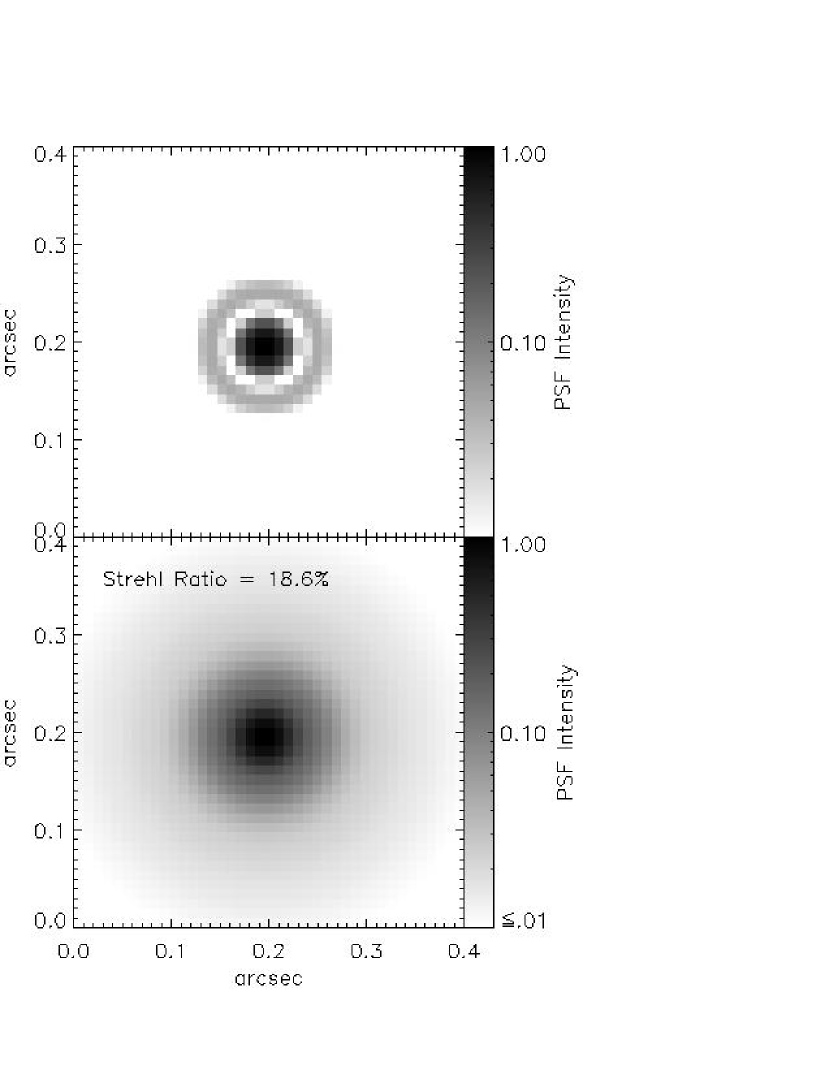
Figure 1 shows the resultant filtered and unfiltered atmospheric phase power spectra, phase structure functions, and associated MTFs. The filter function, $[1-H^{\prime}(\kappa)]^{2}$ in Eq. (3), suppresses the power spectrum at low frequencies. Figure 1 shows that the AO system has no effect on spatial scales smaller than the actuator spacing. The inability of the AO system to sense and correct for phase errors above the corresponding spatial frequency, along with its imperfect correction within the control bandwidth, prevents the final MTF from reaching the diffraction limited MTF. The resultant narrow MTF produces a PSF broadened from the diffraction-limited case with the familiar core-halo structure in PSFs delivered by AO systems (e.g., Hardy, 1998). The diffraction-limited PSF (no atmosphere) and the partially corrected case are shown in Figure 2. The PSFs shown are constructed by interpolating a highly oversampled PSF onto a grid appropriate for the NIRC2 camera. Though even a perfect, diffraction limited PSF must be sampled onto a pixel array, for the purposes of demonstrating change in Strehl ratio, the diffraction limited PSF shown has been constructed without taking the pixel MTF into account.

Figure 2: Model (azimuthally averaged) PSFs for Keck-AO/NIRC2 narrow camera ($0\farcs 01$ pixel^-1) displayed on a logarithmic grey scale. Both PSFs have been scaled so that their peak value is 1, i.e flux was not conserved. Top: the diffraction-limited PSF. Bottom: the partially-corrected PSF for $r_{0}=65$ cm, $L_{0}=30$ m, $\sigma_{DM}=56$ cm, and $w=1.5$. The Strehl ratio is 18.6%.

5 MTF Fitting and Photometry

5.1 Construction and fitting of simulated data

Using PSFs generated according to the recipe of § 4, we generate mock Keck images from which we then extract the MTF by fitting our model to the resultant image power spectrum. We evaluate the robustness of our approach by comparing the input and recovered parameters and we quantify photometric errors by evaluating the discrepancy between the model and reconstructed PSF and EE.

We consider three model PSFs with $r_{0}$ = 50, 65, and 100 cm, and common parameters $L_{0}$ = 30 m, $w$ = 1.5, and $\sigma_{DM}$ = 56 cm. Again, we ignore measurement noise by setting $\Delta^{2}_{\phi}=0$. To explore the effects of crowding, we populated images with 5, 50, 500, 5000, 50,000, and 5$\times$10⁶ stars in a field of view of $4\farcs\times 4\farcs$. The stars have random positions and normally distributed brightnesses. The final step of synthesizing a star field involves convolving the array of delta functions with the PSF. The heights of the delta functions are scaled to approximate the distribution of fluxes present in our data, and we add normally distributed noise to the images to represent detector read noise and Poisson sky noise so that the model images have similar signal-to-noise ratios as our observations. Some example model images are shown in Figure 3.

Figure 3: Model Keck-AO/NIRC2 images demonstrating the effects of different values of $r_{0}$ and numbers of stars, $N_{*}$. All images represent $H$-band data taken with the NIRC2 camera operating at the $0\farcs 01$ pixel^-1 platescale, and share the common parameters $L_{0}=30$ m, $w=1.5$, $\sigma_{DM}=56$ cm, and $\Delta_{\phi}^{2}=0$. (a) $r_{0}=50$ cm, $N_{*}$ = 50; (b) $r_{0}=65$ cm, $N_{*}$ = 50; (c) $r_{0}=1$ m, $N_{*}$ = 50; (d) $r_{0}=65$ cm, $N_{*}$ = 500; (e) $r_{0}=65$ cm, $N_{*}$ = 5000; (f) $r_{0}=65$ cm, $N_{*}$ = 5$\times$10⁶.

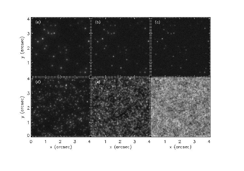
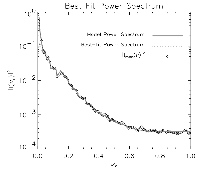
Figure 4 shows the measured power spectrum of the $N_{*}=50$, $r_{0}=65$ cm image from Figure 3(b). Also plotted is the model MTF (squared) used to generate the PSF multiplied by the input source distribution power spectrum, $|S(\nu)|^{2}$ as calculated from the array of delta functions used to construct the image. The model spectrum has been fit to the data using only a multiplicative normalization factor and an additive constant to represent the noise. Inspection of this plot suggests that it is reasonable that the MTF should be recoverable from astronomical data.

Figure 4: Measured, model, and best fit power spectra for the model image Figure 3(b) ($N_{*}$ = 50, $r_{0}=65$ cm). The open diamonds are the power spectrum extracted from the image; the solid grey line is the known power spectrum computed from the input data, consisting of the model MTF multiplied by the source distribution power spectrum of the original delta function array, and the constant noise floor; the dotted black line is the best fit power spectrum found after two iterations for StarFinder to estimate $|S_{mod}(\nu)|^{2}$.

Since our goal is to establish the unknown MTF for real astronomical data we test the ability of a non-linear least squares fit to recover the input parameters from simulated data. We use the IDL procedure MPFIT to perform a Levenberg-Marquardt least-squares fit of our model MTF to Eq. (7) using $|S_{mod}(\nu)|^{2}$ as an estimate of the source distribution power spectrum. Since we radially average the measured power spectrum, we are able to directly measure the error in each frequency bin by calculating the variance of each ensemble of pixels. We found that reliable error estimates were necessary to obtain unbiassed fits, especially when the AO correction was poor.

Figure 5: Comparison of the input encircled energy curves (diamonds) with the recovered encircled energy curves (solid) from the best fit MTF calculated from Eq. (A11) for a sample of model images. (a) $N_{*}$ = 50, $r_{0}=50$ cm; (b) $N_{*}$ = 50, $r_{0}=65$ cm; (c) $N_{*}$ = 50, $r_{0}=1$ m; (d) $N_{*}$ = 5, $r_{0}=50$ cm; (e) $N_{*}$ = 500, $r_{0}=50$ cm; (f) $N_{*}$ = 5000, $r_{0}=50$ cm.

The model function for $T_{sys}(\nu_{n})$ in Eq. 5 is calculated in steps. The transfer function $T_{pup}(\nu_{n})$ is calculated numerically from the Keck pupil as described in § 4. The pixel transfer function $T_{pix}(\nu)$ is calculated analytically from Eq. A9. Both $T_{pup}$ and $T_{pix}$ have no free parameters. $T_{\phi AO}(\nu)$ is, itself, calculated in steps. We first calculate the AO filtered atmospheric phase error power spectrum $|\Phi_{AO}(\kappa)|^{2}$ as given in Eq. 3, using Eq. 8 for the unfiltered atmospheric power spectrum and Eq. 10 in $H^{\prime}(\kappa)$. Calculating these quantities introduces the fit parameters $r_{0}$, $L_{0}$, $\sigma_{DM}$, $w$, and $\Delta_{\phi}$. The structure function is then constructed numerically using Eq. A4. (The numerical calculation of the structure function is by far the most computationally time consuming step, a problem compounded by the many iterations necessary of a non-linear least squares fit.) $T_{\phi AO}(\nu_{n})$ is then given by Eq. A7.

We consider $\sigma_{DM}$ a known quantity and hold it constant at 56 cm. We also neglect any wavefront measurement error and set $\Delta_{\phi}=0$. In addition, we fit for the multiplicative normalization constant of the term $|S_{mod}(\nu)|^{2}|T_{sys}(\nu)|^{2}$ and the noise in the image, $|N|^{2}$. These terms, however, do not affect the resulting PSF.

We estimate $|S_{mod}(\nu)|^{2}$ with a variety of methods. The first uses aperture photometry: for each image, we perform fits using the DAOPHOT routine FIND implemented in IDL to locate sources in the image and to estimate their relative fluxes. The second method is iterative: using the parameters determined from the FIND fits we generate a PSF and use this PSF with the crowded field photometry package StarFinder (Diolaiti et al., 2000) to again estimate the source function, hopefully more accurately. (Note, we use StarFinder only to determine the location and relative intensity of point sources, not to estimate the PSF.) We use parameters from this fit to generate a new PSF to use again with StarFinder in a subsequent iteration. The third method is used to investigate how well the fits work when analyzing model data and the source function is known perfectly: we compute $|S_{mod}(\nu)|^{2}$ directly from the array of delta functions that was used to construct the model image. In either case we create an array of size equal to the image and place delta functions in this array at the locations of the sources with heights equal to the fluxes. We radially binned and averaged the resultant 2-d power spectrum to obtain $|S_{mod}(\nu)|^{2}$. In order to leave the overall measured power unchanged, we normalize $|S_{mod}(\nu)|^{2}$ to have a median value of 1. $|S_{mod}(\nu)|^{2}$ is then an indication of how much $|S(\nu)|^{2}$ deviates from being a multiplicative constant. Finally, we also perform fits ignoring the correction for the source distribution power spectrum by setting $|S_{mod}(\nu)|^{2}=1$.

Figure 4 shows the best fit to the power spectrum for image Figure 3(b) ($N_{*}=50$, $r_{0}=65$ cm), after two StarFinder iterations. The final fitted MTFs are then used to compute the PSFs and encircled energy using Eq. A10 and A11. Some comparisons of the input and recovered EE curves are shown in Figure 5.

5.2 Comparison of input and recovered parameters

In general, the fits are insensitive to the model parameters for $r_{0}>$ 150 cm. For $r_{0}\gtrsim$ 2 m, the MTF becomes barely distinguishable from the perfect MTF. In this regime it becomes impossible to contrain any of the parameters. It is not surprising, therefore, that the fitted parameters for $r_{0}$ = 100 cm are less accurate than those for $r_{0}$ = 50 cm and 65 cm. This degradation in accuracy applies to the fitted parameters for all of the images, as reflected in their calculated formal errors, regardless of the number of stars in the field. However, in the case of high $r_{0}$, the encircled energy and PSF are less dependent on the model parameters, so the quantities of interest are left mostly unaffected.

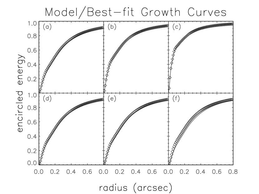
For images containing 500 stars or fewer, the recovered photometric growth curves deviate from the true values by less than 2%. The fits for the images containing five and fifty stars generally returned the input parameters to within the calculated error. The recovered encircled energy curves for these fits matched the input well, with the maximum deviations from the known growth curves less than 1.5%. The accuracy was much better than this for $r_{0}=65\;cm$ and $1\;m$. Estimating the source distribution power spectrum and accounting for it in the model improved the fits and was robust. Using simple DAOPHOT aperture photometry routine for this purpose was sufficient, as the separation between the stars was large. Signal to noise ratio plays a significant role in the accuracy of the fits. The five star images yielded less accurate fit parameters than the fifty star images. Since we did not hold the total flux constant when constructing images with different numbers of stars, we created additional five star images scaled to match the total signal in the fifty star images. Performing the fits on these new images yielded more accurate results, in line with those obtained from the fifty star images.

It is more difficult to estimate the source distribution power spectrum for the images with more than fifty stars because of increased crowding. Nonetheless, fitting the 500 star images returned parameters that were close to the input values when we used the iterative method to refine the estimate of the source distribution function. The resulting photometric growth curves, though less accurate than those for five and fifty stars, do not deviate from the known ones by more than 2%. Using the known source distribution function for these synthentic data yields improved fit parameters, confirming that with this many stars uncertainty in $|S_{mod}(\nu)|^{2}$ is the dominant source of error.

For the images containing $\geq$ 5000 stars, the accuracy of the returned parameters drops again. Nonetheless, the best-fit photometric curves of growth differ from the true ones by usually less than 5%. When a field contains so many stars that every beam contains multiple stars, estimating the spatial distribution power spectrum becomes impossible. In this case, we hope that the assumption of a random distribution of point sources leading to a simplification of $|S(\nu)|^{2}$ as a constant becomes increasingly valid. For the images containing 5000 stars ($\simeq$ 0.4 stars per $(\lambda/D)^{2}$ beam), the best fit parameters deviate significantly from the input parameters. The field is sufficiently crowded that errors in $|S_{mod}(\nu)|^{2}$ are large, but not so crowded that $|S(\nu)|^{2}$ may be approximated as a constant. The deviations in the fitted encircled energy from the true encircled energy are as great as 5%. These same problems apply to the images with 50,000 stars ($\simeq$ 4 stars per beam), but to a greater extent. In this regime, the fits almost completely fail to return the input parameters. Accurately estimating the source distribution here is almost impossible. The fits performed while considering $|S(\nu)|^{2}$ as a constant do not produce better results, indicating that the field is not random enough to allow this assumption.

The 5 $\times$ 10⁶ image ($\simeq$ 400 stars per beam) defies any attempt to estimate the source distribution function. However, in this limiting case, the field is so crowded that neglecting to account for $|S_{mod}(\nu)|$ does not cause the fits to fail. The fits, though not as accurate as those for the images with 5–500 stars, yield encircled energies no more than 6% different from the true curves.

Though poor sky subtraction degrades the accuracy of the fits, the effect can be mitigated by filtering out the low spatial frequency bins. We estimated the background directly from the model images and sky subtracted before finding the power spectrum. Since the sky subtraction will never be perfect and is, for the images with more than 500 stars, significantly inaccurate, the power spectrum is contaminated. However, if we assume that the background does not contain much power beyond the lowest few frequency bins, we can exclude these bins from our fits. (The first two frequency bins in Figure 4 demonstrate the effect of imperfect sky subtraction.) For the 5, 50, and 500 star images we ignored the first two frequency bins ($\nu_{n}<0.02$), which yielded more accurate results than using all data points. For the 5000 star image, we repeated the fits, filtering out the first three bins. This resulted in best-fit parameters somewhat closer to the inputs, but did not significantly improve the accuracy of the best fit EE curve.

In general, it appears that the benefits of increased signal to nosie in the images with large numbers of stars, as well as the benefits of the increased validity of the assumption of randomness in the source function, are outweighed by the increased ability to sky subtract and to estimate the source function in images with less crowding. (Assuming, of course, that there is enough signal to be able to use fewer stars.) For instance, the measured power spectra for the $N_{*}=5\times 10^{6}$ images are noisier than for those with 5, 50, and 500 stars, and the fitted parameters are consequently less accurate, even though the assumption of a random spatial distribution holds better for these images than for those with less stars and the signal to noise is much higher.

While our most crowded images ($N_{*}=5\times 10^{6}$) yielded fits less accurate than our least crowded images ($N_{*}\leq 500$), they still led to best-fit curves of growth that were accurate to $<$ 6%. There appears to be a regime, however, in which the field is not crowded enough to allow for the approximation of $|S(\nu)|^{2}$ as a constant, but too crowded to allow for an accurate estimation of it. Our example of this is the failed fits for images containing 50,000 stars. In this case, we were unable to find a satisfactory way to improve the fits.

5.3 Fitting laser guide star Keck AO data

The nearby dwarf starburst galaxy NGC 1569 ($v_{helio}$ = $-$104 km s^-1) was observed with the Keck LGS/AO and the NIRC2 camera on 2005 March 02. The field is centered on the superstar cluster SSC A1/A2 (Origlia et al., 2001). The NIRC2 pupil stop was in the LARGEHEX position (circumscribed circle) and the camera was operating in the narrow field mode ($0\farcs 01$ per pixel). Observing conditions were photometric, and the seeing was $0\farcs 4$ at $H$. The $R\simeq 11$ mag. equivalent laser guide star was projected at the center of the science camera field of view and SSC A1/A2 was used as the tip-tilt reference. The science field was observed at an airmass of 1.5 with the AO system running at 450 Hz. We use a 60-second $H$-band exposure from this observation to illustrate the application of our PSF estimation method. Additional observations with 120-s exposures were also obtained yielding a mosaic with a total exposure time of 15 minutes.

Figure 6: A 60 second Keck LGS AO NIRC2 $H$-band image of super-star cluster A in NGC 1569. An MTF was measured and fitted for the entire image and for the two indicated subarrays.

Flat-fields were taken at the zenith near midnight and median filtered to remove starlight. Bad pixels in the single 60-s image were repaired by substituting them with an interpolation of the surrounding pixels. As the crowding in the field is relatively low and displays little variation across the field, conventional sky subtraction was applied using the IDL implementation of the DAOPHOT routine MMM.

Figure 7: The measured power spectrum of the entire image in Fig. 6 and the best-fit model power spectrum based on the MTF and source distribution function. $\sigma$ is the rms error of the ensemble of pixels that was radially binned and averaged to produce the 1-d spectrum. The fit parameters are listed in the last column of Table 1. The corresponding encircled energy curve is shown in Fig. 8.

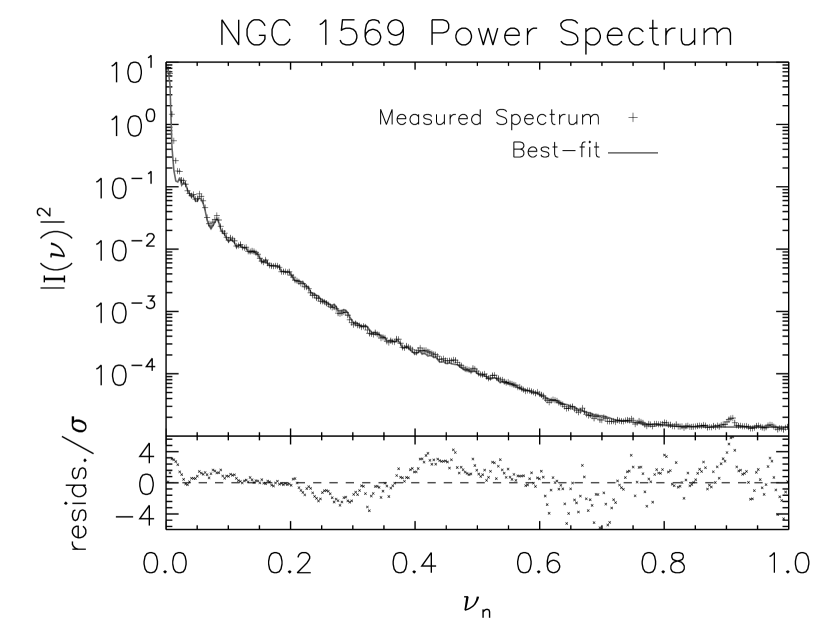
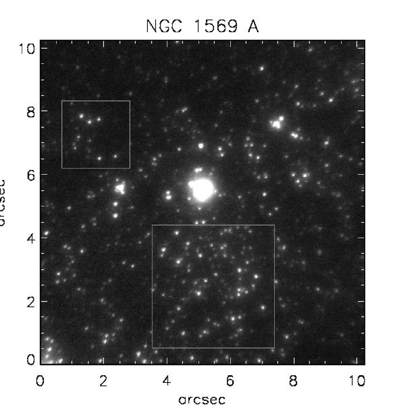
Figure 6 shows the entire NIRC2 field of view. The image is dominated by the resolved cluster but also includes several hundred unresolved stellar sources. The cluster light includes extended nebular emission and is therefore not suitable for measuring the MTF. Our goal is to estimate the PSF for the regions containing stars. Therefore, we define two subarrays within Fig. 6 that avoid SSC A and contain approximately 190 and 20 point sources, respectively. (Preliminary photometry indicates that the point sources in the image have absolute $H$-band magnitudes consistent with single red supergiant stars.) Anisoplanatism is evident in Fig. 6. We have chosen regions small enough ($\sim$ $2^{\prime\prime}\times 2^{\prime\prime}$ and $\sim$ $4^{\prime\prime}\times 4^{\prime\prime}$ ) so that this effect should be negligible. For comparison, we also compute the power spectrum for the entire image after masking out the central cluster and two other bright, unresolved objects.

Figure 8: The recovered encircled energy curve corresponding to the fitted power spectrum (see Fig. 7) of the entire image in Fig. 6. The fit parameters are listed in the last column of Table 1.

The best-fit power spectrum and encircled energy for the entire image are shown in Figures 7 and 8. The best-fit parameters are listed in Table 1 along with those for the fits using the two subarrays. We again hold $\sigma_{DM}$ at a constant 56 cm. All parameters represent the best-fit after two iterations of using StarFinder to estimate the source distribution power spectrum. We also state the formal errors in the parameters as computed from the covariance matrix. To account for any imperfect sky subtraction, we do not fit data at $\nu_{n}<0.02$. Thus we filter our spectra below the first 1, 2, and 5 frequency bins in the small and large subarrays, and in the entire image, respectively.

Figure 9: The PSF generated for the entire image’s best-fit parameters listed in Table 1.

In § 5.1 our model PSFs were circularly symmetric and based solely on our model MTF. All we verified there was the ability to successfully extract the MTF from data. Since real PSFs will contain asymmetries and since our model will not describe all of the factors contributing to an actual MTF (i.e., deviations from Kolmogorov turbulence, directional dependence in $D(r)$, systematic errors in the wavefront sensor) we cannot expect our real fits to be as accurate as our fake fits. Nevertheless, Figure 7 shows excellent agreement between measured and best-fit model power spectra—we have evidently included enough detail in our model to capture the essence of the Keck AO system. Based on the analysis of our synthetic data, the recovered values put us in the regime where the fits show good sensitivty to $r_{0}$ and $w$. Additionally, the three sets of fit parameters mostly agree to within the formal errors. The values of $L_{0}$ show some discrepancy, but in this region of model parameter space the MTF and EE show no signficant variation when $L_{0}$ changes by as much as 10%. The recovered EE curve is most sensitive to changes in $r_{0}$, which stays within error over the three fits. The density of stars in our image is low enough to enable accurate sky subtraction and estimation of the source distribution function. All of these factors give us confidence in our derived parameters.

Figure 10: Typical residuals after performing PSF subtraction on stars in Figure 6 using the PSF in Figure 9. All images are displayed on a linear scale and have a $1\farcs 50\times 1\farcs 50$ field of view. The residuals show mainly azithumal structure, an effect we may attribute mainly to the failings of our model to describe non-radially symmetric PSFs. Such residuals should have little effect on the encircled energy.

The formal errors decrease significantly as the size of the subarray we use to measure a power spectrum grows. For one, the signal to noise ratio of the power spectrum increases when there are more stars. Also, larger images give finer sampling of the power spectrum. For these reasons, and since the best-fit power spectrum for the whole 60-s image is a good quantitative match with the measured one and does not differ significantly from either two subarrays, we choose the entire image best-fit MTF to compute a PSF and EE curve.

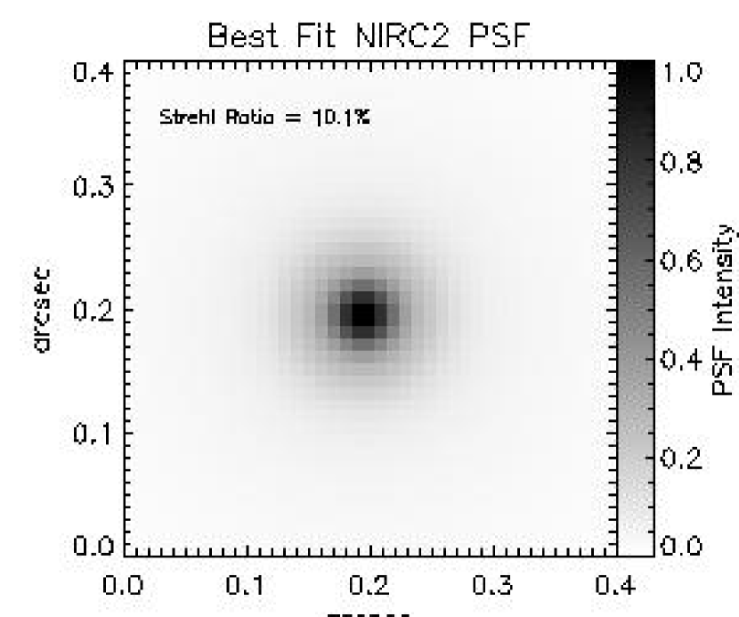
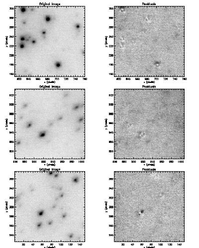
We use the best-fit parameters to generate an MTF and compute the corresponding PSF using Eq. (A10). The recovered PSF is shown in Figure 9. This PSF exhibits the same core-halo structure that is evident in the data. We performed PSF fitting and subtraction for a number of bright sources in the image. A few of the original stars and the residuals after PSF subtraction are shown in Figure 10. The residuals contain approximately $\pm 10\%$ of the original starlight, a failing that can probably be attributed to our initial assumptions about the symmetry of the PSF. Indeed, most of the residuals exhibit asymmetric structure. This indicates that the actual PSF’s deviation from circular symmetry, something for which our model is unable to account, is responsible for much of the residual starlight.

	$N_{*}$ $\simeq$ 20	$N_{*}\simeq$ 190	Full Image
$r_{0}\;(m)$	0.58 $\pm$ 0.09	0.56 $\pm$ 0.04	0.56 $\pm$ 0.02
$L_{0}\;(m)$	17.5 $\pm$ 1.0	20.0 $\pm$ 0.6	18.1 $\pm$ 0.2
$w$	1.33 $\pm$ 0.08	1.34 $\pm$ 0.04	1.33 $\pm$ 0.02

Table 1: Best fit parameters for the two sub-arrays indicated in Figure 6 and for the entire image.

5.4 Photometry

In this section we investigate the accuracy of photometry extracted from LGS/AO observations by comparing the results with data obtained using Hubble Space Telescope/NICMOS. The PSF for HST instruments is well characterized (e.g., Krist et al., 1998) hence the aperture corrections are known and HST data provide a good standard against which ground-based AO measurements can be compared.

Ideally, we would perform the LGS/AO photometry in two steps. First, perform relative photometry using PSF fitting with an empirical 2-d PSF, which is built from stars judged to be isolated. Second, use our 1-d PSF to compute the aperture corrections and place the relative photometry on an absolute scale. Since we are interested in the accuracy attainable with our method we have chosen to perform PSF fitting photometry with the model 1-d PSF obtained as described in § 5.3. While crowding will limit the precision of this approach, there is no ambiguity in how to calculate the aperture correction. When applied to an ensemble of stars this one-step method should give a reliable way of evaluating the accuracy of the resultant photometry.

Figure 11: The Keck AO image of NGC1569A and the corresponding sub-image of the NICMOS mosaic. The NICMOS image has been rotated to match the Keck field-of-view. The arrow indicates a variable star with the largest observed fluctuation ($\delta m$ = 0.8 mag.).

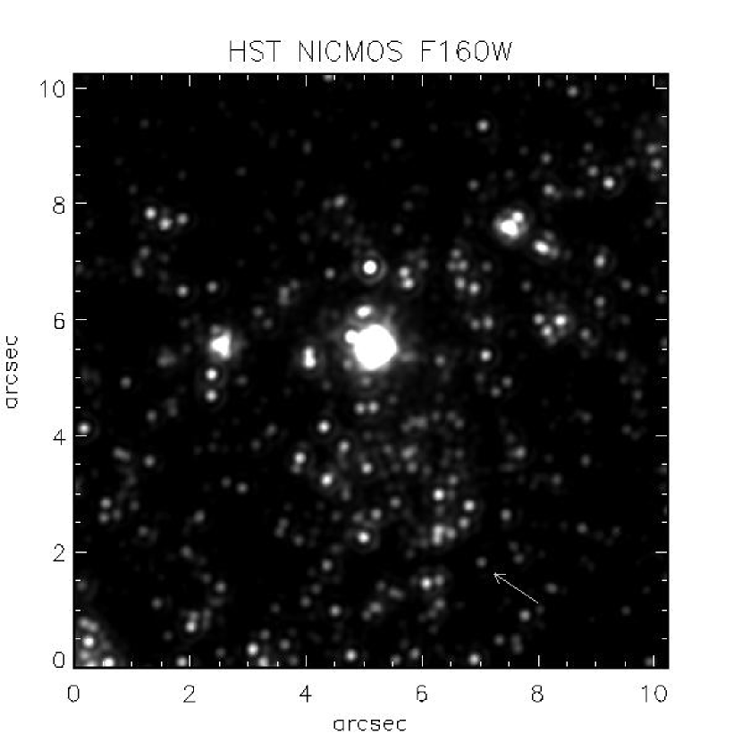
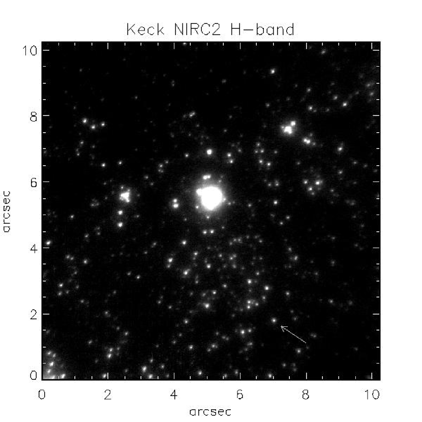
We measure $H$-band magnitudes for approximately 250 bright point sources in the field of a single 60-s exposure of NGC 1569 SSC A ($r_{0}$ = 56 cm; Strehl = 10.1%; see § 5.3). We used five images of the near-infrared standard star SJ 9139 (Persson et al., 1998) obtained on the same night as the science data to measure the photometric zero point.

Figure 12: The magnitudes for 243 stars common to the Keck and HST fields of view. The HST magnitudes were taken from Aloisi et al. (2001) and color corrected from the NICMOS F160W filter to Keck’s $H$ filter. The dashed line has slope 1 and intercept 0. The triangle is the star indicated by the arrows in Figure 11.

HST data were obtained with the NIC2 camera in the F160W filter on 1998 February 25. The Keck image and the matching NICMOS sub-image are shown side-by-side in Figure 11. Photometry for the HST/NICMOS images has been extracted by Aloisi et al. (2001). Comparison of the photometry obtained from our LGS/AO data begins with matching the catalogs of Keck and HST/NICMOS sources. Inspection of Figure 11 shows that Keck frequently resolves stars that appear as single sources to HST/NICMOS. Although we are able to identify more stars in the Keck image than presented here, we have selected only those stars that are separated from neighbors by more than $0\farcs 1$ in both catalogs. The central wavelengths of the NICMOS F160W filter (1.60 $\mu$m) and the NIRC2 $H$-band filter (1.63 $\mu$m) are similar. However, the filter bandpasses differ significantly, and for these red stars a color correction is necessary to compare space and ground-based measurements. We correct the HST F160W magnitudes to the Keck system based on their F160W-F110W colors, using the method outlined in the appendix of Marleau et al. (2000).

A plot of Keck vs. color-corrected HST magnitudes for isolated stars (Figure 12) shows that the mean photometric discrepancy between the two data sets amounts to only a few percent. In this figure the data points fall along a straight line of unit slope and intercept zero. The mean Keck magnitude minus the HST magnitude, $\delta m$, is $\overline{\delta m}$ = 0.05 mag., and standard deviation is $\sigma_{\delta m}$ = 0.21 mag. The standard error of $\delta m$ is 0.013 mag.

Figure 13: The difference between the measured 60-s Keck exposure magnitudes and the HST magnitudes as a function of distance from the center of the FOV. Anisoplanatism would appear as an error that increases with distance from the laser beacon (projected at $r=0$). The dashed line shows the best-fit second order polynomial, illustrating that there is only a weak trend in the photometric errors.

The agreement between the Keck and HST photometry at the 5% level is encouraging, and provides significant validation for our method of finding AO aperture corrections. However, the roughly 20% scatter for individual measurements, which is several times larger than that expected from source, sky and detector noise, merits some additional comment.

One possible source of scatter is anisoplanatism in the AO images. A systematic change in the PSF and across the field of view would result in seemingly random errors distributed among stars of all magnitudes in Figure 12. However, a plot of $\delta m$ vs. field angle (Figure 13) shows only a weak trend, and indicates that variation of the AO PSF across the Keck field of view only contributes a fraction ($\simeq$ 10%) of the 0.21 mag. scatter.

We investigate our internal errors by comparing two independent sets of LGS/AO observations of the field of NCG 1569 SSCA. For the first image we use the same 60-s exposure as above and a 120-s exposure for the second ($r_{0}$ = 42 cm; Strehl = 3.7%. Each image has a different PSF and a sky background level. Comparing the photometry done from the 60s and 120s exposures gives $\overline{m_{60s}-m_{120s}}=0.04$ mag. and $\sigma_{(m_{60s}-m_{120s})}=0.10$ mag. Thus, our measurement errors account for only about 20% of the variance between the Keck and HST.

Likely, the major source of the observed scatter is the natural variability of red supergiants (RSGs), the main stellar component present in this field. Visual inspection of the NIRC2 and NICMOS images reveal several stars that have brightened or dimmed betweeen 1998 and 2005. The most variable star, with $\delta m=0.8$, is indicated by the triangle in Figure 12 and the arrow in Figure 11. The magnitudes and F160W-F110W colors ($\approx 1$) of our sample indicate they are mostly RSGs with masses $\gtrsim 10M_{\odot}$ (Aloisi et al., 2001). The most massive few stars are probably between $20M_{\odot}$ and $30M_{\odot}$. The stars in our sample are unstable and can fluctuate significantly in luminosity. Maeder (1980) has studied this variability in a sample of 2420 RSGs. The results indicate that stars of these masses and spectral types have average peak-to-trough $V$-band amplitudes between 0.1 for $10M_{\odot}$ stars and 0.4-0.8 for $30M_{\odot}$ stars. Although the amplitude of variation is likely to be less at infrared wavelengths, these findings suggest that we can attribute most of the observed variance to the stars themselves.

Since the 120-s exposure exhibited poorer image quality, it affords the opportunity to examine the photometric integrity for reduced AO correction. The same photometric Keck-HST comparison for these data give $\overline{\delta m}=-0.03$ mag. and $\sigma_{\delta m}=0.23$ mag., confirming that accurate results can be extracted at low Strehl ratios.

6 Discussion

We have developed a simple model to describe the imaging performance of an AO system. The model makes assumptions about the shape of the power spectrum of atmospheric phase errors, the pupil geometry, and the DM influence function and has a few adjustable parameters, including the Fried parameter ($r_{0}$), the degree of AO correction ($w$), and the wavefront measurement noise ($\Delta\phi$). Beyond the inherent value of a well defined framework to quantify an observed phenomenon, this method has several advantages in the practical analysis of AO data. Generating numerical MTFs is a cheap and easy way to predict system performance under a variety of conditions, i.e., seeing, pupil obscuration, DM actuator spacing, &c.

By considering the Fourier information present in astronomical images we have shown that it is practical to fit model MTFs to image power spectra, constrain the model parameters and recover the PSF, encircled energy and Strehl ratio. High fidelity simulations of AO performance can be performed using computationally intensive Monte Carlo codes (e.g., Jolissant, 2004). However, we believe that we have shown that it is unnecessary to employ these elaborate methods to compare with observations to estimate photometric curve of growth corrections.

Using the method outlined here, the azimuthally averaged PSF and hence the photometric curve of growth can be estimated directly from an image containing multiple point sources. Data obtained in varying observing conditions and with changing AO correction can be analyzed so that they are not subject to systematic photometric errors, and separate and potentially unreliable PSF star observations are not required. Our method allows one to estimate the PSF, even if there are no isolated stars in the image. Although only the azimuthally averaged PSF is derived, the fact that the residuals in Figure 10 show mainly azimuthal components means that the curve of growth is valid. A comparison of Keck LGS/AO and HST/NICMOS observations of the same field at 1.6 $\mu$m in NCG 1569 shows that our photometric method is accurate to 5% or better. The precision of our 1-d PSF fitting photometry (about 10%) is not limited by photon statistics and detector noise. We are investigating a hybrid approach which involves conventional 2-d PSF fitting photometry using an empirical kernel followed by application of aperture corrections derived from MTF fitting.

Treating the OTF as a one-dimensional MTF is an approximation. The wavefront delivered by an AO system often suffers from systematic calibration errors which lead to significant PSF azimuthal asymmetry. Non-circular pupils and anisotropic atmospheric turbulence, e.g., due to a prevailing wind, are the rule rather than the exception. While odd-order aberrations, e.g., coma, cannot be reconstructed from the power spectrum, even aberrations like astigmatism can be described. A natural extension to the work presented here is to fit a 2-d OTF to the 2-d power spectrum to capture this information. It will be particularly interesting to investigate the ability of this method to describe the astigmatism introduced by angular anisoplanatism by mapping out the variation of model parameters as a function of field angle.

Appendix A Appendix: Modulation Transfer Functions

The optical transfer function (OTF) specifies the amplitude and phase response of a linear optical imaging system to a stimulus at a given spatial frequency. In general the OTF is complex. Here we consider the special case of a circularly symmetric PSF, in which case the complex OTF reduces to the real modulation transfer function (MTF). Following Schroeder (2000), the MTF, $T(\nu)$, is a measure of the contrast at spatial frequency $\nu$ in the image, relative to the object. We expect $T(\nu)\rightarrow 1$ as $\nu\rightarrow 0$. For a pupil with finite support, above some critical spatial frequency, $\nu_{c}$, $T(\nu_{c})=0$ and all information at frequencies greater than $\nu_{c}$ is lost.

In the image plane, the cutoff spatial frequency of a telescope with a circular pupil, diameter, $D_{tel}$, and observing wavelength, $\lambda$, is

$$\nu_{c}=1/F\lambda.$$ (A1)

This corresponds to a linear image size of $f\lambda/D_{tel}=F\lambda$, where $f$ is the effective focal length at the image plane and $F=f/D_{tel}$ is the focal ratio. It is convenient to use spatial frequencies in units of the cutoff frequency in the image plane, or normalized spatial frequencies, $\nu_{n}=\nu/\nu_{c}=\nu\lambda F$.

A.1 Atmospheric MTF

The variation in phase of a wavefront, $\phi$, between two points in the pupil plane of a telescope separated by a distance $\mathbf{r}=\mathbf{r}_{1}-\mathbf{r}_{2}$ can be described by the structure function

$$D_{\phi}(\mathbf{r})=\langle[\phi(\mathbf{r}_{1})-\phi(\mathbf{r}_{2})]^{2}\rangle,$$ (A2)

where $\langle...\rangle$ denotes a time average. We reserve lower case, e.g., $\phi$, to refer to quantities in the spatial domain, and upper case, e.g., $\Phi$, for the Fourier transformed quantity in the frequency domain. We use $\mathbf{x}$ and $\nu$ to refer to spatial coordinates and spatial frequencies in the image plane and $\mathbf{r}$ and $\kappa$ to refer to spatial coordinates and spatial frequencies in the pupil plane. Thus, the relation between position in the pupil plane and spatial frequency in the image plane is $\mathbf{r}=\lambda f\mbox{\boldmath$\nu$}$.

The structure function can be written in terms of the covariance function, which in turn forms a Fourier pair with the two-dimensional phase-error power spectrum, $|\Phi(\mbox{\boldmath$\kappa$})|^{2}$, where $\kappa$ is spatial frequency in the pupil plane. The notation $|\Phi|^{2}$ denotes the atmospheric phase error power spectrum, which is shorthand for the expectation value $\langle\Phi\Phi^{*}\rangle$, where $*$ denotes the complex conjugate. Consequently, the structure function and the power spectrum are related by the transform

$$D_{\phi}(\mathbf{r})=2\int|\Phi(\mbox{\boldmath$\kappa$})|^{2}[1-\cos(2\pi\mathbf{\mbox{\boldmath$\kappa$}\cdot r})]d\mbox{\boldmath$\kappa$},$$ (A3)

where the integral is taken over the infinite domain. In the case of an isotropic power spectrum integration over the angular part yields

$$D_{\phi}(r) = 2\int_{0}^{\infty}|\Phi(\kappa)|^{2}\;\kappa d\kappa\int_{0}^{2\pi}d\theta\;[1-\cos(2\pi\;kr\cos\theta)]$$ (A4)

$$= 4\pi\int_{0}^{\infty}|\Phi(\kappa)|^{2}[1-J_{0}(2\pi\;\kappa r)]\kappa\;d\kappa,$$

where $\kappa=|\mbox{\boldmath$\kappa$}|$ (Tatarski, 1961), and $J_{0}$ is the Bessel function of the first kind. Note that this transform, as quoted by (Hardy, 1998, Eq. 4.46), contains a typographical error.

For Kolmogorov turbulence, with an infinite outer scale and an inner scale of zero, the two dimensional phase error power spectrum in the pupil plane is

$$|\Phi(\kappa)|^{2}=0.0229\;r_{0}^{-5/3}\kappa^{-11/3}$$ (A5)

(Noll, 1976). The corresponding phase structure function is

$$D_{\phi}(r)=6.88\left(\frac{r}{r_{0}}\right)^{5/3},$$ (A6)

where $r$ is the separation between two points in the pupil plane and $r_{0}$ is a scale length known as the Fried parameter (Fried, 1965). The phase structure function evaluated at $r=\lambda f\nu=D_{tel}\nu_{n}$ yields the atmospheric MTF structure function

$$T_{\phi}(\nu_{n})=\exp\left[\textstyle-\frac{1}{2}D_{\phi}(D_{tel}\nu_{n})\right]$$ (A7)

(Fried, 1966).

A.2 MTF of an unaberrated pupil

In the case of a unaberrated, unobscured, circular pupil, the OTF reduces to the real, circularly symmetric MTF,

$$T_{pup}(\nu_{n})=\frac{2}{\pi}\left[\cos^{-1}\nu_{n}-\nu_{n}(1-\nu_{n}^{2})^{1/2}\right].$$ (A8)

In the more general case of a pupil function with central obscuration, secondary spiders and segment gaps, the MTF can be computed numerically from the autocorrelation of the pupil function.

A.3 MTF of an ideal pixel

The MTF of a ideal pixel of dimensions $a\times a$ can be derived by considering it as a uniformly illuminated square aperture. The MTF is then given by the Fourier transform of this function, which in normalized frequencies is

$$T_{pix}(\nu_{n})=\mbox{sinc}(\pi\nu_{n}/n_{\rm pix}),$$ (A9)

where $n_{\rm pix}$ is the number of pixels per length $\lambda F$. For Nyquist sampling, two pixels per $\lambda F$, $n_{\rm pix}=2$. For the narrow field camera in Keck/NIRC2 $n_{\rm pix}=3.4$ at $H$ band.

A.4 PSF, encircled energy, and Strehl ratio

The final step involves finding the PSF, $p(r_{n})$, and the encircled energy, $e(r_{n})$, from the Hankel transforms of the system MTF $T_{sys}(\nu_{n})=T_{\phi}(\nu_{n})T_{pup}(\nu_{n})T_{pix}(\nu_{n})$. The Hankel transform of zero order yields the PSF,

$$p(r_{n})=2\pi\int_{0}^{1}T_{sys}(\nu_{n})J_{0}(2\pi\nu_{n}r_{n})\nu_{n}\;d\nu_{n}$$ (A10)

where $r_{n}=r/F\lambda=\theta D_{tel}/\lambda$ is the normalized distance in the image plane, and the Hankel transform of first order yields the the encircled energy

$$e(r_{n})=\int_{0}^{r_{n}}p(r^{\prime}_{n})\;2\pi r^{\prime}_{n}\;dr^{\prime}_{n}=2\pi r_{n}\int_{0}^{1}T_{sys}(\nu_{n})J_{1}(2\pi r_{n}\nu_{n})\;d\nu_{n}.$$ (A11)

where $J_{0}$ and $J_{1}$ are the Bessel functions of the first and second kind, respectively. The Strehl ratio is defined as $p_{sys}(0)/p_{pup}(0)$, where $p_{pup}$ denotes the PSF for the unaberrated system. Thus, using Eq. (A10)

$$S=\frac{\displaystyle\int_{0}^{1}T_{sys}(\nu_{n})\nu_{n}\;d\nu_{n}}{\displaystyle\int_{0}^{1}T_{pup}(\nu_{n})\nu_{n}\;d\nu_{n}}.$$ (A12)

References

- Aloisi et al. (2001) Aloisi, A., Clampin, M., Diolaiti, E., Greggio, L., Leitherer, C., Nota, A., Origlia, L., Parmeggiani, G., & Tosi, M. 2001, AJ, 121, 1425
- Carson et al. (2005) Carson, J. C., Eikenberry, S. S., Brandl, B. R., Wilson, J. C., & Hayward, T. L. 2005, AJ, 130, 1212
- de Pater et al. (2004) de Pater, I., Marchis, F., Macintosh, B. A., Roe, H. G., Le Mignant, D., Graham, J. R., & Davies, A. G. 2004, Icarus, 169, 250
- Diolaiti et al. (2000) Diolaiti, E., Bendinelli, O., Bonaccini, D., Close, L., Currie, D., & Parmeggiani, G. 2000, A&AS, 147, 335
- Fitzgerald & Graham (2006) Fitzgerald, M. P., & Graham, J. R. 2006, ApJ, 637, 541
- Fried (1965) Fried, D. L. 1965, Optical Society of America Journal A, 55, 1427
- Fried (1966) —. 1966, Optical Society of America Journal A, 56, 1372
- Hardy (1998) Hardy, J. W. 1998, Astronomical Adaptive Optics (Oxford University Press, New York)
- Herriot et al. (2000) Herriot, G., Morris, S., Anthony, A., Derdall, D., Duncan, D., Dunn, J., Ebbers, A. W., Fletcher, J. M., Hardy, T., Leckie, B., Mirza, A., Morbey, C. L., Pfleger, M., Roberts, S., Shott, P., Smith, M., Saddlemyer, L. K., Sebesta, J., Szeto, K., Wooff, R., Windels, W., & Veran, J.-P. 2000, in Proc. SPIE Vol. 4007, p. 115-125, Adaptive Optical Systems Technology, Peter L. Wizinowich; Ed., 115–125
- Jefferies & Christou (1993) Jefferies, S. M., & Christou, J. C. 1993, ApJ, 415, 862
- Jolissant (2004) Jolissant, L. 2004, PAOLA Simulation Software (http://cfao.ucolick.org/software/paola.php)
- Krist et al. (1998) Krist, J. E., Golimowski, D. A., Schroeder, D. J., & Henry, T. J. 1998, PASP, 110, 1046
- Linfield et al. (2001) Linfield, R. P., Colavita, M. M., & Lane, B. F. 2001, ApJ, 554, 505
- Maeder (1980) Maeder, A. 1980, A&A, 90, 311
- Marleau et al. (2000) Marleau, F. R., Graham, J. R., Liu, M. C., & Charlot, S. 2000, AJ, 120, 1779
- Max et al. (2005) Max, C. E., Canalizo, G., Macintosh, B. A., Raschke, L., Whysong, D., Antonucci, R., & Schneider, G. 2005, ApJ, 621, 738
- Melbourne et al. (2005) Melbourne, J., Wright, S. A., Barczys, M., Bouchez, A. H., Chin, J., van Dam, M. A., Hartman, S., Johansson, E., Koo, D. C., Lafon, R., Larkin, J., Le Mignant, D., Lotz, J., Max, C. E., Pennington, D. M., Stomski, P. J., Summers, D., & Wizinowich, P. L. 2005, ApJ, 625, L27
- Minowa et al. (2005) Minowa, Y., Kobayashi, N., Yoshii, Y., Totani, T., Maihara, T., Iwamuro, F., Takami, H., Takato, N., Hayano, Y., Terada, H., Oya, S., Iye, M., & Tokunaga, A. T. 2005, ApJ, 629, 29
- Noll (1976) Noll, R. J. 1976, Optical Society of America Journal A, 66, 207
- Origlia et al. (2001) Origlia, L., Leitherer, C., Aloisi, A., Greggio, L., & Tosi, M. 2001, AJ, 122, 815
- Perrin et al. (2004) Perrin, M. D., Graham, J. R., Kalas, P., Lloyd, J. P., Max, C. E., Gavel, D. T., Pennington, D. M., & Gates, E. L. 2004, Science, 303, 1345
- Persson et al. (1998) Persson, S. E., Murphy, D. C., Krzeminski, W., Roth, M., & Rieke, M. J. 1998, AJ, 116, 2475
- Rousset et al. (2000) Rousset, G., Lacombe, F., Puget, P., Gendron, E., Arsenault, R., Kern, P. Y., Rabaud, D., Madec, P.-Y., Hubin, N. N., Zins, G., Stadler, E., Charton, J., Gigan, P., & Feautrier, P. 2000, in Proc. SPIE Vol. 4007, p. 72-81, Adaptive Optical Systems Technology, Peter L. Wizinowich; Ed., 72–81
- Schroeder (2000) Schroeder, D. J. 2000, Astronomical Optics (Academic Press, San Diego)
- Sorrente et al. (2001) Sorrente, B., Cassaing, F., Rousset, G., Robbe-Dubois, S., & Rabbia, Y. 2001, A&A, 365, 301
- Stetson (1987) Stetson, P. B. 1987, PASP, 99, 191
- Strohbehn (1968) Strohbehn, J. W. 1968, Proceedings of the IEEE, 56, 1301
- Tatarski (1961) Tatarski, V. I. 1961, Wave Propagation in a Turbulent Medium (McGraw-Hill, New York)
- van Dam et al. (2004) van Dam, M. A., Le Mignant, D., & Macintosh, B. A. 2004, Applied Optics, 43, 5452
- Véran (1997) Véran, J. P. 1997, Ph.D. Thesis
- Wizinowich et al. (2004) Wizinowich, P. L., Le Mignant, D., Bouchez, A., Chin, J., Contos, A., Hartman, S., Johansson, E., Lafon, R., Neyman, C., Stomski, P., Summers, D., & van Dam, M. A. 2004, in Advancements in Adaptive Optics. Edited by Domenico B. Calia, Brent L. Ellerbroek, and Roberto Ragazzoni. Proceedings of the SPIE, Volume 5490, pp. 1-11 (2004)., 1–11