On the Evolutionary History of Stars and their Fossil Mass and Light

Abstract

The total extragalactic background radiation can be an important test of the global star formation history (SFH). Using direct observational estimates of the SFH, along with standard assumptions about the initial mass function (IMF), we calculate the total extragalactic background radiation and the observed stellar density today. We show that plausible SFHs allow a significant range in each quantity, but that their ratio is very tightly constrained. Current estimates of the stellar mass and extragalactic background are difficult to reconcile, as long as the IMF is fixed to the Salpeter slope above $1\,M_{\sun}$. The joint confidence interval of these two quantities only agrees with that determined from the allowed range of SFH fits at the $3\sigma$ level, and for our best-fit values the discrepancy is about a factor of two. Alternative energy sources that contribute to the background, such as active galactic nuclei (AGN), Population III stars, or decaying particles, appear unlikely to resolve the discrepancy. However, changes to the IMF allow plausible solutions to the background problem. The simplest is an average IMF with an increased contribution from stars around 1.5–$4\,M_{\sun}$. A “paunchy” IMF of this sort could emerge as a global average if low mass star formation is suppressed in galaxies experiencing rapid starbursts. Such an IMF is consistent with observations of star-forming regions, and would help to reconcile the fossil record of star formation with the directly observed SFH.

1 INTRODUCTION

In the last decade, observations have built up a picture of when and where stars form in the universe. From inventories of the stellar content of the local universe (Cole et al., 2001; Bell et al., 2003) and surveys of star formation over its entire cosmic history (e.g. Madau et al., 1996; Gabasch et al., 2004), it appears that star formation was much more rapid in the past, reaching a gentle peak at $z\sim\!1$–3 and falling off towards higher redshifts. These general trends are in accord with the $\Lambda$-dominated cold dark matter (LCDM) model of structure formation that has become widely accepted in recent years. This model successfully explains the spectrum of perturbations in the microwave background, the clustering properties of local galaxies, the optical depth and fluctuation spectrum of the Ly$\alpha$ forest gas, and the flux from distant supernovae (Spergel et al., 2006). However, galaxy formation is less well understood than these other phenomena. Theoretical models of galaxy formation can be implemented either by using semi-analytic calculations (e.g. Kauffmann et al., 1999; Cole et al., 2000; Somerville, Primack, & Faber, 2001) or by direct numerical simulations (e.g. Katz et al., 1992; Springel & Hernquist, 2003); each method has its own well-known advantages and drawbacks. Difficult issues that affect the results in both methods include galaxy supernova and AGN feedback (Springel et al., 2005; Dekel & Birnboim, 2006), the history and physical influence of reionisation (Gnedin, 2000; Bullock et al., 2000), the influence of “cold mode” accretion (Kereš et al., 2005), and the properties of zero-metallicity stars (Tumlinson et al., 2004). Different assumptions about these issues can produce quite different histories of star formation, so figuring out the total amount of star formation is a vital clue to the physics.

The observational measures of star formation are sufficiently imprecise that cross-checks using different measures are important. The star formation history (SFH) is measured by the direct emission from young stars or reprocessed radiation from dusty star-forming regions. This can be tested against the evolution of the stellar mass, using light from old stars (preferably in the near-infrared) as a proxy for mass; this has been carried out by many authors (e.g., Cole et al., 2001; Dickinson et al., 2003; Gwyn & Hartwick, 2005; Hopkins & Beacom, 2006). The integrated star formation rate tends to exceed the observed stellar mass, especially at high redshift. Given the large statistical and calibration errors in both quantities, however, the evidence for a discrepancy is not very strong. The observed metal density can be used as well (Madau & Pozzetti, 2000; Hopkins & Beacom, 2006), though the results from this approach are not yet precise enough to indicate more than a very approximate agreement. Hopkins & Beacom (2006) introduced the use of neutrinos from Type II supernovae to place an upper limit on the normalisation of the star formation history. Uncertainties in the effective neutrino temperature and stellar mass thresholds of Type II SNe cause systematic uncertainties in this limit; with present data, it is probably best to view the limit as constraining the supernova physics given the estimated SFH.

The extragalactic background light constitutes another vital test of the star formation history, since it records the total stellar emission over all time, weighted by the scale factor at the time of emission. The observed background light contains two humps, one in the far infrared (FIR) and one in the ultraviolet (UV) to near-infrared (NIR) range. The FIR hump primarily owes to thermal dust emission from heavily obscured, rapidly star-forming galaxies. There is much debate over the optical/NIR portion, in which the sum of the observed galaxies amounts to $\la 50$% of the total detected background (Wright, 2001; Bernstein, Freedman, & Madore, 2002a). The observed spectrum in this region might contain a hint of Lyman-$\alpha$ emission from low-metallicity, high-mass Pop III stars at $z>6$ (Matsumoto et al., 2005), but observational uncertainties and theoretical difficulties make this idea very controversial. It is certainly possible that most of the excess optical/NIR background light comes from the outer regions of normal galaxies or stars in faint undetected galaxies (Bernstein, Freedman, & Madore, 2002b).

Many authors have attempted to tie the background radiation in different wavebands to the history of specific subsets of galaxies, e.g. FIR emission from dusty starbursts or the NIR emission from pre-reionisation epoch galaxies. Madau & Pozzetti (2000) were the first to consider the total amount of the background radiation as a record of the cumulative stellar emission from all types of galaxies. This exercise is valuable because reprocessing of stellar radiation by dust and atomic continuum opacity, which can be very difficult to model correctly, will in general not significantly change the total amount of emitted energy. The stellar background energy is dominated by the stars that have already evolved off the main sequence, down as low as $0.9\,M_{\sun}$, so it samples a broader range of stellar masses than the direct indicators of the SFH. Madau & Pozzetti (2000; see also Madau et al., 2001, Pozzetti & Madau, 2001) found good agreement between the background radiation and the total amount of stars in the universe, concluding that there was little room for alternative sources of energy such as an early generation of stars with a top-heavy IMF. Since the work of Madau & Pozzetti, additional measurements of the background have been made in several different bands, and our understanding of the star formation history and local stellar density has improved. It thus seems worthwhile to test the background radiation as an indicator of the star formation history once more.

In §2, we discuss how we calibrate various indicators of the stellar mass and the star formation rate, and discuss the range of masses contributing to each. In §3, we discuss the observed cosmological background radiation, star formation history, and stellar mass density in the universe and we construct an ensemble of fits to the SFH to test the sensitivity of other observables to it. In §4, we compare the results of these various indicators of star formation to one another. Using the ensemble of star formation histories, we conclude that it is difficult to reconcile the background radiation with the stellar mass density observed today, using our default IMF assumptions. §5 discusses several possible solutions to this problem, focusing on the role of the stellar IMF. We show that the observed ratio of the total background light to the present-day NIR luminosity density is a powerful test of the IMF. Despite the large observational uncertainties, we can significantly restrict the allowed set of IMFs. §6 summarises our conclusions.

Since the IMF figures in every stage of our analysis and emerges as a focal point of our discussion, it is worth making a few introductory comments about its role. Indicators of the instantaneous star formation rate are dominated by massive stars; in our standard calculations below, for example, half of the UV luminosity comes from stars with mass $M\ga 15\,M_{\sun}$. The contribution of a stellar population to the extragalactic background depends on the integrated bolometric luminosity over its lifetime. This includes a significant contribution from less massive stars, and in our standard calculations half of the background comes from stars with mass $M>3M_{\odot}$. The present $K$-band light density comes largely from sub-giants and giants with masses just above the main-sequence turnoff, typically $M\sim 1M_{\odot}$ for an old stellar population. The expected ratio of these three measures of the cosmic star formation history, therefore, depends on the shape of the IMF above $1M_{\odot}$. Much of the mass in the IMF resides in low mass stars, and there has been a great deal of observational investigation of the IMF shape below $1M_{\odot}$. However, low mass stars emit very little light, so IMF changes in this regime have almost no impact on the relative values of these three probes of the cosmic star formation history; they change the expected/inferred stellar mass density for the three measures by the same factor. Our conclusions in this paper are, therefore, almost entirely insensitive to the adopted shape of the IMF below $\sim 0.8M_{\odot}$.

Throughout this paper, we assume a flat “737” LCDM cosmology of $\Omega_{M}=0.3$, $\Omega_{\Lambda}=0.7$, $h\equiv H_{0}/(100\,\mbox{km}\,\mbox{s}^{-1}\,\mbox{Mpc}^{-1})=0.7$, and $\Omega_{b}=0.02\,h^{-2}$, consistent with values derived from the WMAP experiment (Spergel et al., 2006).

2 CALIBRATIONS OF STELLAR ENERGY OUTPUT

Table 1: Initial Mass Functions

Forma	$K$	$x$	$M_{l}$	$M_{u}$
Salpeter	0.172	1.35	0.1	100
diet Salpeter	0.218	1.35	0.188	100
Kennicutt	0.328	0.4	0.1	1
	0.328	1.5	1	100
Miller-Scalo	0.354	0.4	0.1	1
	0.354	1.5	1	10
	2.02	2.3	10	100
Kroupa 1993	0.579	0.3	0.1	0.5
	0.310	1.2	0.5	1
	0.310	1.7	1	100
Chabrier	$\cdots$	$\cdots$	0.1	1
	0.238	1.3	1	100
Kroupa 2001	0.449	0.3	0.1	0.5
	0.224	1.3	0.5	100
Baldry & Glazebrook	0.323	0.5	0.1	0.5
	0.199	1.2	0.5	100
Paunchy	0.315	0	0.1	0.5
	0.194	0.7	0.5	4.0
	0.676	1.6	4.0	100
Obese	0.083	1.35	0.188	100
	0.905	1.65	1.5	100
Extreme top-heavy	0.136	0.95	0.1	100

^a The IMF is written as ${d\mathcal{N}}/{d\ln M}=K({M}/{\,M_{\sun}})^{-x}$, for $M_{l}<M<M_{u}$. The Chabrier IMF has a lognormal form $dN/d\ln(M)\propto\exp[-(\log(M/0.08))^{2}/(2\cdot 0.69^{2})]$ below $1\,M_{\sun}$, and is continuous at $1\,M_{\sun}$. In some cases the original versions of the IMF continued to lower mass, but we have imposed a uniform lower mass limit of $0.1\,M_{\sun}$.

In the central parts of some galaxies, the mass in stars can be estimated directly from its dynamical effects, but on larger scales the dynamics are dominated by dark matter. Hence, at present, all direct estimates of the global production of stars are based on the light they produce. The calibration of the mass-to-light ratio is sensitive to the age and metallicity of the population, but these can be constrained using the observed colours and/or spectral lines. The other major uncertainty is the stellar initial mass function (IMF). The most conventional choice is the original Salpeter IMF, with a mass range 0.1–$100\,M_{\sun}$. However, there is evidence that this contains too many low-mass stars, as shown both by local field star observations (Gould, Bahcall, & Flynn, 1996) and by estimates of the dynamical mass in ellipticals (Bell & de Jong, 2001). The latter authors advocate a “diet” Salpeter IMF, which they create by truncating the IMF at the low end so that it contains 0.7 times the mass in the current stellar population, when normalised to the same high-end amplitude. Using a representative estimate of the cosmic star formation history from our best fit below, we find that this implies 0.788 times as much mass in the IMF before the high-mass stars burn away; the indicators of star formation rate per mass of stars formed are thus shifted by the inverse of this factor. (This scaling is not very sensitive to the history.) These two IMFs and some other forms that we consider later in this paper are summarised in Table 1.

To convert between the star formation history and observed measures such as the stellar mass, UV continuum, and $K$-band light, we use the PEGASE.2 stellar population code (Fioc & Rocca-Volmerange, 1997). This code contains a large number of options for the stellar physics. Our conversions assume a close binary mass fraction of 0.05, evolutionary tracks with stellar winds, the SNII model B of Woosley and Weaver (1995), and a constant metallicity of $Z=0.02$. To assess the sensitivity of our results to this particular stellar population code, we have compared them to those obtained using the GALEXEV-2003 code of Bruzual & Charlot, and find only small differences of $\sim\!10$% at most (see also Bruzual & Charlot 2003, where some additional comparisons between the codes are presented).

Table 2: Conversion Factors for Star Formation Rate Indicators

IMF	$10^{7}$	$10^{8}$	$10^{9}\,\mbox{yr}$	$10^{7}$	$10^{8}$	$10^{9}\,\mbox{yr}$	$(10^{41}\mbox{erg}\,\mbox{s}^{-1}\,M_{\sun}^{-1}\,\mbox{yr})$
Salpeter	4.31	6.51	8.60	5.00	7.68	8.76	1.22
Diet Salpeter	5.52	8.33	11.0	6.35	9.75	11.1	1.55
Kennicutt	4.94	8.05	11.50	5.78	9.64	11.4	1.30

When constructing the cosmic SFH one needs to convert from observed luminosity to star formation rate (SFR). Table 2 lists the conversion factors of different star formation indicators for three different IMFs. The conversion factors are $f_{bol}\equiv L_{bol}/{\it SFR}$, $f_{H\alpha}\equiv L_{H\alpha}/{\it SFR}$, and $f_{UV}\equiv L_{\nu}/{\it SFR}$. The latter quantity is nearly constant over the wavelength range 1500–2800 Å used in various UV galaxy surveys, since $L_{\nu}$ itself is nearly constant before extinction for burst lengths of $\sim\!10^{8}$–$10^{9}\,\mbox{yr}$; hence we choose to evaluate $f_{UV}$ at 2000 Å without loss of generality. We calculate these constants with PEGASE, using constant-SFR bursts of various duration. For a given SFR, the observed luminosity depends on how long that SFR rate persisted before the observation. Since surveys are flux limited they are biased towards observing galaxies undergoing rapid bursts, boosting their luminosities. Therefore, one usually assumes a short duration burst when making the conversion to SFR. In Table 2 we show the conversion factor for three different assumed burst lengths of $10^{7}$, $10^{8}$, and $10^{9}$ years. As shown in the table, this uncertainty in burst duration introduces uncertainties in the derived SFRs of up to a factor of two. In our plots we assume burst lengths of $10^{8}$ years. We note that assuming such globally short burst lengths cannot be valid when integrating over the entire galaxy population, as is done to get the total SFR at any epoch, since this includes galaxies that were too faint to be included in the survey and hence had no bias to be observed while bursting. However, correcting for this bias with a fully self-consistent approach is beyond the scope of this paper.

Furthermore, the UV flux depends somewhat on metallicity. Using PEGASE we find that for metallicities of $Z=0.002$ and $Z=0.008$ the UV output per unit of star formation is roughly 25% and 10% larger, respectively, than for the solar value of $Z=0.02$, for Gigayear bursts. However, Panter et al. (2003) found that the mean metallicity of star-forming gas has been close to solar for $\sim\!6\,\mbox{Gyr}$ into the past, suggesting there is not much of an offset in the average UV calibration for much of the Universe’s history. We estimate that metallicity effects can introduce systematic calibration uncertainties of $\sim 10\%$, but we will not attempt a more detailed treatment until the cosmic metallicity history becomes better known. Finally, a change in the upper cutoff mass, from 100 to $150\,M_{\sun}$, for example, would change the bolometric and UV output by only a few percent. The SFR tracers are produced mostly by stars with $M>5$–$30\,M_{\sun}$, depending on which indicator is used.

Another required quantity for our study is the mass remaining in a stellar population, after the higher-mass stars burn away. We use PEGASE to calculate a table of total stellar mass versus time after a burst of star formation. We include in this total white dwarfs and neutron stars, which at late times can be a marginally significant fraction of the mass. We then convolve this table by an assumed cosmic star formation history $\dot{\rho}_{\star{\it form}}(z)$ to get the remaining present-day stellar mass density, i.e.

$$\rho_{\star{\it rem}}=\bar{f}_{mass}\,\rho_{\star{\it form}}=\int_{0}^{t_{0}}\dot{\rho}_{\star{\it form}}(z)\,f_{mass}\left[t_{0}-t(z)\right]\,dt\;.$$ (1)

The “mass-lockup” fraction $\bar{f}_{mass}\equiv\rho_{\star{\it rem}}/\rho_{\star{\it form}}$ is very sensitive to the low-mass form of the IMF and only slightly sensitive to the star formation history, for reasonable choices of both. For our standard star formation history derived below, we find lockup fractions of $\bar{f}_{mass}=0.71$ and 0.63 for Salpeter and diet Salpeter IMFs respectively. This mass is dominated by main-sequence stars with $M\sim 0.5\,M_{\sun}$ in the latter case. However, as noted in the introduction, the low-mass form of the IMF sets the calibration between any of our luminosity measures and the total stellar mass, but it has almost no effect on the relative values of the three measures, and therefore on our eventual conclusions.

The $K$-band light produced by the current stellar population is given by a similar equation,

$$\rho_{K}=\int_{0}^{t_{0}}\dot{\rho}_{\star{\it form}}(z)\,l_{K}\left[t_{0}-t(z)\right]\,dt\;.$$ (2)

Here $l_{K}$ is the $K$-band luminosity per unit stellar mass of a stellar population as a function of its age. For a specified IMF, $\rho_{\star{\it rem}}$ and $\rho_{K}$ are very tightly correlated since they are both dominated by low-mass stars. The $K$-band luminosity is dominated by red giant branch (RGB) and asymptotic giant branch (AGB) stars with $M\approx 1.0\,M_{\sun}$. At a lower metallicity of $Z=0.002$, we find $\rho_{K}$ is lower by $\sim\!5\%$ for plausible star formation histories, because of the bluer colour of low-metallicity giants.

We obtain results in $J$ and $z$ bands by a similar method. $\rho_{K}$ as given by Equation 2 is the unextincted light, but even in $K$-band there is a small amount of extinction. For an extinction estimate, we adopt the “fiducial” dust model from the global luminosity density modelling of Baldry & Glazebrook (2003). This model implies effective optical depths in the $K$, $J$, and $z$ bands of $\tau_{K}=0.08$, $\tau_{J}=0.15$, and $\tau_{z}=0.22$. Some idea of the uncertainty in these values can be obtained from the three models in Figure 6 of Baldry & Glazebrook, along with their fiducial model; the dispersion in the values from these four models is 0.03, 0.05, and 0.07 for the $K$, $J$, and $z$ bands, respectively.

Given the star formation history of the universe $\dot{\rho}_{\star}(z)$, we can easily compute the resulting bolometric background, which we will refer to interchangeably as the extragalactic background light (EBL). The background is given by an integral over cosmic time:

$$J_{\it EBL}=\frac{c}{4\pi}\int_{0}^{t_{0}}\dot{\rho}_{\star{\it form}}(z)\,S_{\it EBL}(z)\,dt\equiv\frac{c}{4\pi}\rho_{\star{\it form}}\bar{S}_{\it EBL}\;.$$ (3)

Here the background contribution function $S_{\it EBL}(z)$ gives the total background light energy per unit mass formed into stars at a redshift $z$:

$$S_{\it EBL}(z)=\int_{t(z)}^{t_{0}}\frac{l_{\it bol}\left[t_{em}-t(z)\right]}{1+z(t_{em})}\,dt_{em}\;.$$ (4)

We use PEGASE to calculate the bolometric luminosity per unit mass $l_{\it bol}(t)$ for a given choice of IMF. For stars with lifetimes much shorter than the lookback time $t_{0}-t(z)$, the contribution to the integral is simply $E_{bol}(M)(1+z)^{-1}$, where $E_{bol}(M)$ is the total energy released from nucleosynthesis in a star of initial mass $M$ over the lifetime of the star. For less massive stars, the contribution is enhanced by the larger scale factor $[1+z(t_{em})]^{-1}$, especially during the more luminous, post-main-sequence phase at the end of the star’s life. At still lower masses, where the stellar lifetime exceeds the lookback time and the stars do not have time to release most of their energy, the contribution then diminishes rapidly. Over the entire range of stellar masses, $E_{bol}(M)$ is roughly proportional to the mass. Hence, the contribution to the background roughly tracks the integrated mass in the IMF above the main sequence turnoff. For an IMF of Salpeter slope, about half of the total energy that the stellar population will give up within the present-day age of the universe is emitted within the first $0.13\,\mbox{Gyr}$, or above a turnoff mass of $4.6\,M_{\sun}$. The background light is biased to slightly lower masses; for a realistic SFH, half of the background comes from stars above $\sim\!3\,M_{\sun}$.

The background contribution function $S_{\it EBL}(z)$ is maximised at a lookback time of about 2.3 Gyr or a redshift of 0.2, for a Salpeter or diet Salpeter IMF with a peak value of $1.0\times 10^{10}\,L_{\sun}\,M_{\sun}^{-1}\,\mbox{yr}$ for a diet Salpeter IMF. Despite the $(1+z)^{-1}$ dimming, $S_{\it EBL}$ from high redshift star formation remains above 0.3 times its maximum value owing to contributions from long lived, lower mass stars. (Madau & Pozzetti, 2000 contains some plots of $S_{\it EBL}(z)$ for Salpeter-like and top-heavy IMFs.) We note that Bruzual & Charlot models give very similar results for the bolometric luminosity; specifically they are larger by about 4% on average, which is well within our errors. The derived bolometric background can also be affected by metallicity; it goes up by $\sim\!20\%$ when the metallicity is decreased from solar to $Z=0.002$, assuming plausible SFHs, though as noted above the average metallicity is roughly solar many Gigayears into the past.

3 OBSERVATIONAL MEASURES

3.1 Total background radiation

Figure 1 shows measurements of the EBL as a function of wavelength. This plot shows absolute measurements of the EBL (solid symbols), and estimates resulting from the integrated light of galaxies (open symbols). The latter are lower limits to the background flux, since faint or low-surface-brightness galaxies or exotic (non-stellar) sources of energy may also contribute to the background light. The EBL is dominated by two main peaks in the optical and infrared, corresponding to direct and dust emission. For now let us assume that all of this energy ultimately derives from the radiation of stars. The units we use for both the differential ($\nu J_{\nu}$) and total ($J_{\it EBL}$) background radiation are “bgu”$\equiv\mbox{nW}\,\mbox{m}^{-2}\,\mbox{sr}^{-1}=10^{-6}\,\mbox{erg}\,\mbox{s}^{-1}\,\mbox{cm}^{-2}\,\mbox{sr}^{-1}$. A comprehensive review of the background is given in Hauser & Dwek (2001).

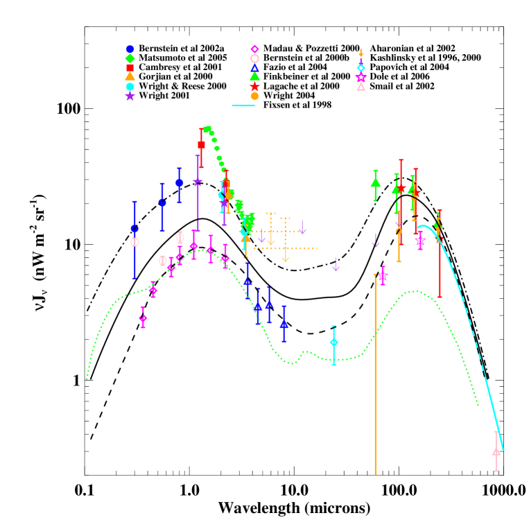
Figure 1: The observed extragalactic background light. Sources for observational points and limits are given in the legend. Filled symbols represent absolute measurements of the background light, while empty symbols represent integrated galaxy counts. The filled circles for the Bernstein et al. (2002a,b) absolute background incorporate the changes in their erratum. We show the analytic fit to the FIR measurement of Fixsen et al. (1998). For the gamma-ray limits of Aharonian et al. (2002) we show squares corresponding to their tentative detections of $\tau=1.5$ at 5.5 TeV for Mkn 501 and $\tau=5.5$ at 4.0 TeV for H1426+428. We convert these limits to effective IR wavelength and background intensities using the approximations of Aharonian (2001). Upper limits from Kashlinsky et al. (1996a, b) and Kashlinsky & Odenwald (2000) use the power spectrum to estimate the total extragalactic contribution. The dashed, solid, and dot-dashed black curves show the traces through this data that are discussed in the text. The dotted curve shows results from the semi-analytic model of Primack et al. (2005).

Integrated galaxy counts in the optical/NIR region were compiled by Madau & Pozzetti (2000), who suggested that the flux had essentially converged. In contrast, Bernstein, Freedman, & Madore (2002b) argued that the isophotal magnitudes used in these estimates failed to capture much of the flux from the faint portions of galaxies, and found substantially higher estimates from an “ensemble photometry” technique, as shown by the open circles in the figure. Fazio et al. (2004) provide integrated galaxy counts in the NIR from Spitzer, which are not as close to convergence as those in the optical.

Direct measurements of the absolute background by Bernstein, Freedman, & Madore (2002a,b) give substantially higher values. These authors attribute the differences in the optical region to two effects: flux missed by normal galaxy count surveys in the outer, diffuse parts of galaxies (partially recovered by the ensemble photometry technique) and high-redshift galaxies that are missed altogether by these surveys owing to their low surface brightness. Direct measurements in the NIR, using the space instruments DIRBE (Cambrésy et al., 2001; Gorjian et al., 2000; Wright & Reese, 2000; Wright, 2001) and IRTS (Matsumoto et al., 2005), mainly give even higher estimates, particularly the latter. The dispersion among these DIRBE points is mainly from different ways of analysing the foregrounds, including different ways of subtracting stars and different models for the zodiacal light. The zodiacal light subtraction is likely the largest source of systematic error in these direct background measurements, especially since the shape of the NIR excess nearly matches that of the zodiacal light (Dwek et al., 2005). It is perhaps encouraging that all of the optical and NIR direct background estimates from different groups give values significantly higher than the direct counts, suggesting that at least part of the excess signal is real. To many authors, the apparently peaked NIR excess suggests a Ly$\alpha$-dominated contribution from Pop III stars before reionisation at $z>10$ (e.g., Santos et al., 2002). However, this model has some major problems stemming from its large energy requirements (Madau & Silk, 2005) and observational constraints on the number of NIR-detected Ly$\alpha$ emitters (Salvaterra & Ferrara, 2006).

Turning to the mid- and far-IR region, we show integrated galaxy counts derived from Spitzer observations at 24 µm (Papovich et al., 2004). We also show the integrated light derived from an analysis at 70 and 160 µm by Dole et al. (2006), who stacked the observed 24 µm sources and integrated the resulting light in these other bands. In both cases, we show only the flux resulting from the observed counts, rather than their extrapolation of the counts to zero flux, which would raise the plotted points by 20–40%. The faint counts in these analyses are heavily dependent on estimating the detection completeness against the background of unresolved sources, and future work on this issue may well result in slightly different faint-end slopes, which would strongly affect the extrapolation.

The absolute background detections in the far-infrared (FIR) region come from the DIRBE and FIRAS experiments on board COBE. For the DIRBE data originally obtained by Hauser et al. (1998), different groups have treated the photometric calibration and foreground subtraction in different ways, leading to multiple results from the same data (Finkbeiner et al., 2000; Lagache et al., 2000; Wright, 2004). At 240 µm  the different results are nearly in agreement, but as the wavelength decreases the scatter among them increases, probably because of the greater complications associated with the higher zodiacal light intensity. These shorter-wavelength points can have a strong effect on the estimated height and width of the FIR peak. We have represented the longer-wavelength FIRAS data by the analytic fit in Fixsen et al. (1998), rather than the noisier raw data.

TeV $\gamma$-ray measurements towards blazars can in principle measure the background via the opacity to 2-photon scattering. In our judgement, these measurements are not yet very reliable; the estimated optical depth is extremely sensitive to the assumed shapes of both the intrinsic TeV source and the background spectrum itself. Hence at this point, we prefer to use direct absolute background detections, even though they are uncertain. However, in the MIR range only loose upper limits exist as the galaxy signal is too low to compete with the zodiacal light (Hauser et al., 1998). We thus show results of optical depth models towards two blazars presented in Aharonian et al. (2002), using the formulae of Aharonian (2001) to convert optical depth to MIR background intensity. These arrows are tentative detections but should probably be treated as upper limits. We note that TeV $\gamma$-ray absorption estimates should be best at constraining sharp, intense features in the background; it would be at least somewhat surprising if the NIR peak shown by the IRTS data is consistent with existing TeV data (Aharonian et al., 2005). To strengthen the case for a lower EBL in the MIR region, we show the results of fluctuation analyses by Kashlinsky et al. (1996a), Kashlinsky et al. (1996b), and Kashlinsky & Odenwald (2000), which attempt to place limits on the galaxy contribution from the power spectrum of the background rather than its absolute intensity.

As mentioned above, and as is apparent in the galaxy counts in Figure 1, the galaxy contribution to the extragalactic background is expected to have two broad humps. A model of the background radiation (Primack et al., 2005) is shown by the dotted line; while this clearly underestimates the background intensity especially in the FIR, it indicates the expected shapes. For our work, we require better estimates of the total intensity. We show three traces through this plot, representing what we consider the minimum (dashed line), maximum (dot-dashed line), and best guess (solid line). These curves are simply constructed to be smooth curves without a particular functional form, but their shapes do reflect global galaxy emission models. The “max” trace uses the background measurements in the optical and NIR and the MIR gamma-ray limits, while the “min” trace follows the lower values implied by the galaxy counts. The “mid” trace adopts a compromise between the higher galaxy counts and the lower range of absolute background estimates. In the FIR, the differences between these curves are unrelated to those in the optical, and mainly reflect the assumed width of the FIR peak. The total background fluxes for these traces are 50, 77, and 129 bgu. If we consider only the optical/NIR portion below 10 µm, we get 22, 36, and 70 bgu, while if we consider only the FIR portion above 10 µm, we get 28, 41, and 59 bgu.

Our EBL estimates range to substantially higher values than the best estimate of $55\pm 20$ bgu determined by Madau & Pozzetti (2000), which was later revised and increased to 60 bgu by Madau et al. (2001). Later estimates, which include 60–93 bgu by Gispert, Lagache, & Puget (2000), 45–170 bgu with a preferred value of 100 by Hauser & Dwek (2001), and $100\pm 20$ bgu by Bernstein, Freedman, & Madore (2002b), are more in line with our estimate. The crucial issues contributing to this uncertainty are not statistical error but systematics like the calibration of the FIR measurements, the zodiacal light subtraction in the optical and NIR background measurements, the treatment of the falloff from the optical and FIR peaks to the MIR region, and simply which data points to include. Illustrating the latter issue, Dole et al. (2006) recently discussed the EBL in the context of their FIR galaxy stacking analysis. They rely on limits from TeV $\gamma$-ray absorption and IR fluctuation analyses to set the upper limits on the flux, whereas we have preferred absolute background detections. The upper and lower boundaries of their allowed region are shown in their Figure 12. Using these traces and adopting a higher-order integration scheme than used in their derivation, we find that the $J_{\it EBL}$ is in the range of 52–77 bgu, spanning approximately the lower half of the allowed range we find here.

Below, we will need to estimate the probability (or likelihood) distribution of $J_{\it EBL}$. It is clear that this distribution is far from Gaussian, as the galaxy counts provide a hard lower limit to the background in certain portions of the spectrum, but the correlated and conflicting data points mean that it is hard to estimate the likelihood function in an objective way. Our approach is to split the wavelength regime in two at 10 µm, since the values in the optical/NIR and FIR are essentially unrelated. In each of these ranges, we take the likelihood to have a constant (top-hat) distribution in log space between our minimum and maximum traces. We then convolve the two distributions together to describe the sum of the flux in the two wavelength regions.

Of course, active galactic nuclei (AGN) also contribute to the background energy. This energy is emitted mainly in a UV/optical peak, a roughly power-law X-ray tail, and an MIR/FIR peak from dust-processed radiation. However, the AGN contribution to $J_{\it EBL}$ appears to be much smaller than that of star-forming galaxies. For example, Hopkins et al. (2006) present a detailed model of the AGN and supermassive black hole populations that fits (partly by construction) quasar luminosity function data over a wide range of wavelengths and redshifts. Their Figure 22b plots the growth of the average black hole mass density with redshift, and we can compute the corresponding contribution to the bolometric background radiation using their assumed radiative efficiency of $\epsilon_{r}=0.1$ (essentially using the argument of Soltan, 1982). We obtain $J_{AGN}=1.9^{+1.5}_{-0.8}$ bgu, where the uncertainty is scaled from the uncertainty in their prediction of the $z=0$ black hole mass density, $\rho_{BH}=2.9^{+2.3}_{-1.9}\times 10^{5}\,M_{\sun}\,\mbox{Mpc}^{-3}$. Note that this argument does not assume that the Hopkins et al. (2006) scenario is physically correct, just that it fits the observed luminosity functions within their uncertainties and, therefore, reproduces the observed total emission. Furthermore, the model’s predicted $\rho_{BH}$ agrees with observational estimates (e.g., Aller & Richstone 2002; Marconi et al. 2004), and there is no room for a large amount of additional AGN contribution to $J_{\it EBL}$ without overproducing these estimates. A significant fraction of this bolometric AGN background appears in X-ray wavelengths and therefore does not add to the UV/Optical/IR background considered here. As another check of $J_{AGN}$, the model of Silva et al. (2004), which is based on AGN counts in X-ray and IR bands and has recently received further observational support from Treister et al. (2006), implies the AGN contribution in all wavebands is $\sim\!1.4$ bgu, and that in the UV/Optical/IR background it is 1.1 bgu (Silva, private communication). We conclude that the AGN contribution cannot be much larger than 4%, and is probably somewhat lower, and we ignore it henceforth.

The issue of whether or not the integrated galaxy counts match the total EBL has implications for this paper beyond just a change in the total bolometric background. If flux from sources besides normal galaxies are truly required to explain the extragalactic light, and the source cannot be identified, then there is not necessarily a relationship between the total EBL and the energetic output from stars! However, the need for additional sources of energy is not at all clear at present. The systematic uncertainties, particularly in the galaxy photometry and zodiacal light subtraction, suggests that a curve splitting the difference between the raw counts and measured total background (as in our “mid” model) represents the most conservative assumption. Also, if the excess over total normal-galaxy counts should turn out to be real, a candidate for explaining the excess in the NIR, where it appears most significant, exists in the form of Population III stars. According to models of these sources, they would contribute almost all of their energy in the wavelength range 1–5 µm, leaving the background at other wavelengths essentially unchanged. This would imply that our lower limits on the optical/NIR background (which ignore the NIR excess) and our traces of the FIR background are still valid.

3.2 Star Formation History

The cosmic star formation history is related to both the EBL and the stellar mass observable today. Observational estimates of the SFH at various redshifts are shown in Figure 2. This plot uses a combination of IR (stars), UV continuum (filled symbols), and emission-line surveys (open symbols). We have tried to use the deepest and broadest surveys within each type, so some of the pioneering SFH surveys have been omitted. The plot also shows the sub-mm points from Barger, Cowie, & Richards (2000, crosses), including both their actual source detections and their extrapolation to account for the entire sub-mm background, as well as the estimate of the total SFR in the damped Ly$\alpha$ population from Wolfe et al. (2003). We do not use the sub-mm or damped Ly$\alpha$ points in the fit. We omit estimates from radio and X-ray surveys, because the energetic calibrators are even more uncertain than those in the UV and FIR.

For the UV continuum measurements, we have combined results at 2800 Å from Connolly et al. (1997) and Wolf et al. (2003), and results at 1500–1700 Å from Steidel et al. (1999), Gabasch et al. (2004), Giavalisco et al. (2004), Schiminovich et al. (2005), Sawicki & Thompson (2005), and Bouwens et al. (2006). For the IR measurements we include the local IRAS survey of Yun, Reddy, & Condon (2001) and the Spitzer 24 µm survey of Pérez-González et al. (2005). For emission-line measurements, we restrict ourselves to H$\alpha$ because metal lines like [O II] might be biased by evolution of the metallicity and we use the values listed in Hopkins (2004) from the surveys of Gallego et al. (1995), Tresse & Maddox (1998), Yan et al. (1999), Sullivan et al. (2000), Hopkins et al. (2000), Tresse et al. (2002), and Pérez-González et al. (2003). We use only the H$\alpha$ estimate from Sullivan et al. (2000) because the UV continuum magnitudes used there have been brought into question by more recent results from GALEX (Schiminovich et al., 2005).

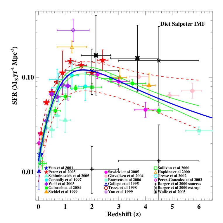
Figure 2: Star formation rate per unit comoving volume as a function of redshift as derived from observations. The observational points, which are labelled by source, have been rescaled to our chosen “737” cosmology, and to a common set of luminosity and completeness calibrations using the “diet” Salpeter IMF as discussed in the text. We use uniform dust correction factors for the optical and UV points (see the text for details). The thick solid line is our best fit to the data. The thin solid and thin dashed curves indicate the $1\sigma$ envelope of the fits in our standard and “random-calibration-error” samples of fits, respectively.

We convert the calibration factors used by the various authors to the uniform values given in Table 2, using a diet Salpeter IMF with $10^{8}\,\mbox{yr}$ bursts. We have converted all the star formation rate densities to our standard cosmology, since they scale with the Hubble constant, $H(z)=\dot{a}/a$. This cosmology dependence factors out when integrating over time to get $\rho_{\star{\it form}}$, although $\rho_{\star{\it rem}}$ can shift by a percent or so owing to the dependence of $f_{\it mass}$ on cosmic timescales.

The UV surveys, in general, do not probe deep enough in luminosity to make the integrated star formation rate converge. Most authors calculate the total by fitting a Schechter form to the luminosity function and extrapolating either to zero flux or to an arbitrarily chosen lower limit. For consistency, we adjust these reported values to a uniform extrapolation down to $0.1L_{\ast}$ where $L_{\ast}$ is the Schechter turnover luminosity reported for each survey. Extrapolating down to $0.01L_{\ast}$ instead would cause the values to increase by 20–45%. In many cases ours is the approach used by the original authors; in the others the change in the extrapolation has a rather minor effect compared to the scatter between surveys. In contrast to the UV, the H$\alpha$ surveys are deep enough that they require no extrapolation.

To make the UV continuum extinction corrections reasonably uniform, we use the correction formula of Calzetti (1999), assuming the mean value of $E(B-V)=0.15$ given by Steidel et al. (1999). This yields correction factors of 3.1 and 4.7 at 2800 and 1500 Å, respectively. The one exception is the highest-redshift point of Bouwens et al. (2006), for which we have used the correction factor of 2.0 estimated by the authors from the mean UV slope in the sample. At lower redshifts, some authors have used this UV slope correction method to obtain higher extinction values than we have assumed (e.g., a factor 7 in both Schiminovich et al., 2005 and Giavalisco et al., 2004).

For the H$\alpha$ measurements, we used the uniform luminosity-dependent extinction calibration of Hopkins (2004). The two FIR surveys are not “transmission-corrected” for the amount of UV light that leaks out directly from the galaxies, but this is likely a significant fraction. In fact, at low redshifts the UV and FIR luminosity estimates are roughly equal (Martin et al., 2005). We have crudely assumed a correction factor of 2.0 for $z<1$ and 1.2 for $z\geq 1$. All of these extinction and transmission estimates are clearly highly uncertain, and among the largest of the calibration errors in the observed SFH.

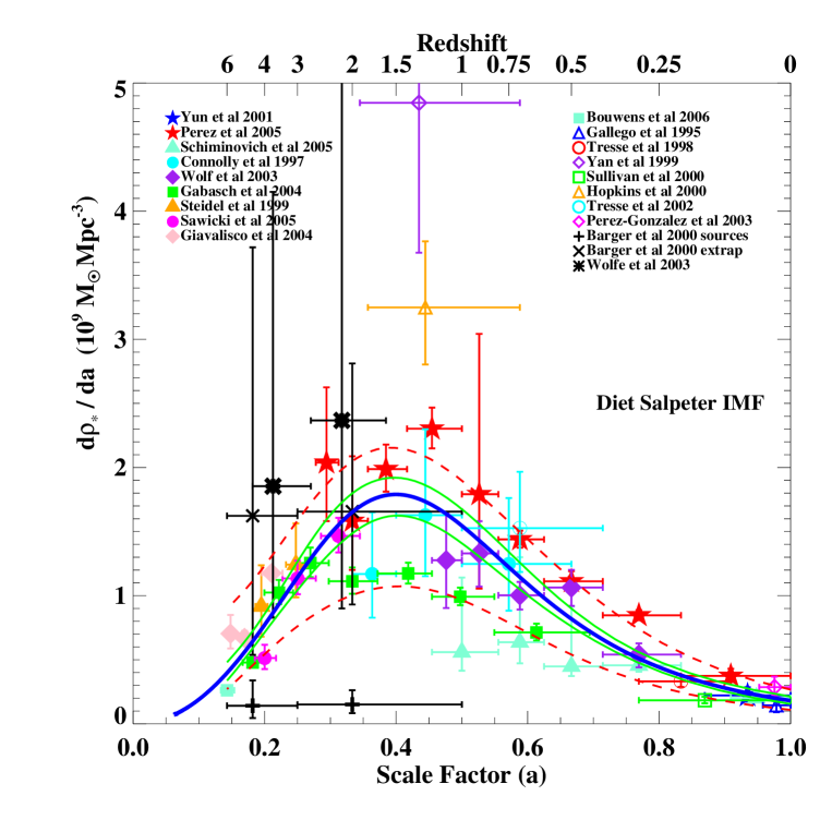
Figure 3: Star formation rate per unit scale factor versus scale factor. This is similar to Figure 2 but with rescaled axes. The vertical axis here is the derivative of the mass of stars formed with respect to the scale factor, $d\rho_{\star{\it form}}/da=(1+z)\dot{\rho}_{\star{\it form}}/H(z)$. In this form the data points are independent of cosmology, and the total star formation is the area under the data points. One can easily see the relative importance of different redshift ranges.

In Figure 3 we replot the SFH such that one can easily integrate under the data points by eye to get the total mass of stars formed: $d{\rho_{\star}}/da$ versus scale factor $a$. This plot makes it straightforward to see the relative importance of star formation at different epochs in determining the stellar content today. Clearly, most of the uncertainty in the total stars formed comes from the redshift range $1\la z\la 3$. While there is still a surprisingly high dispersion in low-redshift ($z<0.5$) estimates of the star formation rate, the figure shows it is of little significance to the total stellar mass.

In these plots, it is unclear how well individual observations capture the whole census of star formation at any redshift. At high redshift, several populations of sources have been suggested as major contributors to the total star formation, including diffuse red galaxies (Webb et al., 2006), damped Ly$\alpha$ absorbers (Wolfe et al., 2003), Ly$\alpha$ emitters (e.g., Tapken al., 2006), and sub-mm galaxies (Barger, Cowie, & Richards, 2000; Chapman et al., 2005). For all of these categories, the extent of overlap with the Lyman-break galaxies, for example, is still unclear. The mere presence of one population in a second population may not suffice; for example, the large star formation rates found for the bright sub-mm sources are essentially invisible to the SFR estimates made in the UV (Chapman et al., 2005). Hence, it is possible that the SFR estimates obtained from these different populations should be added together, rather than plotted together as different measures of the same quantity. This could raise the true SFR by perhaps a factor of 2 above the individual points.

To compare this large spread of data points to other measures of star formation, it is useful to obtain analytic fits to the star formation history. Here we introduce a new parametric form: we set

$$\rho_{\star{\it form}}(z)=\rho_{0}/(1+p_{1}a^{-p_{2}})^{p_{3}}$$ (5)

where $a=1/(1+z)$ is the scale factor. Then

$$\dot{\rho}_{\star{\it form}}=\frac{p_{1}\,p_{2}\,p_{3}\,\rho_{0}\,a^{-p_{2}}}{(1+p_{1}a^{-p_{2}})^{p_{3}+1}}H(z)\;.$$ (6)

This functional form has the advantages of easily relating $\dot{\rho}_{\star{\it form}}$ and $\rho_{\star{\it form}}$, and of making the dependence on cosmology explicit. This parameterisation is a particularly natural choice for Figure 3, since $d\dot{\rho}_{\star{\it form}}/da=\dot{\rho}_{\star{\it form}}/\left[aH(z)\right]$ is a simple analytic function.

We use a $\chi^{2}$ technique to fit the data. The reported errors for the different points vary widely, depending mostly on sample size; for those with the smallest errors, the systematic errors in calibration and extrapolation probably swamp the formal errors, which are derived from Poisson statistics alone. Rather than trying to revise the error derivation of every literature source, we simply add an error of 0.1 dex in quadrature to the errors on the points before fitting the data, which restores the best-fit $\chi^{2}$ to an acceptable value of 44 for 42 degrees of freedom. The best-fit parameters are $\rho_{0}=9.0\times 10^{8}\,M_{\sun}\,\mbox{Mpc}^{-3}$, $p_{1}=0.075$, $p_{2}=3.7$, and $p_{3}=0.84$.

To test for a possible dependence of our results on the parametric form, we also use the form of Cole et al. (2001):

$$\dot{\rho}_{\star{\it form}}=\frac{(a+bz)h}{1+(z/c)^{d}}\;.$$ (7)

Here the dependence on the present-day Hubble constant is factored out, although not that of the other cosmological parameters. This form has the same number of free parameters as the previous one and has been widely used in the literature. Fitting the data as before, our best fit is $a=0.0103\,M_{\sun}\,\mbox{yr}^{-1}\,\mbox{Mpc}^{-3}$, $b=0.088\,M_{\sun}\,\mbox{yr}^{-1}\,\mbox{Mpc}^{-3}$, $c=2.4$, and $d=2.8$ with $\chi^{2}=44.7$ for 42 degrees of freedom. The curves produced by these two parameterisations are nearly indistinguishable from each other.

We want to probe not just the mean value but the full allowed range of star formation histories. To do this, we construct an ensemble of parametric fits, using a Monte Carlo Markov chain and assuming uniform priors on the logarithm of the parameters. The ensemble evenly samples the probability distribution of the fits. We can then estimate the allowed ranges of $\dot{\rho}_{\star{\it form}}(z)$ at any $z$ from the ensemble of fits. (A simple grid search in parameter space was also tried, and produced essentially identical results.) The typical formal $1\sigma$ error in $\dot{\rho}_{\star{\it form}}$ is only 10–15% for $z<5$, as shown in Figure 2. The widths of these envelopes are quite similar to those of Hopkins & Beacom (2006), despite the different data sample, sampling procedure, and parametric form.

However, it is likely that this procedure underestimates the true errors in the determination of $\dot{\rho}_{\star{\it form}}$. For example, the best fit in Hopkins & Beacom (2006) appears to lie well above our error envelope for $2<z<4$, owing to a different selection of data points, different assumptions about extinction, and a larger extrapolation of the luminosity function. While the large number of data points with small Poisson errors result in a small formal error in our fit, this masks the larger uncertainties in calibrating $\dot{\rho}_{\star{\it form}}$, which applies equally to all the points. Even with a fixed IMF, there are substantial uncertainties in the mean opacity at a given redshift and in the calibration of luminosities owing to the uncertain star formation histories of individual galaxies (see §2). The systematic errors at different redshifts are undoubtedly correlated, although there is speculation that the mean opacities at $z\sim 0$, $z\sim 2$, and $z>4$ are substantially different from one another.

Therefore, we produce an alternate grid of fits in which we randomly and smoothly adjust the $\dot{\rho}_{\star{\it form}}$ data values as a function of redshift. We first define three random variables $A(0)$, $A(1.5)$, and $A(5)$, and set each to have normal distributions of dispersion $\sigma_{A}=0.5$. We then multiply the data values and associated errors by $e^{A(z)}$, where $A(z)$ is the quadratic function in $z$ through the three points $A(0)$, $A(1.5)$, and $A(5)$, and repeat the previous Monte Carlo sampling procedure. Not surprisingly, this procedure results in a much broader range of acceptable parameters, and a correspondingly wider envelope of $\dot{\rho}_{\star{\it form}}$ at any given redshift, as shown in Figure 2. Given the large uncertainties discussed above, $\sigma_{A}=0.5$ is probably reasonable. The 1-$\sigma$ dispersion in the SFH is then about 50% or 0.2 dex for $z<4$.

3.3 Stellar mass and NIR luminosity density

The third observable we need to consider is the stellar mass density. We are primarily concerned with the value of this quantity today but we shall also consider the evolution of stellar mass with cosmic time. NIR light is a useful proxy for stellar mass, since plausible values of $M/L$ vary only by a factor of a few and this variation can be accounted for using simple colour-based estimates (Bell & de Jong, 2001). Like the star formation rate, the stellar mass and luminosity densities determined from observations are proportional to $H(z)$, and we have translated the measurements below to our assumed cosmology.

We shall use five studies of NIR light and stellar mass at low redshifts. All the studies in the $J$ and $K$ bands use 2MASS magnitudes, combined with various redshift surveys. The results of these local surveys are given in Table 3.

Cole et al. (2001) use the 2dF redshift survey in the southern sky, combined with the second incremental release of 2MASS, to obtain $J$, $K$, and stellar mass densities. They use Kron aperture magnitudes, calibrating the preliminary 2MASS catalogue against deeper $K$-band data and correcting their estimate of $\rho_{\star{\it rem}}$ for missing light outside the Kron radius. However, they do not similarly correct their reported estimate of $\rho_{K}$, so we have scaled up their Kron magnitude based estimate by 0.11 magnitudes to get the total light. To determine the stellar mass density they estimate the mass-to-light ratio galaxy by galaxy using the observed optical-to-near-infrared colours to constrain the effects of the star formation history and metallicity in each galaxy. They check for the effect of missing low-surface-brightness galaxies in the relatively shallow 2MASS sample and conclude that that any such effect should be small.

Bell et al. (2003) use the Sloan Digital Sky Survey (SDSS) Early Data Release in the northern sky, combined with the final 2MASS survey, to obtain $K$-band and stellar mass densities. They also use Kron magnitudes but scale up the luminosities of the early-type galaxies by 0.1 mag to account for light outside the Kron aperture. They estimate their $M/L$ ratios by means of optical galaxy colours; they neglect the effect of extinction entirely since it affects the mass estimate both through the flux and the colour, and these should nearly cancel out (Bell & de Jong, 2001). They go on to suggest that the 2MASS catalogue may miss some low-surface-brightness galaxies and estimate the magnitude of this effect in three ways. First, estimating the $K$-band light density using the $r$-band luminosity density, which should be complete at these magnitudes, and the global $r-K$ colour for their sample, they find $\rho_{K}$ increases by 12%. Second, using their $g$-band-selected galaxy sample and synthesising the $K$ magnitudes of galaxies missing from the $K$-band sample from their optical magnitudes, they find $\rho_{K}$ increases by as much as 30%. This $g$-band estimate might be biased since when they obtain the stellar mass density using the complete $g$-band optical sample it is only 4% higher than their estimate using their uncorrected $K$-band magnitude limited sample. Hence, in this paper we use their direct estimates of mass and light from the $K$-band sample.

Panter et al. (2004) analyse galaxy spectra in the first data release of the SDSS at 20 Å resolution. They obtain total fluxes by normalising the spectroscopic fibre magnitudes to photometric $R$-band Petrosian magnitudes. (We note that Petrosian magnitudes may underestimate the flux from early-type galaxies by about 20%, although they are probably very accurate for disk galaxies (Strauss et al., 2002; Graham & Driver, 2005). They then fit galaxy models to compressed versions of the spectra to obtain the local stellar mass density.

Eke et al. (2005) use an updated version of the 2dF redshift survey together with the updated 2MASS catalogue to produce a larger sample than Cole et al. (2001), obtaining $J$-band, $K$-band, and stellar mass densities. Eke et al. calculate galactic stellar masses using star formation histories that include bursts. When tested against mock galaxy catalogues, this reduces the average stellar masses by 20–30%. Whether or not this results in a smaller bias, however, depends on the validity of the star formation histories in the mock catalogues. Eke et al. show that the mass function obtained from their optically-selected sample differs systematically from that obtained using the $J$-band selected sample, which they cite as possible support for the bias against low-surface-brightness galaxies found by Bell et al. (2003). However, the difference starts starts to occur where the computed biases in the optically-based and NIR-based mass estimates from the mock catalogues start to diverge, making its significance unclear.

Finally, Jones et al. (2006) combine 2MASS with a preliminary catalogue from the wide-angle 6dF redshift survey and determine $J$-band and $K$-band luminosity densities. They use “total” (extrapolated) 2MASS magnitudes to obtain the galaxy luminosities. Since they do not explicitly state a error estimate, we read it off their Figure 15. They also argue that their sample is robust to surface brightness effects on the total luminosity density.

Table 3: Local Stellar Mass and Light (for diet Salpeter IMF)

$\rho_{z}^{a}$	$1.93\pm 0.20$	Bell et al. (2003)
$\rho_{J}^{b}$	$2.11\pm 0.31$	Cole et al. (2001)
	$2.43\pm 0.08$	Eke et al. (2005)
	$2.22\pm 0.15$	Jones et al. (2006)
weighted avg	$2.37\pm 0.36$	(assuming 15% systematic error)
$\rho_{K}^{c}$	$4.24\pm 0.64$	Cole et al. (2001)
	$4.08\pm 0.09$	Bell et al. (2003)
	$4.66\pm 0.15$	Eke et al. (2005)
	$4.30\pm 0.37$	Jones et al. (2006)
weighted avg	$4.24\pm 0.64$	(assuming 15% systematic error)
$\rho_{\star{\it rem}}$	$3.94\pm 0.58$	Cole et al. (2001)
	$3.71\pm 0.07$	Bell et al. (2003)
	$3.26\pm 0.11$	Panter et al. (2004)
	$3.08\pm 0.14$	Eke et al. (2005)
unweighted avg	$3.50\pm 0.70$	(assuming 25% systematic error)
aUsing $M_{\sun(z)}=4.53$ (Bell et al., 2003)
bUsing $M_{\sun(J)}=3.33$ (Worthey, 1994)
cUsing $M_{\sun(K)}=3.70$ (Worthey, 1994)

For our purposes we must compare the different estimates using the same assumptions. First, we compute the luminosity densities for each estimate using the same value for the sun’s absolute magnitude in each band, obtaining the densities in Table 3. Since the luminosity densities were computed in a similar way by each group, we first average the luminosity density estimates after weighting by the inverse of its variance, and take the harmonic sum of the variances to get the statistical error. We then add an overall systematic error of 15% (cf. Bell et al., 2003), which dominates the error in all cases.

To compute the stellar mass densities, we first convert all the mass estimates to a diet Salpeter IMF, assuming 0.7 times as much mass as for a Salpeter IMF and 1.74 times as much mass as for a Kennicutt IMF. We then take a straight average of the four estimates, since for each data point the systematic error outweighs the statistical error and we do not know which approach is best. We then assign an overall systematic error of $20\%$ (cf. Bell et al., 2003), which may be reasonable as the varied approaches here yield a dispersion of only 10%. Our final estimate of $(3.50\pm 0.70)\times 10^{8}\,M_{\sun}\,\mbox{Mpc}^{-3}$ for a diet Salpeter IMF implies $\Omega_{\star}h=(1.8\pm 0.4)\times 10^{-3}$ and $F_{\star}=\Omega_{\star}/\Omega_{b}=0.063\pm 0.016$. This estimate is lower by more than a factor of two than the earlier best estimate of Fukugita, Hogan, & Peebles (1998) using $B$-band data, once we account for the different IMF.

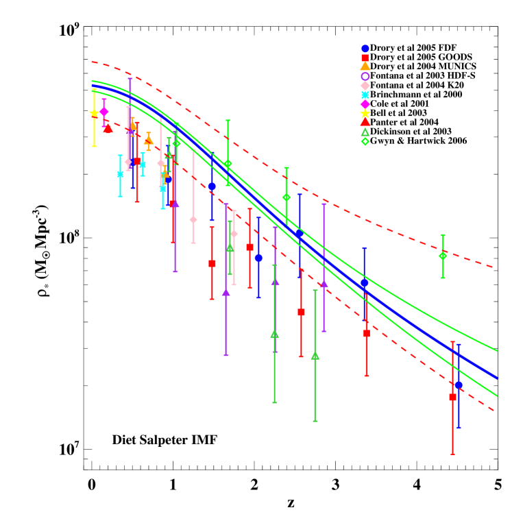
Figure 4: Stellar mass as a function of $z$ scaled to a diet Salpeter IMF (at $z=0$ this scaling factor is 0.70 and it slowly increases to 0.74 at $z=5$). Sources of the data points are as indicated. The heavy solid line shows the result of integrating our best fit through Figure 3, including the appropriate recycling factor. The light solid and dashed lines show the $1\sigma$ boundaries of our “normal” and “randomly-recalibrated” ensembles of fits, respectively.

Recently, attempts have been made to estimate the stellar density at higher redshift as well, based on faint galaxy catalogues with multi-band photometry. This is even more difficult than estimating the high-redshift star formation rate density, both because surface brightness dimming interferes more with regions of less intense emission and because their estimates must be based on the rest-frame optical light rather than rest $K$-band, which increases the uncertainty in the mass. In Figure 4 we show a number of observational estimates for $\rho_{\star}(z)$. Most of these points were originally derived for a Salpeter IMF. We rescale them to a diet Salpeter IMF using the ratio of population masses calculated from our best-fit star formation history; we find this to be a factor of 0.70–0.74. The different studies use a variety of assumptions about stellar populations, extinction, and methods for calculating the mean $M/L$ ratios. In most cases we plot the error bars given by the authors, which are usually purely from Poisson statistics. However, for Dickinson et al. (2003) we plot error bars based on their dominant uncertainty, modelling the stellar population. The largest estimates of $\rho_{\star}$ at high $z$ are from Gwyn & Hartwick (2005) but it is not clear whether or not these higher estimates arise from their use of deeper UDF data.

The systematic errors in the measurement of the total stellar mass and light deserve some further discussion. Extrapolation beyond the faint or bright end of the observed luminosity function is not a significant factor in the surveys of the local universe discussed above (Cole et al., 2001; Panter et al., 2004). These surveys make corrections for flux outside the apertures and these apertures are quite wide to begin with, e.g. $\sim\!20$–$40\,\mbox{kpc}$ in radius for a massive disk galaxy, but these corrections do not take into account the power-law halos that commonly surround galaxies (Mouhcine et al., 2005; Guhathakurta et al., 2005). However, using the mass fraction and density profile suggested for M31 by Guhathakurta et al. (2005), it appears the extra correction would only amount to 2%.

Free stars not clearly bound to any single galaxy could be another source of error. Observations of red stars (Durrell et al., 2002) and planetary nebulae (Okamura et al., 2002) suggest free stars make up 10–20% of all the stars in the Virgo cluster. However, as clusters contain only about 2% of all the stars in the universe (Eke et al., 2005), it by itself is not a significant correction. In simulations of galaxy formation presented in a related paper (Fardal et al. 2006, in prep), free stars are found preferentially in and around galaxy clusters owing to the intense tidal interactions present there, so once again the global fraction of free stars should be well below that estimated for Virgo and be negligible for our purposes here.

Systematic effects from low-surface-brightness galaxies unrepresented in the 2MASS catalogue are potentially a larger problem; the various estimates of their significance in the discussion above range from 0 to 30%. We will assume that this is not a significant bias, but the reader should keep in mind that the true luminosity and mass densities could potentially be raised by as much as $\sim\!30\%$ by this effect.

Finally, the calculation of $M/L$ ratios of individual galaxies, something which is required in all these papers, is uncertain owing to many factors including uncertainties in: the metallicity, the star formation history, the extinction, the stellar tracks, and the population synthesis methods themselves. The derived distribution of the metallicity may also have a substantial effect, particularly on the $K$-band light from RGB and AGB stars. The latter stars are quite difficult to simulate, and regardless of the metallicity they are a major source of error in the stellar population calculation. To indicate the dispersion, the different methods of Cole et al. (2001), Bell et al. (2003), and Eke et al. (2005) give $M/L_{K}$ estimates of 0.88, 0.92, and 0.62 respectively, and our combined sample gives a net result of 0.83. This range of estimates is in accord with the $\sim\!25\%$ systematic errors in $M/L$ (for a fixed IMF) estimated by Bell et al. (2003). Observationally testing the distributions of star formation, extinction, and metallicity derived in local surveys will help control the systematic errors involved in calculating the stellar mass.

4 COMPARISON OF STAR FORMATION MEASURES

We now turn to the central question of this paper: are the direct estimates of the cosmic star formation history, the measured bolometric background intensity, and the local density of $K$-band light mutually compatible, given the assumption of a universal IMF with a Salpeter-like shape above $0.9\,M_{\sun}$? The curves in Figure 4 show the stellar mass density as a function of redshift computed from the star formation history traces shown by the corresponding curves in Figures 2 and 3. The lowest curve, which reduces the standard normalisation of the SFR estimates by about a factor of two (see §3.2), roughly follows the median of the data points, while the other curves are systematically higher than the data. We have included the slight variation with redshift of the recycled mass fraction in this calculation. Although many factors could contribute to systematic errors, it is of particular note that a substantial amount of stellar mass could be missing from the high-redshift observational surveys owing to surface brightness effects. The tension between the SFR and stellar mass density estimates provides circumstantial evidence for such effects. If lower surface brightness galaxies are indeed missed in the high redshift counts, it would help resolve the discrepancy between the absolute background light estimates and the integrated count estimates, suggesting that the higher, absolute estimates are more accurate.

For the remainder of this section, we will focus on $z=0$, since the observational estimates of the stellar mass density are more secure in the local universe and, even more important, we can bring in the bolometric background (which is only measured at $z=0$) as an additional observational constraint. We will mainly focus on the local $K$-band light density $\rho_{K}$ rather than the stellar mass density $\rho_{\star{\it rem}}$, since it is the directly observable quantity. We integrate each SFH fit to obtain the predicted final stellar mass $\rho_{\star{\it rem}}$ and $K$-band luminosity density $\rho_{K}$ as in Equation 1, and the EBL, $J_{\it EBL}$, as in Equation 3. (The integrations cover the range $z\leq 15$ in each case.) We include the extinction correction $e^{-\tau_{K}}$ discussed in §2 to make $\rho_{K}$ an observed luminosity density.

According to our direct SFR fits (assuming no calibration error), the mean $\rho_{\star{\it rem}}=(5.3\pm 0.3)\times 10^{8}\,M_{\sun}\,\mbox{Mpc}^{-3}$, or $F_{\star}=0.095\pm 0.005$. The corresponding predicted extinction-corrected $\rho_{K}=(6.9\pm 0.4)\times 10^{8}\,L_{\sun K}\,\mbox{Mpc}^{-3}$. (We obtain the same results whether we use our new parametric form in Equation 6 or that of Cole et al. (2001) in Equation 7.) Including an extra calibration error with $\sigma_{A}=0.5$, we obtain $\rho_{K}=(6.9\pm 2.2)\times 10^{8}\,L_{\sun K}\,\mbox{Mpc}^{-3}$. Our adopted value for the observed density is $(4.2\pm 0.6)\times 10^{8}\,L_{\sun K}\,\mbox{Mpc}^{-3}$. Thus the integrated SFH should produce more mass and light than that directly observed, by a factor of 1.5 if we use the quoted mass estimates, or by a factor 1.6 if we use the $K$-band luminosity density. The probability of agreement is $<2\%$ without random calibration errors, but rises to 10% and 32% for random calibration error of $\sigma_{A}=0.2$ and 0.5 respectively. Thus, while the offset could indicate that local surveys miss significant amounts of stars, or that some other assumption (such as our IMF) may be wrong, calibration uncertainty in the SFH seems a sufficient explanation. For example, the curve could be made to match the plots by changing the estimates of the UV extinction. Our best SFR fits imply $M/L_{K}=0.71e^{\tau_{K}}=0.77$, which is within the range of values found by Cole et al. (2001), Bell et al. (2003), and Eke et al. (2005).

The appearance of a discrepancy is found by other authors as well, although a number of authors apparently simply scale the integrated SFH to match the $z=0$ stellar mass, without mentioning the scaling factor! Our integrations of $\rho_{\star{\it rem}}$ are in reasonable agreement with the results of Hopkins & Beacom (2006), who found about a 10% uncertainty in the integrated stellar mass from their star formation fits and a value exceeding that expected from direct observations by nearly a factor of 2 (for comparisons using the same IMF). The discrepancy implied by their final mass is even larger than in our case, because their much larger SFR in the range $2<z<4$ contributes a significant amount of mass.

However, we can also include the EBL in the comparisons. Our adopted allowed range of $J_{\it EBL}$ is 50 to 129 bgu, with a most likely value of 77 bgu. Our derived value from the SFH fits is $(63\pm 4)$ bgu without including random calibration error, and $(62\pm 20)$ bgu with $\sigma_{A}=0.5$.

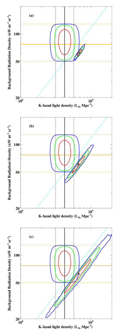
Figure 5: The combined range of $K$-band light and EBL allowed by the range of SFHs. In each panel, the horizontal lines denote the minimum, best guess, and maximum background intensities. The vertical lines denote the best fit and $2\sigma$ error bars on the $K$-band luminosity density. The vertically extended rounded contours show the joint 67%, 95%, and 99.8% joint confidence intervals on these two observed parameters. The diagonally extended contours show the relation of the two quantities in the ensemble of SFH fits, for the following assumptions: (a) No freedom in SFR calibration. (b) Freedom of $\sigma_{A}=0.2$ in SFR calibration (see explanation in text). (c) Freedom of $\sigma_{A}=0.5$ in SFR calibration.

After allowing for fairly large systematic uncertainties, it appears that the estimated cosmic star formation history can be made consistent, individually, with measurements of the local $K$-band light density and the bolometric background intensity. One might, therefore, be tempted to conclude that these three probes of the cosmic star formation are mutually consistent. Figure 5 shows that this is not the case. In the upper left panel, we show acceptable fits in the space of $\rho_{K}$ vs. $J_{\it EBL}$, assuming no systematic errors in the calibration of the SFRs. The vertical lines represent the mean and $2\sigma$ errors in the local $K$-band luminosity density from the combined observations, as discussed in § 3.3. The horizontal lines represent the three values of the background derived in § 3.1. The rounded, vertically extended contours represent joint confidence intervals for these two parameters. We construct these by multiplying the probability distributions of the two parameters together, and finding the contours that enclose 65%, 95%, and 99.8% of the probability. The “squashed” appearance of the contours comes from the non-Gaussian probability distribution of the background light (see §3.1 for an explanation of how we estimate its distribution).

The diagonal contours in panel (a) depict the 65%, 95%, and 99% 2-dimensional confidence regions derived from the ensemble of star formation histories. These contours form a narrow band. If we consider only one dimension, our computed values of $J_{\it EBL}$ are in reasonable agreement with observations, while the stellar mass is rather high as mentioned before. The main point, however, is that the two sets of contours barely overlap; one needs to go out to the $3\sigma$ contours to find agreement. We obtain essentially identical results if we use the Cole et al. (2001) parametric form for the star formation history instead of the form in Equation 6.

The remaining two panels show the results for samples with increasing levels of assumed systematic error in the overall calibration of the SFRs, i.e. a random dispersion in the calibration of $\dot{\rho}_{\star{\it form}}$. This greatly expands the allowed joint confidence region of $K$-band light and EBL so that, as we just discussed, the former is no longer inconsistent with the observations. However, the confidence region still forms an extremely narrow band, which overlaps the observational contours at only the 2 or $3\sigma$ level. Even with this increased freedom, one can find SFR histories that agree well with either the observed $K$ light or the observed bolometric background, but not with both quantities simultaneously.

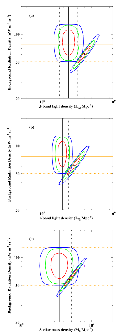
Figure 6: The contours of EBL vs. (a) $J$-band stellar light density, (b) $z$-band stellar light density, and (c) stellar mass density allowed by the range of SFHs. Except for substituting these quantities for $K$-band light, the plots are the same as in the previous figure. In panel (c), the asterisk shows the estimated relation of stellar mass and EBL from Madau et al. (2001), rescaled to our IMF, and the cross shows the result from the simulation of Nagamine et al. (2000) (see text for details).

We consider other proxies for the stellar mass as well. Plotting $J_{\it EBL}$ versus $\rho_{J}$ (instead of $\rho_{K}$) in Figure 6, we see that the $2\sigma$ contours still do not overlap. If instead we use the SDSS $z$-band density, $\rho_{z}$, the contours still do not significantly overlap. The slightly better agreement in $z$-band might suggest that there may indeed be a small bias in the 2MASS surveys owing to missing low surface brightness galaxies. However, our extinction estimates become increasingly suspect as we go to these shorter wavelengths. Finally, we plot the contours of stellar mass itself. With the larger observational uncertainties in this quantity, the disagreement is now at less than the $2\sigma$ level, though the impression remains that either the observed background is too high or the observed mass too low. We regard the $K$-band plots as more fundamental, since they plot a directly observed quantity and one that is tied as closely as possible to the dominant stellar mass range.

In essence, we find that the bolometric background is too bright relative to the present day $K$-band light density, given a Salpeter-like IMF and the shape of the SFH implied by our fits to the observations. Changes to the normalisation of the SFH move predictions along the diagonal in Figures 5 and 6 and, therefore, do nothing to resolve this discrepancy. Our $\sigma_{A}=0.5$ models allow substantial variations in the SFH shape as well as normalisation, but these have limited power to solve the problem. The ratio between the background production function $S_{\it EBL}(z)$ and the $K$-band luminosity $\rho_{K}(z)$ has a maximum at $z\approx 1$ and falls off slowly at higher and lower redshifts. Hence, by the mean value theorem, the ratio between the EBL and the emitted $K$-band luminosity density cannot be larger than

$$\max\left(\frac{J_{\it EBL}(z)}{\rho_{K}(z)}\right) = \frac{c}{4\pi\,e^{-\tau_{K}}}\max\left(\frac{S_{\it EBL}(z)}{l_{K}(z)}\right)$$

$$= 1.21\times 10^{-7}\mbox{bgu}[L_{\sun K}\,\,\mbox{Mpc}^{-3}]^{-1}\;.$$

for a Salpeter or diet Salpeter IMF, including the extinction correction. We plot the maximum ratio as the diagonal dotted line in Figure 5. Because much of the star formation in our calculations takes place at $z\sim 1$, the predicted ratio for our best-fit SFH, $9.0\times 10^{-8}\mbox{bgu}[L_{\sun K}\,\,\mbox{Mpc}^{-3}]^{-1}$, is already 75% of this upper limit, so even a $\delta$-function SFH at $z=1$ can produce only a modest increase. The ratio of our middle trace EBL to our best estimate $\rho_{K}$ is $1.8\times 10^{-7}\mbox{bgu}[L_{\sun K}\,\,\mbox{Mpc}^{-3}]^{-1}$. Getting down to $1.0\times 10^{-7}\mbox{bgu}[L_{\sun K}\,\,\mbox{Mpc}^{-3}]^{-1}$ requires taking our minimal estimate of 50 bgu for $J_{\it EBL}$ (the lower trace in Figure 1) and increasing our averaged value of $\rho_{K}=4.2\times 10^{8}L_{\sun K}\,\,\mbox{Mpc}^{-3}$ by 15%.

With our best SFH fit, 50% of the background is produced in stars that form at $z<1.0$, and the central 80% comes from the stars that form in the redshift range $0.27<z<2.6$. This can be compared with the present-day stellar mass, for which 50% comes from $z<1.2$, and the central 80% comes from the redshift range $0.33<z<3.2$. For the $K$-band luminosity density, 50% comes from stars formed at $z<0.9$, and the central 80% comes from the redshift range $0.1<z<2.7$. Therefore, the EBL principally comes from stars formed at the same redshifts as those that dominate the current mass or $K$-band light, which explains why the correlation is so tight. The background energy is emitted at still lower redshifts. Again, using our best estimate of the SFH, 50% comes from $z<0.65$, and the central 80% comes from the redshift range $0.11<z<1.9$.

Even if we consider changes in the star formation history that are more radical than those allowed by our random-calibration formalism, it is still difficult to change the ratio of background light to stellar mass significantly. The “fossil record” SFH, estimated from the spectra of local galaxies by Heavens et al. (2004), peaks at a significantly lower redshift than our typical fits, which is more favourable to the creation of EBL. However, the ratio of $K$-band light to stellar mass, using this star formation history, would rise by only a few percent and the ratio of EBL to $K$-band luminosity would actually drop by a few percent, since stars at lower redshifts are even more capable of producing $K$-band light. Two independent calculations of the EBL versus stellar mass from the literature, which we discuss below, are also shown in Figure 6. These values bolster our conclusion that the ratio is insensitive to reasonable changes to the SFH. Since all allowable star formation histories imply that most stars are old (Figure 3), even significant shifts in the distribution of their formation redshifts only results in minor changes to the majority of the stellar ages and to the resulting stellar energy output.

The values of $\rho_{\star}$ and $\rho_{K}$ calculated from the observations are proportional to the value of the Hubble constant, $H_{0}$. However, the observed EBL and $\rho_{\star{\it form}}$, integrated from the SFH, are both independent of the Hubble constant, as is $F_{\star}$ also computed from the integrated $\rho_{\star{\it form}}$ owing to the invariance of $\rho_{\it baryon}$ derived from microwave background measurements. So an uncertainty of $7\,\mbox{km}\,\mbox{s}^{-1}\,\mbox{Mpc}^{-1}$ in our canonical value of $H_{0}=70\,\mbox{km}\,\mbox{s}^{-1}\,\mbox{Mpc}^{-1}$ will add a 10% uncertainty when comparing $\rho_{\star}$ to these other quantities. (The changes from offsets in the lookback-time arguments in Equations 1–3 are smaller still and can be neglected.)

In Figure 5, we have not taken into account the systematic error from uncertainties in the Hubble constant or other systematics such as uncertainties in the stellar population tracks and synthesis, the stellar metallicity, or the mean NIR extinction. Taken together, these systematics may combine to a net 25% error, but we do not place much faith in this estimate. With systematics in mind, an observational solution to the background problem seems reasonable, perhaps giving values close to $\rho_{K}=5.0\times 10^{8}\,M_{\sun}\,\mbox{Mpc}^{-3}$ and $J_{\it EBL}=55$ bgu. We emphasise that for the background light to be so near its lower limit, a large set of absolute background detections would need to be wrong, and if future observations substantiate the higher detections in any region of the spectrum, an “observational” solution will be essentially ruled out.

Our conclusion of a potential conflict runs contrary to that of Madau & Pozzetti (2000) and Madau et al. (2001), who find very good agreement between the background radiation and the stellar density for their assumed star formation histories. These authors use a stellar density of $\rho_{\star}=6.8\times 10^{8}h\,M_{\sun}\,\mbox{Mpc}^{-3}$ based on B-band surveys, and find a best EBL value of $J_{\it EBL}=55$ bgu (Madau & Pozzetti, 2000) or 60 bgu (Madau et al., 2001). We plot this result in Figure 6, after translating to our IMF and including mass recycling, and it is in good agreement with our ratio of $J_{\it EBL}$ to $\rho_{\star}$. Since that time, the estimates of $\rho_{\star}h^{-1}$, using larger and more accurate NIR-based galaxy surveys, have dropped by nearly a factor two, a change only partially mitigated by the change in the value of the Hubble constant from their assumed value of 50 $\,\mbox{km}\,\mbox{s}^{-1}\,\mbox{Mpc}^{-1}$ to our assumed value of 70 $\,\mbox{km}\,\mbox{s}^{-1}\,\mbox{Mpc}^{-1}$. Also, additional observations of the background light have raised the most likely value of $J_{\it EBL}$, making the previous “best values” closer to our lower limit. These two changes explain their discrepancy with our conclusions.

Nagamine et al. (2000) computed the star formation history using an LCDM hydrodynamic simulation, and find from this history that $J_{\it EBL}=81$ bgu and that the stellar density, using a Salpeter IMF, is $\Omega_{\star}=0.012$. Translating this to our diet Salpeter IMF and including mass recycling implies $\rho_{\star}=8.0\times 10^{8}\,M_{\sun}\,\mbox{Mpc}^{-3}$, over twice as large as what is acceptable today. We also show this result in Figure 6. Nagamine et al.’s ratio of $J_{\it EBL}$ to $\rho_{\star}$ is only 15% lower than ours, and this slight difference probably owes to their high level of star formation at late times, which exceeds observational constraints. In a more recent paper (which appeared in preprint form as we were finalising this manuscript for submission), Nagamine et al. (2006) present empirical and numerical models of the cosmic SFH which, they argue, are consistent with both the extragalactic background light and the local bolometric luminosity density. However, they adopt a background value of $J_{\it EBL}\approx 45\,$bgu, which is even lower than the value of 50 bgu implied by our lowest trace through the data in Figure 1; in essence, they assume that the integrated count estimates of the background are correct and that all of the absolute measurements are incorrect. We also regard the local $K$-band light density as a more robust “fossil” constraint on the SFH than the local bolometric light density, because the latter is more difficult to estimate observationally and is more sensitive to contributions from very recent star formation. We concur with Nagamine et al. (2006) that the directly estimated SFH, extragalactic background light, and local light density can be reconciled if one takes a low value for the second and a high value for the third, but this solution requires pushing the systematic uncertainties of the observations to their limits.

5 SOME POSSIBLE SOLUTIONS TO THE BACKGROUND PROBLEM

With our assumed diet Salpeter IMF, the local stellar mass density (or light density) appears to be inconsistent with the directly estimated cosmic star formation history and the extragalactic background light. The local light suggests a stellar baryon fraction $F_{\star}\approx 0.06$, while the integrated star formation history suggests a higher value of $F_{\star}\approx 0.09$. The EBL suggests values that are similar or even larger, $F_{\star}\ga 0.08-0.20$, and the fairly hard lower limit on the observed EBL makes it difficult to accommodate without making the stellar mass density too high. The calibration of the SFH is uncertain enough that it can be made consistent with either of the other two constraints individually, but not simultaneously. Systematic uncertainties in the absolute background measurements and the completeness of the local galaxy census leave room for an “observational” solution to this conflict. However, if future measurements accurately constrain the stellar mass density and background light to the most probable values we have obtained here, there will be a substantial discrepancy.

Let us, therefore, consider the alternative solution of extra energy in the background beyond that provided by a Salpeter IMF. Solving the background problem using an additional source of energy requires an extra 10–40 bgu, or 0.4–$1.7\times 10^{-14}\,\mbox{erg}\,\mbox{cm}^{-3}$, which is comparable to the energy density of stellar light from all the detected galaxies, even discounting the effect of redshift. This amounts to $\sim\!10^{-6}$ of the closure energy density, or about 12–50 keV per baryon. This is a steep requirement for any possible energy source (see Fukugita & Peebles, 2004 for a useful list of candidates). For exotic sources, the requirement that the excess appear in the optical/NIR or FIR portions of the spectrum is an additional hurdle.

The energy requirement alone immediately rules out most possibilities, including supernova-driven shocks and gravitationally powered cooling radiation. Decaying cosmic neutrinos or decaying dark matter would have sufficient energy, but producing the required decay rate and appropriate photon energies would require substantial fine-tuning.

AGN are a known contributor to the background at the $\sim\!2$ bgu level, as discussed in § 3.1. A large (e.g., factor of 5-10) increase in this contribution is possible only if the local census of fossil black holes is seriously incomplete, perhaps because the great majority of supermassive black holes have been ejected from galaxy centres in mergers. A number of authors have suggested Pop III stars or their black hole remnants as sources of the high background measured in the $1-4\mu$ region, but Madau & Silk (2005) show that the energetic and chemical constraints on such a population are difficult to satisfy; furthermore, they have been suggested to explain a set of measurements that we are already not including in our fiducial estimate of $J_{\it EBL}$.

Thus, non-stellar solutions to the background problem do not appear promising. On the other hand, we have not yet considered modifications of the IMF. An IMF that is biased to intermediate- or high-mass stars, compared to the diet Salpeter IMF we have used up until now, could have a significant effect on the stellar emission. These stars would mostly burn out by the present day, thus contributing to the observed SFH and EBL but not to the $K$-band light density. As noted in the introduction, improving agreement among these observations requires changing the IMF above the turnoff mass $0.9M_{\odot}$ of old stellar populations; changes below this mass renormalise all three quantities by the same factor.

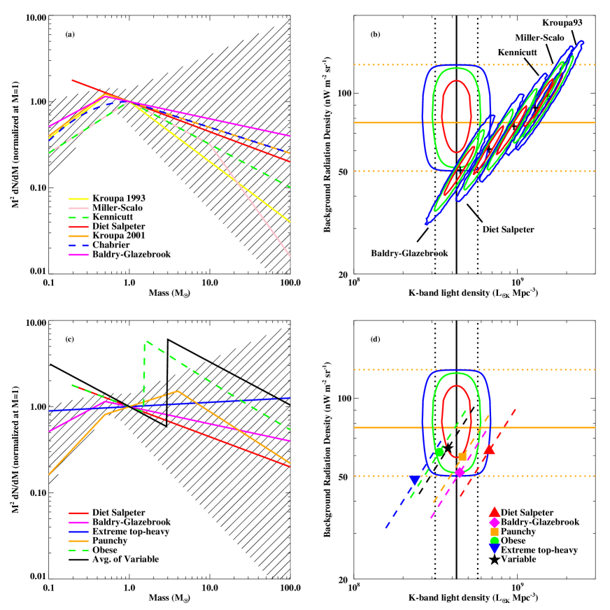
Figure 7: (a) The standard IMFs considered in the paper. The vertical axis is the mass contained in the IMF per unit logarithmic stellar mass. The shaded region is the allowed region taken from Kroupa (2002). (b) The same as Figure 5 but showing the effects of using the different IMFs in the previous panel. We scale each SFH to account for the UV luminosity in a $10^{8}\,\mbox{yr}$ burst for that particular IMF. The contours reflect a systematic error of $\sigma_{A}=0.2$ in the SFH calibration. (c) Shows the new IMFs introduced in the paper. We also plot Baldry-Glazebrook as an example of a moderately top-heavy IMF and Diet Salpeter for comparison. (d) Like panel (b) but for the IMFs shown in panel (c). To avoid the confusion of overlapping contours, we only show the values from the best fit and indicate the approximate contour extent by a dashed line.

In Figure 7a we show several IMFs that have been proposed in the literature (Salpeter, 1955; Miller & Scalo, 1979; Kennicutt, 1983; Kroupa et al., 1993; Kroupa, 2001; Chabrier, 2003; Baldry & Glazebrook, 2003), all normalised to the same value at $1\,M_{\sun}$. We also show the approximate allowed region of the IMF as determined by Kroupa (2002). This allowed region was established from studies using several different techniques covering different mass ranges; hence the normalisations above and below $1\,M_{\sun}$ are poorly constrained relative to one another. The slopes from 1 to $15\,M_{\sun}$ in the plot are 1.7 for Kroupa (1993), 1.6 for Miller-Scalo (1979), 1.5 for Kennicutt (1983), 1.35 for Salpeter (1955), 1.3 for Kroupa (2001, mean Galactic-field form in Equation 2) and Chabrier (2003), and 1.2 for Baldry & Glazebrook (2003) IMFs.

Now let us repeat the exercise leading to Figure 5 but using the different IMFs. We normalise the star formation histories by the amount of UV light produced in a $10^{8}\,\mbox{yr}$ burst. (Using the bolometric luminosity at the same burst length would give a similar scaling.) Figure 7b shows the resulting $K$-band-$J_{\it EBL}$ contours. There is a single overall trend in this plot. The stars that dominate the $K$-band light today ($\rho_{K}$), the EBL, and the UV light are of progressively higher mass, so as the IMF slope above $1\,M_{\sun}$ is made shallower, the contours shift to lower values of $\rho_{K}$ and $J_{\it EBL}$, while at the same time the ratio of $J_{\it EBL}/\rho_{K}$ increases. (Changes to the IMF below $1\,M_{\sun}$ have little effect on the $K$-band or bolometric light.) Because $\rho_{K}$ is most likely better known than the calibration of the SFH, making the IMF shallower above $1\,M_{\sun}$ actually raises the most plausible background value, despite the resulting decline in the mean $J_{\it EBL}$ of the contours.

We consider the Salpeter IMF to be the point at which the agreement is marginally acceptable, and rule out IMF slopes steeper than the Salpeter value of $-1.35$. This excludes a number of IMFs commonly used in the literature. The Baldry & Glazebrook (2003) IMF is the most acceptable; these authors estimate a high-mass slope of $-1.15\pm 0.2$, which independently rules out the steepest IMFs. Alone among the IMFs in Figure 7b, the Baldry-Glazebrook IMF was derived from the global SFH, in this case by comparing the spectrum of the local luminosity density to observationally plausible shapes of the SFH. It is interesting that it agrees best with our independent test, perhaps indicating that the estimates from Galactic data are somehow biased or that the Galactic IMF differs from the Universal average.

However, none of the standard IMFs from the literature give more than marginal agreement with our joint contours in $\rho_{K}$ and $J_{\it EBL}$. This will pose a problem if future observations constrain the background to a high value. We now consider several examples to see what is required to get significantly higher levels of background light.

We first consider the case of universal IMFs. For our purposes this does not necessarily imply a completely invariant IMF from one galaxy to another, but does require that there be no systematic change with redshift. It is useful to distinguish between a top-heavy IMF, rich in high-mass ($M>8\,M_{\sun}$) stars relative to Sun-like stars, and a middle-heavy or “paunchy” IMF, rich in intermediate-mass ($1\,M_{\sun}<M<8\,M_{\sun}$) stars. As discussed above, the particular range that would be most efficient in boosting $J_{\it EBL}$ relative to the UV/FIR or $K$-band light is 1.5–$4\,M_{\sun}$.

In Figure 7c and Table 1 we introduce three additional IMFs. The first is an “extreme top-heavy” IMF (the slope here is $0.95$, so that the mass converges only at the upper end of the mass function). As an example of a “paunchy” IMF, we place a break at $4\,M_{\sun}$, and for a more extreme or “obese” example, we place a discontinuity at $1.5\,M_{\sun}$. For comparison, we also include a diet Salpeter IMF, and we use the Baldry-Glazebrook IMF as an example of a modestly top-heavy IMF.

We plot results in the $\rho_{K}$-$J_{\it EBL}$ plane for these IMFs in Figure 7d. Here, we only represent the results in a schematic way to avoid overlapping contours. The top-heavy examples continue the general trend down and to the left in the plot. The paunchy examples, by contrast, go only to the left since they have enhanced bolometric emission relative to the $K$-band or UV light.

Our paunchy and extreme top-heavy IMFs reside within the hatched allowed regions of Kroupa (2001) and Kroupa (2002). For 0.5–$1.0\,M_{\sun}$, the paunchy IMF is in marginal conflict with Kroupa’s limits on the slope, but this is based on only a few samples with large error bars and potentially large systematics. The Baldry-Glazebrook and extreme top-heavy IMFs are in good agreement with all of these limits. The obese IMF, however, is too “paunchy” to be consistent with Milky Way observations.

The need to join together estimates in different mass ranges from different environments into a single IMF contributes to an uncertainty in the observed shape of the IMF (Massey, 1998; Kroupa, 2002; Chabrier, 2003; Lada & Lada, 2003). As shown in Figure 5 of Kroupa (2002), estimates of the slope in the range 0.8–$3\,M_{\sun}$ show a particularly large scatter, because neither the Galactic field star or young cluster methods is very effective in this region. Kroupa notes that the low and high mass regions of the IMF are observationally almost disjoint, owing to the lack of overlap between the mass ranges of the most accurate methods. Thus if anything, the hatched regions in Figures 7a and 7c are too restrictive in the region around $1\,M_{\sun}$, making a paunchy IMF more plausible. For example, Sirianni et al. (2000) used HST photometry of the large star cluster 30 Dor in the LMC to obtain isochrones in the colour-magnitude diagram. Their resulting IMF has a slope of $1.28\pm 0.03$ for $M>2.1\,M_{\sun}$, and $0.27\pm 0.08$ for $M<2.1\,M_{\sun}$, at least down to $1.3\,M_{\sun}$ where the noise becomes large. This is tentative support for a paunchy IMF, at least in some active star-forming environments, which may be more representative of the main contributors to the cosmic SFH.

Interestingly, Kroupa (2001) finds evidence for a larger number of low-mass stars in the present-day IMF than in the mean Galactic IMF, which is dominated by stars formed within the last $5\,\mbox{Gyr}$. This is tentative evidence that the IMF has been increasingly weighted to stars above $1\,M_{\sun}$ in the past, and it would not be surprising if the trend continued to the global population of stars, which is still older on average than the local Galactic disk.

Let us now consider an IMF that varies systematically with cosmic time. There are both theoretical and observational motivations for considering a top-heavy IMF for high-redshift or high-SFR galaxies. Problems that this has been invoked to solve include gas consumption timescales in starbursts (Rieke, Loken, Rieke, & Tamblyn, 1993), systematic variations of metallicity and $M/L$ ratios in ellipticals (Zepf & Silk, 1996), and large iron abundances in clusters (Zepf & Silk, 1996; Maoz & Gal-Yam, 2004). It has often been suggested that in extreme star formation environments, the formation of low-mass stars should be suppressed either by the global increased temperature of the medium, which basically raises the Jeans mass, or by feedback from high-mass stars (Massey, 1998; Larson, 1998). However, proving this by observing low and high mass stars together in the same environment is very difficult. Simulations suggest that primordial metal-free stars, at least, form with an extremely top-heavy IMF (with a minimum mass $\sim\!100\,M_{\sun}$; Abel, Bryan, & Norman, 2002), while simulations of starburst galaxies also suggest a top-heavy IMF (Padoan, Nordlund, & Jones, 1997). The Milky Way IMF shows two characteristic mass scales, at $\sim\!0.01$ and $\sim\!0.5\,M_{\sun}$ (Kroupa, 2001), whose origin is not well understood. It would not be surprising if these characteristic masses shifted with redshift, metallicity, or SFR.

As a toy model to investigate this idea, we suppose that there are both “normal” and “rapid” modes of star formation and associate the latter with starbursting galaxies, making it much more important at high redshifts (cf. Lagache et al., 2003). We assume both modes have a Kennicutt IMF, but sharply truncate it in the “rapid” mode below $3\,M_{\sun}$. We assume that the normal mode contributes a fixed amount of star formation at all redshifts, which is 90% of the star formation rate today, and that the rapid mode contributes the remainder. In this model the rapid mode quickly becomes the dominant form as the redshift increases. At very high redshifts, where the SFR rate falls below 90% of the rate today, we just assume that all the star formation is in the normal mode. Each component is scaled according to its UV luminosity at $10^{8}\,\mbox{yr}$ to match the specified fraction of the best-fit SFH.

We show the time-averaged IMF produced by this toy model in Figure 7c, and its resulting location in the $\rho_{K}$-$J_{\it EBL}$ plane in Figure 7d. Clearly, this type of model can produce large background levels, especially if the calibration of the SFH is poorly known at high redshift. We note that from an energetic standpoint this is an inefficient solution, since much of the large energy output at early times is redshifted away. It would be more efficient to make the top-heavy mode dominant at low redshift, but this would then lead to conflicts with local observational constraints on the IMF. This particular model can be described as paunchy, since it has a sudden jump at $3\,M_{\sun}$.

We conclude that a paunchy or top-heavy IMF is observationally allowed, and might indeed be required to solve the background problem, depending on how future observations sort themselves out. The consequences of a top-heavy IMF have been frequently considered. A paunchy IMF also has numerous consequences, which are similar in some ways and different in others to a top-heavy IMF. For a given SFH, it increases the number of F, A, and late B main-sequence stars and the number of bright giants. This will increase the optical brightness of galaxies relative to the IR, or raise the specific SFR that is inferred assuming a standard IMF. Currently, the SFH deduced from the fossil record is significantly higher than direct SFH measurements at lookback times of $\sim\!5\,\mbox{Gyr}$, and significantly lower at $\la 1\,\mbox{Gyr}$ and $\ga 8\,\mbox{Gyr}$ (Heavens et al., 2004). This suggests that there are fewer low-mass and high-mass stars than one expects from simply integrating the observed SFH, assuming a standard IMF. Assuming a paunchy IMF would help solve this discrepancy.

With a paunchy IMF, post-starburst “E$+$A” galaxies will appear more frequently. The cosmic luminosity density will also be modified, and it would be worthwhile to repeat the analysis of Baldry & Glazebrook (2003), with a break at intermediate stellar masses, to see whether the high-mass slope we have assumed for the paunchy form could be constrained. The passive evolution of galaxies would appear more rapid with a paunchy IMF, so that the apparent mass function of high-redshift red-sequence galaxies would shift to higher masses than if one assumed a standard IMF. The intermediate-mass stars will leave large numbers of white dwarfs, amounting to $\sim\!20\%$ of the total stellar mass, which could be constrained by microlensing surveys. Finally, the chemical byproducts of intermediate-mass stars are very different from those of high-mass stars, tending to make “$\alpha$-suppressed” abundances. Hence, the analysis of cosmic abundances may be able to place limits on the shape of this type of IMF.

6 CONCLUSIONS

We have investigated the relationship between the total amount of extragalactic background light, the cosmic star formation history, and the stellar population today. We find that there is tension, and arguably outright conflict, between the background light and NIR surveys that probe the local stellar mass density around $1\,M_{\sun}$, if we assume a standard Salpeter IMF slope. We have paid particular attention to uncertainty in the star formation history; we find that it contributes only a small dispersion to the predicted ratio of background light and NIR light, even though the total amount of star formation is highly uncertain.

This ratio, however, is IMF-dependent. Universal IMFs with steeper slopes above $1\,M_{\sun}$, such as Kennicutt (1983), Miller & Scalo (1979), or Kroupa et al. (1993), are ruled out by the current minimum energy requirements. If the higher absolute background measurements should be substantiated in the future, it conversely implies that the average IMF is slightly top-heavy, or more likely (given limits on the observed star formation history), middle-heavy or “paunchy”, i.e. rich in 1.5–$4\,M_{\sun}$ stars compared to the Salpeter IMF. Alternative solutions in which non-stellar sources make large contributions to the background light appear unlikely.

We note that every quantity that one can measure for the stellar population of galaxies is IMF-dependent, and many secondary conclusions drawn from the study of galactic stellar populations, e.g. galaxy merger rates or rates of gas infall, depend in an indirect way on the IMF. The extreme difficulty of deriving the stellar IMF from first principles, the fundamental difficulty of establishing the IMF above $1\,M_{\sun}$ from local observations, and the theoretical suspicion that the IMF varies with environment all suggest that galactic astronomers may have to deduce the form of the IMF from their own data. For that, we will need to develop good tests involving closed systems of gas and stars. Since the Universe is the ultimate closed system, it seems likely that studies of cosmic-averaged quantities will be crucial to establish the form of the IMF. The study of cosmic star formation and background light in this paper is a step in that direction.

We thank Martin Weinberg, Andrew Hopkins, Harry Ferguson, Eric Bell, Mauro Giavalisco, Laura Silva, Ben Panter, and Steve Schneider for useful conversations. This research was supported by NASA grants NAG5-13102, NAGS-13308, and NNG04GK68G, and NSF grant AST-0205969.

References

- Abel, Bryan, & Norman (2002) Abel, T., Bryan, G. L., & Norman, M. L. 2002, Science, 295, 93
- Aharonian (2001) Aharonian, F. A. 2001, International Cosmic Ray Conference, 27, 250 (astro-ph/0112314)
- Aharonian et al. (2002) Aharonian, F. et al. 2002, A&A, 384, L23
- Aharonian et al. (2005) Aharonian, F. et al. 2005, Nature, accepted (astro-ph/0508073)
- Aller & Richstone (2002) Aller, M. C., & Richstone, D. 2002, AJ, 124, 3035
- Baldry & Glazebrook (2003) Baldry, I. K., & Glazebrook, K. 2003, ApJ, 593, 258
- Barger, Cowie, & Richards (2000) Barger, A. J., Cowie, L. L., & Richards, E. A. 2000, AJ, 119, 2092
- Bell & de Jong (2001) Bell, E. F., & de Jong, R. S. 2001, ApJ, 550, 212
- Bell et al. (2003) Bell, E. F., McIntosh, D. H., Katz, N., & Weinberg, M. D. 2003, ApJS, 149, 289
- Bernstein, Freedman, & Madore (2002a) Bernstein, R. A., Freedman, W. L., & Madore, B. F. 2002, ApJ, 571, 56
- Bernstein, Freedman, & Madore (2002b) Bernstein, R. A., Freedman, W. L., & Madore, B. F. 2002, ApJ, 571, 107
- Bouwens et al. (2006) Bouwens, R. J., Illingworth, G. D., Blakeslee, J. P., Franx, M. 2006, ApJ, accepted (astro-ph/0509641)
- Brinchmann & Ellis (2000) Brinchmann, J., & Ellis, R. S. 2000, ApJ, 536, L77
- Bruzual & Charlot (2003) Bruzual, G., & Charlot, S. 2003, MNRAS, 344, 1000
- Bullock et al. (2000) Bullock, J. S., Kravtsov, A. V., & Weinberg, D. H. 2000, ApJ, 539, 517
- Calzetti (1999) Calzetti, D. 1999, Ap&SS, 266, 243 (astro-ph/9902107)
- Cambrésy et al. (2001) Cambrésy, L., Reach, W. T., Beichman, C. A., & Jarrett, T. H. 2001, ApJ, 555, 563
- Chabrier (2003) Chabrier, G. 2003, PASP, 115, 763
- Chapman et al. (2005) Chapman, S. C., Blain, A. W., Smail, I., & Ivison, R. J. 2005, ApJ, 622, 772
- Cole et al. (2000) Cole, S., Lacey, C. G., Baugh, C. M., & Frenk, C. S. 2000, MNRAS, 319, 168
- Cole et al. (2001) Cole, S. et al. 2001, MNRAS, 326, 255
- Connolly et al. (1997) Connolly, A. J., Szalay, A. S., Dickinson, M., Subbarao, M. U., & Brunner, R. J. 1997, ApJ, 486, L11
- Dekel & Birnboim (2006) Dekel, A., & Birnboim, Y. 2006, MNRAS, 368, 2
- Dickinson et al. (2003) Dickinson, M., Papovich, C., Ferguson, H. C., Budavari, T. 2003, ApJ, 587, 25
- Dole et al. (2006) Dole, H., et al. 2006, A&A, accepted (astro-ph/0603208)
- Drory et al. (2004) Drory, N., Bender, R., Feulner, G., Hopp, U., Maraston, C., Snigula, J., & Hill, G. J. 2004, ApJ, 608, 742
- Drory et al. (2005) Drory, N., Salvato, M., Gabasch, A., Bender, R., Hopp, U., Feulner, G., & Pannella, M. 2005, ApJ, 619, L131
- Dwek et al. (2005) Dwek, E., Arendt, R. G., & Krennrich, F. 2005, ApJ, 635, 784
- Durrell et al. (2002) Durrell, P. R., Ciardullo, R., Feldmeier, J. J., Jacoby, G. H., & Sigurdsson, S. 2002, ApJ, 570, 119
- Eke et al. (2005) Eke, V. R., Baugh, C. M., Cole, S., Frenk, C. S., King, H. M., & Peacock, J. A. 2005, MNRAS, 362, 1233
- Fazio et al. (2004) Fazio, G. G., et al. 2004, ApJS, 154, 39
- Fioc & Rocca-Volmerange (1997) Fioc, M. & Rocca-Volmerange, B. 1997, A&A, 326, 950
- Finkbeiner et al. (2000) Finkbeiner, D. P., Davis, M., & Schlegel, D. J. 2000, ApJ, 544, 81
- Fixsen et al. (1998) Fixsen, D. J., Dwek, E., Mather, J. C., Bennett, C. L., & Shafer, R. A. 1998, ApJ, 508, 123
- Fontana et al. (2003) Fontana, A., et al. 2003, ApJ, 594, L9
- Fontana et al. (2004) Fontana, A., et al. 2004, A&A, 424, 23
- Fukugita, Hogan, & Peebles (1998) Fukugita, M., Hogan, C. J., & Peebles, P. J. E. 1998, ApJ, 503, 518
- Fukugita & Peebles (2004) Fukugita, M., & Peebles, P. J. E. 2004, ApJ, 616, 643
- Gabasch et al. (2004) Gabasch, A., et al. 2004, ApJ, 616, L83
- Gallego et al. (1995) Gallego, J., Zamorano, J., Aragon-Salamanca, A., & Rego, M. 1995, ApJ, 455, L1
- Giavalisco et al. (2004) Giavalisco, M., et al. 2004, ApJ, 600, L103
- Gispert, Lagache, & Puget (2000) Gispert, R., Lagache, G., & Puget, J. L. 2000, A&A, 360, 1
- Gould, Bahcall, & Flynn (1996) Gould, A., Bahcall, J. N., & Flynn, C. 1996, ApJ, 465, 759
- Gnedin (2000) Gnedin, N. Y. 2000, ApJ, 542, 535
- Gorjian et al. (2000) Gorjian, V., Wright, E. L., & Chary, R. R. 2000, ApJ, 536, 550
- Graham & Driver (2005) Graham, A. W., & Driver, S. P. 2005, Publications of the Astronomical Society of Australia, 22, 118
- Guhathakurta et al. (2005) Guhathakurta, P., Rich, R. M., Reitzel, D. B., Cooper, M. C., Gilbert, K., Majewski, S. R., Ostheimer, J. C., Geha, M. C., Johnston, K. V., & Patterson, R. J. 2005, AJ, submitted (astro-ph/0406145)
- Gwyn & Hartwick (2005) Gwyn, S. D. J., & Hartwick, F. D. A. 2005, AJ, 130, 1337
- Hauser et al. (1998) Hauser, M. G., et al. 1998, ApJ, 508, 25
- Hauser & Dwek (2001) Hauser, M. G., & Dwek, E. 2001, ARA&A, 39, 249
- Heavens et al. (2004) Heavens, A., Panter, B., Jimenez, R., & Dunlop, J. 2004, Nat, 428, 625
- Hopkins et al. (2000) Hopkins, A. M., Connolly, A. J., & Szalay, A. S. 2000, AJ, 120, 2843
- Hopkins & Beacom (2006) Hopkins, A. M., & Beacom, J. F. 2006, submitted to ApJ, astro-ph/0601463
- Hopkins (2004) Hopkins, A. M. 2004, ApJ, 615, 209
- Hopkins et al. (2006) Hopkins, P. Laas, & co. 2006, ApJS, accepted (astro-ph/0506398)
- Jones et al. (2006) Jones, D. H., Peterson, B. A., Colless, M., Saunders, W. 2006, accepted to MNRAS (astro-ph/0603609)
- Kashlinsky et al. (1996a) Kashlinsky, A., Mather, J. C., Odenwald, S., & Hauser, M. G. 1996, ApJ, 470, 681
- Kashlinsky et al. (1996b) Kashlinsky, A., Mather, J. C., & Odenwald, S. 1996, ApJ, 473, L9
- Kashlinsky & Odenwald (2000) Kashlinsky, A., & Odenwald, S. 2000, ApJ, 528, 74
- Katz et al. (1992) Katz, N., Hernquist, L., & Weinberg, D. H. 1992, ApJ, 399, L109
- Kauffmann et al. (1999) Kauffmann, G., Colberg, J. M., Diaferio, A., & White, S. D. M. 1999, MNRAS, 303, 188
- Kennicutt (1983) Kennicutt, R. C. 1983, ApJ, 272, 54
- Kereš et al. (2005) Kereš, D., Katz, N., Weinberg, D. H., & Davé, R. 2005, MNRAS, 363, 2
- Kroupa et al. (1993) Kroupa, P., Tout, C. A., & Gilmore, G. 1993, MNRAS, 262, 545
- Kroupa (2001) Kroupa, P. 2001, MNRAS, 322, 231
- Kroupa (2002) Kroupa, P. 2002, Science, 295, 82
- Lada & Lada (2003) Lada, C. J., & Lada, E. A. 2003, ARA&A, 41, 57
- Lagache et al. (2000) Lagache, G., Haffner, L. M., Reynolds, R. J., & Tufte, S. L. 2000, A&A, 354, 247
- Lagache et al. (2003) Lagache, G., Dole, H., & Puget, J.-L. 2003, MNRAS, 338, 555
- Larson (1998) Larson, R. B. 1998, MNRAS, 301, 569
- Madau et al. (1996) Madau, P., Ferguson, H. C., Dickinson, M. E., Giavalisco, M., Steidel, C. C., & Fruchter, A. 1996, MNRAS, 283, 1388
- Madau & Pozzetti (2000) Madau, P. & Pozzetti, L. 2000, MNRAS, 312, L9
- Madau et al. (2001) Madau, P., Haardt, F., & Pozzetti, L. 2001, IAU Symposium, 204, 359
- Madau & Silk (2005) Madau, P., & Silk, J. 2005, MNRAS, 359, L37
- Marconi et al. (2004) Marconi, A., Risaliti, G., Gilli, R., Hunt, L. K., Maiolino, R., & Salvati, M. 2004, MNRAS, 351, 169
- Martin et al. (2005) Martin, D. C., et al. 2005, ApJ, 619, L59
- Massey (1998) Massey, P. 1998, ASP Conf. Ser. 142: The Stellar Initial Mass Function (38th Herstmonceux Conference), 142, 17
- Matsumoto et al. (2005) Matsumoto, T., et al. 2005, ApJ, 626, 31
- Maoz & Gal-Yam (2004) Maoz, D., & Gal-Yam, A. 2004, MNRAS, 347, 951
- Miller & Scalo (1979) Miller, G. E., & Scalo, J. M. 1979, ApJS, 41, 513
- Mouhcine et al. (2005) Mouhcine, M., Ferguson, H. C., Rich, R. M., Brown, T. M., & Smith, T. E. 2005, ApJ, 633, 821
- Nagamine et al. (2000) Nagamine, K., Cen, R., & Ostriker, J. P. 2000, ApJ, 541, 25
- Nagamine et al. (2006) Nagamine, K., Ostriker, J. P., Cen, R., & Fukugita, M. 2000, ApJ, submitted (astro-ph/0603257)
- Padoan, Nordlund, & Jones (1997) Padoan, P., Nordlund, A., & Jones, B. J. T. 1997, MNRAS, 288, 145
- Okamura et al. (2002) Okamura, S. et al. 2002, PASJ, 54, 883
- Panter et al. (2003) Panter, B., Heavens, A. F., & Jimenez, R. 2003, MNRAS, 343, 1145
- Panter et al. (2004) Panter, B., Heavens, A. F., & Jimenez, R. 2004, MNRAS, 355, 764
- Papovich et al. (2004) Papovich, C., et al. 2004, ApJS, 154, 70
- Pérez-González et al. (2003) Pérez-González, P. G., Zamorano, J., Gallego, J., Aragón-Salamanca, A., & Gil de Paz, A. 2003, ApJ, 591, 827
- Pérez-González et al. (2005) Pérez-González, P. G., et al. 2005, ApJ, 630, 82
- Pozzetti & Madau (2001) Pozzetti, L., & Madau, P. 2001, IAU Symposium (astro-ph/0011359)
- Primack et al. (2005) Primack, J. R., Bullock, J. S., & Somerville, R. S. 2005, AIP Conf. Proc. 745: High Energy Gamma-Ray Astronomy, 745, 23
- Salpeter (1955) Salpeter, E. E. 1955, ApJ, 121, 161
- Salvaterra & Ferrara (2006) Salvaterra, R., & Ferrara, A. 2006, MNRAS, 216
- Schiminovich et al. (2005) Schiminovich, D., et al. 2005, ApJ, 619, L47
- Rieke, Loken, Rieke, & Tamblyn (1993) Rieke, G. H., Loken, K., Rieke, M. J., & Tamblyn, P. 1993, ApJ, 412, 99
- Santos et al. (2002) Santos, M. R., Bromm, V., & Kamionkowski, M. 2002, MNRAS, 336, 1082
- Sawicki & Thompson (2005) Sawicki, M., & Thompson, D. 2005, ApJ, 635, 100
- Silva et al. (2004) Silva, L., Maiolino, R., & Granato, G. L. 2004, MNRAS, 355, 973
- Sirianni et al. (2000) Sirianni, M., Nota, A., Leitherer, C., De Marchi, G., & Clampin, M. 2000, ApJ, 533, 203
- Soltan (1982) Soltan, A. 1982, MNRAS, 200, 115
- Somerville, Primack, & Faber (2001) Somerville, R. S., Primack, J. R., & Faber, S. M. 2001, MNRAS, 320, 504
- Spergel et al. (2006) Spergel, D. N., et al. 2006, submitted to ApJ (astro-ph/0603449)
- Springel & Hernquist (2003) Springel, V. & Hernquist, L. 2003, MNRAS, 339, 312
- Springel et al. (2005) Springel, V., Di Matteo, T., & Hernquist, L. 2005, ApJ, 620, L79
- Steidel et al. (1999) Steidel, C. C., Adelberger, K. L., Giavalisco, M., Dickinson, M., & Pettini, M. 1999, ApJ, 519, 1
- Strauss et al. (2002) Strauss, M.A., et al. 2002, AJ, 124, 1810
- Sullivan et al. (2000) Sullivan, M., Treyer, M. A., Ellis, R. S., Bridges, T. J., Milliard, B., & Donas, J. ; 2000, MNRAS, 312, 442
- Tapken al. (2006) Tapken, C., et al. 2006, A&A, accepted (astro-ph/0604262)
- Treister et al. (2006) Treister, E., et al. 2006, ApJ, 640, 603
- Tresse & Maddox (1998) Tresse, L. & Maddox, S. J. 1998, ApJ, 495, 691
- Tresse et al. (2002) Tresse, L., Maddox, S. J., Le Fèvre, O., & Cuby, J.-G. 2002, MNRAS, 337, 369
- Tumlinson et al. (2004) Tumlinson, J., Venkatesan, A., & Shull, J. M. 2004, ApJ, 612, 602
- Webb et al. (2006) Webb, T. M. A., et al. 2006, ApJ, 636, L17
- Wolf et al. (2003) Wolf, C., Meisenheimer, K., Rix, H.-W., Borch, A., Dye, S., & Kleinheinrich, M. 2003, A&A, 401, 73
- Wright (2001) Wright, E. L. 2001, ApJ, 553, 538
- Wright (2004) Wright, E. L. 2004, New Astronomy Review, 48, 465
- Wolfe et al. (2003) Wolfe, A. M., Gawiser, E., & Prochaska, J. X. 2003, ApJ, 593, 235
- Worthey (1994) Worthey, G. 1994, ApJS, 95, 107
- Wright & Reese (2000) Wright, E. L., & Reese, E. D. 2000, ApJ, 545, 43
- Yan et al. (1999) Yan, L., McCarthy, P. J., Freudling, W., Teplitz, H. I., Malumuth, E. M., Weymann, R. J., & Malkan, M. A. 1999, ApJ, 519, L47
- Yun, Reddy, & Condon (2001) Yun, M. S., Reddy, N. A., & Condon, J. J. 2001, ApJ, 554, 803
- Zepf & Silk (1996) Zepf, S. E. & Silk, J. 1996, ApJ, 466, 114