The O VII X-ray forest toward Markarian 421: Consistency between XMM-Newton and Chandra

Abstract

Recently the first detections of highly ionised gas associated with two Warm-Hot Intergalactic Medium (WHIM) filaments have been reported. The evidence is based on X-ray absorption lines due to O VII and other ions observed by Chandra towards the bright blazar Mrk 421. We investigate the robustness of this detection by a re-analysis of the original Chandra LETGS spectra, the analysis of a large set of XMM-Newton RGS spectra of Mrk 421, and additional Chandra observations. We address the reliability of individual spectral features belonging to the absorption components, and assess the significance of the detection of these components. We also use Monte Carlo simulations of spectra. We confirm the apparent strength of several features in the Chandra spectra, but demonstrate that they are statistically not significant. This decreased significance is due to the number of redshift trials that are made and that are not taken into account in the original discovery paper. Therefore these features must be attributed to statistical fluctuations. This is confirmed by the RGS spectra, which have a higher signal to noise ratio than the Chandra spectra, but do not show features at the same wavelengths. Finally, we show that the possible association with a Ly$\alpha$ absorption system also lacks sufficient statistical evidence. We conclude that there is insufficient observational proof for the existence of the two proposed WHIM filaments towards Mrk 421, the brightest X-ray blazar on the sky. Therefore, the highly ionised component of the WHIM still remains to be discovered.

1 Introduction

Cosmological simulations show that the matter in the Universe is not uniformly distributed but forms a web-like structure. Clusters of galaxies and superclusters are found at the knots of this cosmic web. They are the location of the highest mass concentration. The knots are connected through diffuse filaments, containing a mixture of dark matter, galaxies and gas. According to these simulations, the major part of this gas should be in a low density, intermediate temperature ($10^{5}$ – $10^{7}$ K) phase, the so-called Warm-Hot Intergalactic Medium (WHIM, Cen & Ostriker cen1999 (1999)). About half of all baryons in the present day Universe should reside in this WHIM according to the theoretical predictions, yet little of it has been seen so far. As the physics of the WHIM is complicated and many processes are relevant to its properties, observations of the WHIM are urgently needed.

The density of the WHIM is low (typically 1 – 1000 times the average baryon density of the Universe (for example Davé et al. dave2001 (2001)) or 0.3 – 300 m^-3) and the temperature is such that most emission will occur in the EUV band. As the EUV band is strongly absorbed by the neutral hydrogen of our Galaxy and its thermal emission is proportional to density squared, only the hottest and most dense part of the WHIM can be observed in emission with X-ray observatories such as XMM-Newton. Indications of O VII line emission from the WHIM near clusters have been reported now (Kaastra et al. kaastra2003 (2003), Finoguenov et al. finoguenov2003 (2003)).

It is also possible to observe the WHIM in absorption, provided that a strong background continuum source is present and provided a high-resolution spectrograph is used. The first unambiguous detections of the WHIM in absorption have been made in the UV band using bright quasar absorption lines from O VI as observed with the Far Ultraviolet Spectroscopic Explorer (FUSE) satellite (Tripp et al. tripp2000 (2000); Oegerle et al. oegerle2000 (2000); Savage et al. savage2002 (2002); Jenkins et al. jenkins2003 (2003)).

Observation in the UV band is relatively easy because of the high spectral resolution of FUSE and the relatively long wavelength $\lambda$ of the UV lines. Since the optical depth at line centre scales proportional to the wavelength and the best spectral resolution of the current X-ray observatories is an order of magnitude poorer than FUSE, X-ray absorption lines are much harder to detect.

The first solid detection of X-ray absorption lines at $z=0$ towards a quasar has been made by Nicastro et al. nicastro2002 (2002). A spectrum of the bright quasar PKS 2155$-$304 (catalog ) taken with the Low Energy Transmission Grating Spectrometer (LETGS) of Chandra showed zero redshift absorption lines due to O VII, O VIII and Ne IX. These lines have been confirmed by XMM-Newton Reflection Grating Spectrometer (RGS) observations (Paerels et al. paerels2003 (2003); Cagnoni et al. cagnoni2003 (2003)), and similar X-ray absorption lines have been seen towards several other sources, for example 3C 273 (catalog ), Fang et al. fang2003 (2003); NGC 5548 (catalog ), Steenbrugge et al. steenbrugge2003 (2003); NGC 4593 (catalog ), McKernan et al. mckernan2003 (2003); and Mrk 279 (catalog ), Kaastra et al. kaastra2004 (2004). However, whether these lines are due to the local WHIM (for instance around our Local Group) or that these lines have a Galactic origin is still debated.

Therefore, the first unambiguous proof of X-ray absorption lines from the WHIM has to come from $z>0$ absorption lines. A first report of a $z=0.055$ X-ray absorption system towards PKS 2155$-$304 (catalog ) has been given by Fang et al. fang2002 (2002) using a Chandra LETG/ACIS observation. However, this feature must be either a transient feature and therefore not associated to the WHIM, or an instrumental artifact. This is because these results have not been confirmed in both the more sensitive RGS observations towards this source (Paerels et al. paerels2003 (2003); Cagnoni et al. cagnoni2003 (2003)), nor in a long exposure using the LETG/HRC-S configuration. The X-ray detection of 6 intervening UV absorption systems towards H 1821$+$643 (catalog ) in a 500 ks Chandra observation by Mathur et al. mathur2003 (2003) should best be regarded as an upper limit due to the rather low significance of these detections.

An apparently more robust detection of $z>0$ X-ray absorption due to the WHIM has been presented by Nicastro et al. (2005a , 2005b , NME herafter). These authors observed the brightest blazar on the sky, Mrk 421 (catalog ), when the source was in outburst, typically an order of magnitude brighter than the average state of this source. They obtained two high-quality Chandra LETGS spectra of Mrk 421. They report the detection of two intervening X-ray absorption systems towards this source in the combined spectra. The first one at $z=0.011$ with a significance of 5.8$\sigma$ was associated with a known H I Ly$\alpha$ system, and the second one at $z=0.027$ with a significance of 8.9$\sigma$ was associated with an intervening filament $\sim 13$ Mpc from the blazar.

The cosmological implications of the detection of the first X-ray forest are perhaps the most important clue to resolving the problem of the ”missing baryons” (see Nicastro et al. 2005a ), and therefore the robustness of this detection is extremely important. Mrk 421 has been observed many times by XMM-Newton as part of its routine calibration plan. The total integration time of 950 ks accumulated over all individual observations with a broad range of flux levels yields a spectrum with a quality superior to the Chandra spectra taken during outburst. With such a high signal to noise ratio of the spectra all kinds of systematic effects become important and we have developed a novel way to analyse the RGS spectra taking account of these effects. This new analysis is presented in the accompanying paper (Rasmussen et al. rasmussen2006 (2006)). Here we present a carefull re-analysis of all archival Chandra spectra of this source and compare the results from both instruments.

2 Observations and data analysis

2.1 Analysis of the LETGS spectra

We processed all 7 Chandra LETGS observations of Mrk 421 with a total exposure time of 450 ks (see Table 1). Two deep ($\sim 100$ ks) Chandra LETG/ACIS and LETG/HRC-S observations of Mrk 421 were triggered after outbursts catching the source at its historical maximum. The $\sim 20$ ks LETG/HRC-S observation was obtained in Chandra Director Discretionary Time after 2 weeks of intense activity. The remaining four LETG/ACIS observations were performed for calibration purposes. Our processed spectra contain in total $\sim 10^{7}$ counts. There are also two short observations with the High Energy Transmission Grating Spectrometer (HETGS) of Chandra, but at the relevant wavelengths ($\lambda>20$ Å) the signal to noise ratio of these spectra is too low for our present investigation.

Table 1: Chandra LETGS observations of Mrk 421 (catalog ). The column ”Set” gives the number of the spectral data set into which each observation was combined. The column ”Flux” gives the flux at 20 Å in phot m^-2 s^-1 Å^-1.

Set	Date	Obs.	Detector	Exposure	Flux
		ID		(ks)
1	2000 May 29	1715	HRC-S	19.84	93
2	2002 Oct 26	4148	ACIS-S	96.84	333
1	2003 Jul 01	4149	HRC-S	99.98	242
3	2004 May 06	5318	ACIS-S	30.16	256
3	2004 Jul 12	5331	ACIS-S	69.50	39
3	2004 Jul 13	5171	ACIS-S	67.15	163
3	2004 Jul 14	5332	ACIS-S	67.06	140

The LETG/ACIS spectra were processed with CIAO 3.2.2 (CALDB 2.27) using the standard Chandra X-ray Center pipeline. The spectra and ARFs were combined using the CIAO tool $add\_grating\_spectra$. The LETG/HRC-S spectra were processed as described in detail in Kaastra et al.kaastra2002 (2002).

We combined these seven spectra into three datasets as indicated in Table 1:

1. the $\sim 100$ ks LETG/ACIS observation performed in 2000 when the source had an exceptionally high luminosity (the spectrum contains $\sim 4.3$ million photons)

2. the combined two datasets obtained with LETG/HRC-S in 2000 and 2003 (the spectrum contains $\sim 2.7$ million photons)

3. the combined dataset of 4 calibration observations with LETG/ACIS taken in 2004, when the source was on average at a lower luminosity (the spectrum contains $\sim 3.2$ million counts).

We first analysed spectra 1 & 2, which are the data sets analysed by NME. However, contrary to NME we did not combine these data obtained in different instrument configurations (LETG/ACIS and LETG/HRC-S) and rather decided to fit the spectra simultaneously. For the spectral fitting we used the SPEX package (Kaastra et al. kaastra1996 (1996)). The two spectra obtained with different instrument configurations were fitted with different continuum models but with a common redshift and common absorption components. Since we are interested in weak absorption features and not in the continuum emission of the source, we fitted the underlying continuum with a spline model, using 12 grid points between 9.5–35 Å, with which we also removed any remaining broad instrumental features (for more details on the spline model see the SPEX manual). This spectral range for fitting was chosen because it includes all possible relevant spectral line features from neon, oxygen, nitrogen and carbon.

We modelled the Galactic absorption using the hot model of the SPEX package, which calculates the transmission of a plasma in collisional ionisation equilibrium with cosmic abundances. The transmission of a neutral plasma was mimicked by putting its temperature to 0.5 eV. We fix the Galactic absorption to $1.61\times 10^{24}$ m^-2 (Lockman & Savage lockman1995 (1995)). We fit the absorption lines of the $z=0$ local warm absorber, which is associated with the ISM of our Galaxy or the Local Group WHIM filament, also with the hot model of the SPEX package, but now with the temperature as a free parameter. Our best fit temperature of the local warm absorber is 0.07 keV with a hydrogen column density of $7.4\times 10^{22}$ m^-2.

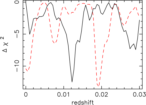
Figure 1: Improvement $\Delta\chi^{2}$ of the fit with weak absorption lines in the model with respect to a fit without these absorption lines, as a function of redshift. Ions included are C VI, N VI, N VII, O VI, O VII, Ne IX, and Ne X. The solid and dashed lines represent the $\Delta\chi^{2}$ distribution as a function of redshift when fitting the observed spectrum and the simulated spectrum respectively.

After obtaining a good fit of the continuum and the local warm absorber we searched for the presence of weak absorption lines in the spectrum. We searched for redshifted absorption lines from C VI, N VI, N VII, O VI, O VII, O VIII, Ne IX, Ne X in all possible WHIM filaments between our Galaxy and Mrk 421. We performed a systematic search for these absorption features. Absorption lines of the above mentioned ions were placed into one of 60 bins corresponding to different redshifts between $z=0$ and $z=0.03$. In each bin the individual column densities of the ions were fitted and the $\Delta\chi^{2}$ of the fit relative to the fit without the weak absorption lines in the model was evaluated. To fit the column densities of the ions we used the slab model of the SPEX package. That model calculates the transmission of a thin slab of matter with arbitrary ionic composition. Free parameters are the velocity broadening $\sigma_{\mathrm{v}}$ which we kept fixed to 100 km s^-1, and the ionic column densities. Note that in our case the column densities are low so we expect to be in the linear part of the curve of growth, such that $\sigma_{\mathrm{v}}$ is irrelevant for the determination of the equivalent width of the absorption lines. In order to really detect weak absorption lines we performed this search with a spacing of 10 mÅ, one fifth of the resolution of the LETGS (50 mÅ). Afterward we simulated a Chandra spectrum with the same exposure time, same continuum model but without the weak absorption features and again performed the same search on the simulated spectrum. The results of the search on the real and on the simulated spectrum are shown in Fig. 1.

We did not include redshifted O VIII lines, since a part of the spectrum where they may be present is influenced by small instrumental uncertainties. In particular a nearby node boundary in LETG/ACIS with small-scale effective area uncertainty would otherwise systematically bias the fit (see Sect. 3.1.1 for more details).

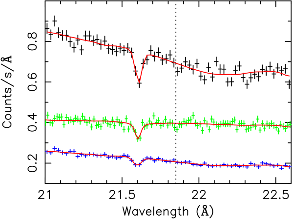
Figure 2: The $21.0-22.6$ Å part of the spectrum of Mrk 421 with its best-fitting continuum model plus an absorption model for the $z=0$ absorber (solid line). The spectrum at the top is the LETG/ACIS observation obtained when the source was in an exceptionally bright state; the spectrum in the middle is the LETG/HRC-S observation obtained in a bright state combined with a short LETG/HRC-S observation obtained at a lower luminosity state; these observations were combined and analysed by NME. The spectrum at the bottom was obtained during 4 calibration observations. The two LETG/ACIS spectra were multiplied by a factor of 1.5 for clarity of display. The dotted line shows the position of the redshifted O VII line observed by NME.

The most significant individual spectral feature which NME interpret as an absorption line from a WHIM filament is the feature associated with an O VII absorption line at z=0.011. To investigate that line further, we considered all three datasets 1–3. We show the $21.0-22.6$ Å spectral interval extracted from these datasets in Fig. 2. The best-fitting continuum model plus an absorption model for the local warm absorber is shown with a solid line and the position of the redshifted O VII line observed by NME is indicated by the vertical dotted line. The spectral feature at 21.85 Å is seen in the spectrum obtained by LETG/HRC-S and a somewhat weaker and shifted feature is seen in the LETG/ACIS spectrum obtained at the high source luminosity. We note that NME combined these two datasets. In the third dataset we do not see any feature at the indicated wavelength, despite the fact that the spectrum contains more photons than the LETG/HRC-S observation.

Finally, we determined the nominal redshift of the $z=0.011$ component from the data sets 1 and 2, using only the strongest absorption lines (O VII 1s–2p). For the $z=0$ O VII line, we measure a line centroid of $21.605\pm 0.006$ and $21.604\pm 0.005$ mÅ for spectrum 1 and 2, respectively; for the $z=0.011$ components these values are $21.864\pm 0.014$ and $21.854\pm 0.011$ mÅ. Therefore, the redshifts of the longer wavelength line with respect to the $z=0$ line is $0.0121\pm 0.0007$ and $0.0117\pm 0.0005$, respectively. The weighted average is $z=0.0118\pm 0.0004$, somewhat higher than the value obtained by NME.

2.2 Analysis of the RGS spectra

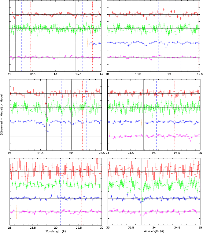
Figure 3: Comparison of the LETGS and RGS spectra of Mrk 421 in the Ne X/Ne IX, O VIII, O VII/O VI, N VII, N VI and C VI bands. Each panel shows from top to bottom the LETG/ACIS spectrum (1), the LETG/HRC-S spectrum, RGS1 and RGS2. The quantities plotted are the fit residuals (observed$-$model)/model with respect to a local continuum model. One tickmark on the y-axis corresponds to 10 %, and the data sets have been shifted arbitrarily along the y-axis in order to avoid overlapping data points. The solid vertical lines correspond to expected features at $z=0$, dashed lines to $z=0.011$, and dash-dotted lines to $z=0.027$. CCD gaps for RGS are shown with dotted lines in the appropriate spectrum. As explained by Rasmussen et al. rasmussen2006 (2006), after careful screening occasionally an isolated instrumental dip may be present in a single RGS, such as at 25.8 Å in RGS2.

The analysis of the RGS spectra is described in detail by Rasmussen et al. rasmussen2006 (2006). We have taken their combined fluxed spectra and corrected these for Galactic absorption using the same hot model of SPEX described above that was used for the LETGS spectra. We adjusted the oxygen column density to $8.5\times 10^{-4}$ of the hydrogen column density in order to get the best match around the oxygen edge. The absorption corrected spectra then were fitted using a spline model with nodes separated by 0.5 Å. Obvious absorption lines were ignored in this continuum fit. This procedure is needed because the statistical quality of our combined data is so good: typically, the flux in the oxygen region is determined with a statistical error of only 0.4 % per 0.5 Å bin. There are remaining, large-scale uncertainties in the RGS effective area of the order of a percent on Å scales that would otherwise bias the spectrum, and moreover to prove that the underlying continuum of all these combined Mrk 421 observations would be a straight power law would be a major challenge. Fig. 3 shows the residuals of this fit in the same 6 wavelength intervals used by NME.

In addition, we show in Fig. 3 the fit residuals of the LETGS spectra 1 and 2, after fitting with the same spline model with with nodes separated by 0.5 Å as was used for the RGS data.

2.3 Determing equivalent widths

Table 2: The formal best-fit equivalent widths ($W_{\lambda}$) in mÅ for absorption lines fixed at wavelengths of 21.60, 21.85, 22.20 and 22.02 Å, corresponding to the expected position of the 1s–2p lines of O VII at $z=0$, $z=0.011$, $z=0.027$, and the 1s–2p doublet of O VI at $z=0$. Negative values indicate emission lines. See the text for the details about the LETGS datasets. We further list $W_{\lambda}$ as derived from the RGS spectra (Sect. 2.2), and the weighted average for all three LETGS data sets and the RGS data (row labelled w.a.). For comparison, we also list the equivalent widths as determined by Williams et al. williams2005 (2005) and NME from the combined LETGS sets 1 and 2 (labelled NME/W). All errors are r.m.s. errors ($\Delta\chi^{2}=2$). The last column gives an estimate of the systematic uncertainty (also in mÅ) on the equivalent widths (not included in the statistical errors).

Dataset	21.60	21.85	22.20	22.02	syst
LETGS 1	$11.6\pm 1.3$	$1.5\pm 1.5$	$3.1\pm 1.5$	$1.9\pm 1.5$	0.6
LETGS 2	$11.7\pm 1.3$	$3.5\pm 1.4$	$-1.5\pm 1.5$	$1.1\pm 1.5$	0.9
LETGS 3	$10.3\pm 1.6$	$-0.6\pm 1.8$	$-0.4\pm 1.9$	$0.1\pm 1.8$	0.6
RGS	$14.8\pm 0.7$	$0.4\pm 0.8$	$-0.6\pm 0.7$	$2.8\pm 0.7$	0.8
w.a.	$13.4\pm 0.5$	$1.0\pm 0.6$	$-0.2\pm 0.6$	$2.1\pm 0.6$
NME/W	$9.4\pm 1.1$	$3.0\pm 0.9$	$2.2\pm 0.8$	$2.4\pm 0.9$

Equivalent widths of selected line features in the 21.0–22.5 Å band were determined from the fit residuals shown in Fig. 3. We consider the $z=0$ line of O VII, as well as the $z=0$ and $z=0.027$ O VII lines and a 22.02 Å feature discussed later. The equivalent widths ($W_{\lambda}$) are given in Table 2.

For RGS1 we used the exact line spread function. Following our earlier work (Kaastra et al. kaastra2002 (2002)), we approximate the lsf of the LETGS by the following analytical formula:

$$\phi\sim 1/[1+(\Delta\lambda/a)^{2}]^{\alpha},$$ (1)

where $\alpha=2$ and $\Delta\lambda$ is the offset from the line centroid. The scale parameter $a$ (expressed here in Å) is weakly wavelength dependent as:

$$a=\sqrt{(0.0313)^{2}+(0.000306\lambda)^{2}}.$$ (2)

The errors on the equivalent widths that we list are simply the statistical errors on the best-fit line normalisation. Table 2 also shows the systematic uncertainties expected for each line due to the uncertainty in the continuum level; these systematic uncertainties were determined by shifting the continuum up and down by the 1$\sigma$ statistical uncertainty in the average continuum flux for each local 0.5 Å  bin and re-determing the equivalent width.

Uncertainties in the shape of the lsf also may affect the derived values of $W_{\lambda}$. We estimated this by modifying the lsf and determining how the equivalent width of the 21.60 Å line changes. For the LETGS, a change of $\alpha$ from 2 (our preferred value) to 2.5 (the value used by the official CIAO software) but keeping the same FWHM by adjusting $a$ leads to a decrease of 0.4 mÅ (3.5 %)in $W_{\lambda}$; a decrease of $a$ by 10 % leads to a decrease of 0.5 mÅ (4.5 %)in $W_{\lambda}$. If for the RGS instead of the true lsf a Gaussian approximation would be used, the equivalent widths would be 20–30 % too small. As shown by Rasmussen et al. rasmussen2006 (2006) the uncertainty in the lsf gives slightly different results ($\sim 10$ %) as two different parameterisations of the lsf are used. For example, decreasing the FWHM of the lsf of the RGS by 10 % leads to a $W_{\lambda}$ decrease of 2.3 mÅ (15 %). Although the precise systematic uncertainty on $W_{\lambda}$ due to the lsf shape is hard to establish accurately, it is most likely in the 5–15 % range for both LETGS and RGS. Taking this into account in addition to the statistical uncertainty on $W_{\lambda}$ and the systematic uncertainty related to the continuum level (Table 2), we conclude that there is not a large discrepancy between the equivalent widths of the $z=0$ O VII line measured by both instruments.

3 Discussion

3.1 Significance of the absorption components detected by Chandra

The evidence for the two absorption components at $z=0.011$ (5.8$\sigma$) and $z=0.027$ (8.9$\sigma$) as presented by NME looks at a first glance convincing. However, there are good reasons to put question marks to these significances. We follow here two routes: first we discuss the significance by looking into detail to the individual features identified by NME, and next we analyse the significance of the absorption components in a coherent way.

3.1.1 Individual line features

NME found 28 or 24 absorption features with a significance of more than 3$\sigma$ in their analysis of the combined LETG/HRC-S and LETG/ACIS spectrum. The precise number is somewhat unclear from their paper but is not important here. Of these 24 lines, 14 have an origin at $z=0$ and there is no doubt about the significance of that component, so we focus on the 10 features with a tentative identification with $z>0$ absorption lines. In total 3 of these belong to the $z=0.011$ system, and 6 to the $z=0.027$ system. One feature at 24.97 Å was unidentified by NME. We will discuss these features here individually as we point out that not all of these detections can be regarded as unambiguous.

The absorption component at $z=0.011$ had three features:

1. O VIII 1s–2p at 19.18 Å: Fig. 3 shows that there is only evidence for an absorption feature from the LETG/ACIS spectrum, not from the LETG/HRC-S or RGS spectra. The feature coincides exactly with a $\sim$ 0.05 Å wide dip of 3 % depth in the effective area of the LETG/ACIS, associated with an ACIS node boundary (as was also pointed out by NME); therefore this feature is most likely of instrumental origin.

2. O VII 1s–2p at 21.85 Å: there is no clear feature in the RGS spectrum, but there is a feature in both LETGS spectra. However, the centroid in the LETG/ACIS spectrum seems to occur at slightly longer wavelength, by $\sim$ 0.01 Å. There are no known instrumental features in the LETGS at this wavelength, so this may be real provided it has sufficient significance. But see Sect. 3.1.2.

3. N VII 1s–2p at 25.04 Å: no feature present in the RGS deeper than 1 %; the LETG/HRC-S spectrum (Fig. 3) shows a $\sim 5$ % negative deviation at a slightly smaller wavelength, and the (here noisy) LETG/ACIS spectrum may be consistent with this. The smaller wavelength is consistent with the findings of NME, who give here a redshift of 0.010 instead of 0.011.

In summary, the X-ray evidence for the 0.011 component rests solely upon the detection of two lines with different redshift and only seen in the LETGS. As we will argue later, even the statistical significance of the combined features is insufficient to designate it as a robust detection.

The component at $z=0.027$ had six features:

1. Ne IX 1s–2p at 13.80 Å: this feature coincides with a narrow dip in the effective area of the LETG/ACIS associated with a node boundary, similar to the $z=0.011$ O VIII 1s–2p line. It is therefore no surprise that it is only seen in the LETG/ACIS spectrum, with perhaps a little but not very significant strengthening from the LETG/HRC-S spectrum. It is not visible in the RGS spectrum. More importantly, its best-fit redshift as reported by NME of 0.026 is off from the redshift of this component at $z=0.027$. We conclude that this feature has an instrumental origin.

2. O VII 1s–3p at 19.11 Å: there is only a weak signal visible in the LETG/HRC-S spectrum (Fig. 3); this looks a little less pronounced than in the plot given by NME but this may be due to different binning; more importantly, given the weakness of the 1s–2p transition in the same ion (see below) and the expected 5 times smaller equivalent width of the 1s–3p line as compared to the 1s–2p line makes any detection of the 1s–3p line impossible.

3. O VII 1s–2p at 22.20 Å: only clearly seen in the LETG/ACIS spectrum. No evident instrumental features are present. However, the redshift of 0.028 is slightly off from the redshift of this component at $z=0.027$.

4. N VII 1s–2p at 25.44 Å: a weak feature is present mainly in the LETG/HRC-S spectrum; RGS1 may be consistent with this. Given the weakness of the oxygen lines, a clear detection of N VII would be surprising unless the absorber has an anomalously high nitrogen abundance.

5. N VI 1s–2p at 29.54 Å: here the LETG/HRC-S spectrum has the best statistics and it shows indeed a shallow dip with four adjacent bins approximately 1$\sigma$ below the reference level. The same remark as above about the nitrogen abundance can be made. Moreover, there is nothing there in the RGS spectra.

6. C VI 1s–2p at 34.69 Å: as above the feature is mainly evident from the LETG/HRC-S line. As the cosmic carbon abundance is significantly higher than the nitrogen abundance, this line is more likely to be detectable. Again, the redshift of 0.028 is on the high side.

In summary, the detection of the $z=0.027$ component rests upon O VII, seen only in the LETG/ACIS spectrum, and the 1s–2p lines of N VII, N VI and C VI as well as the 1s–3p lines of O VII, seen only in the LETG/HRC-S spectrum. None of these features is visible in both LETGS configurations, not all of these lines have exactly the same redshift and some of the lines (O VII 1s–3p and the nitrogen lines) are problematic from a physical point of view.

3.1.2 Self-consistent assessment of the significance of the line features

In the previous section we have put several question marks to the significance and reliability of the nine $z=0.011$ and $z=0.027$ line identifications as derived from the LETGS spectra by NME. Nevertheless, some of the features identified by these authors indeed show negative residuals at the predicted wavelengths for these components, with a nominal statistical significance as determined correctly by NME.

However, the actual significance of these detections is much smaller, and actually as we show below the redshift components are not significant at all. This is due to two reasons.

First, NME fitted line centroids for each component separately, and then determined the significance for each line individually. However, for all lines belonging to the same redshift component, the wavelengths are not free parameters but are linked through the value of the redshift. Although NME later assess the significance of the components by fixing the wavelengths of the relevant lines, they first have established the presence of redshifted components and their redshift values by ignoring this coupling. Their argument for ”noise” in the wavelength solution of in particular the LETG/HRC-S detector is not relevant here; first, our improved treatment of the LETGS gives smaller noise, but more importantly, if there is noise, then for each potential line the amplitude and direction of the noise are unknown, and therefore there is no justification for adjusting the line centroids by eye or by chi-square: the true wavelength alinearity might just have the opposite sign. The only way to do this unbiased is to couple the lines from different ions even before having found the redshifted components.

The most important problem is however the number of trial redshifts that have been considered. NME started by looking to $>3\sigma$ excesses in the data in order to identify the two redshift systems. However, a $>3\sigma$ excess has only meaning for a line with a well-known wavelength based on a priori knowledge. For example, knowing that there is a highly ionised system with a given redshift in the line of sight makes it justified to look for O VIII or O VII absorption lines at precisely that redshift. Here this a priori knowledge is lacking (only a posteriori circumstantial evidence based on galaxy association or association H I Ly$\alpha$ absorption is presented). In a long enough stretch of data from any featureless spectrum there will always be several statistical fluctuations that will surpass the $3\sigma$ significance level. The significance of any feature with unknown wavelength is therefore not determined by the cumulative distribution $F(x)$ of the excess $x$ (with $F(x)$ usually a Gaussian) at a given wavelength. Instead it is given by the distribution $G(x)$ of the maximum of $F$ for $N$ independent trials, which is $G(x)=F^{N}(x)$. For a large number of trials, $F$ has to be very high to get a significant value of $G$.

The number of independent trials $N$ is of order of magnitude $W/\Delta\lambda$, with $W$ the length of the wavelength stretch that is being searched, and $\Delta\lambda$ the instrumental Full-Width at Half Maximum (FWHM). However, this is only an order of magnitude estimate. The precise value depends on the shape of the instrumental line spread function and the bin size of the data.

By using a Monte Carlo simulation we have assessed the significance of line detections for the present context. We start from a simple featureless model photon spectrum. This spectrum is binned with a bin size $\delta$ of 0.015 Å. For each spectral bin $i$, the deviations $d_{i}$ of the observed spectrum from this model spectrum are normalised to their nominal standard deviations $\sigma_{i}$ such that $x_{i}=d_{i}/\sigma_{i}$ has a standard normal distribution with mean $0$ and variance $1$. Given the high count rate of the spectrum, the approximation of the Poissonian distribution for each bin with a Gaussian as we do here is justified. All $x_{i}$ are statistically independent random variates. We consider 7 spectral lines, centred on $\lambda_{j}$ equal to 12.1, 13.4, 21.6, 22.0, 24.8, 28.8 and 33.7 Å, and generate the $x_{i}$ for the wavelength range between $\lambda_{j}$ and $\lambda_{j}(1+z_{\max})$ with $z_{\max}$ the redshift of Mrk 421 which we approximate here by 0.03. Then we do a grid search over redshift (step size 0.0003 in $z$) and for each redshift we determine the best fit absorption line fluxes. The fluxes are simply determined from a least squares fit taking account of the exact line profile $\phi(\lambda)$ (Eqn. 1).

Figure 4: Probability density function (lower panel) and cumulative probability density function (upper panel) for the maximum improvement $-\Delta\chi^{2}$ in LETGS fits including absorption lines at 12.1, 13.4, 21.6, 22.0, 24.8, 28.8 and 33.7 Å, when a redshift range between $z=0$ and $z=z{{}_{\max}}$ is searched. Here results for 3 values of $z_{\max}$ are shown: dotted line: $z{{}_{\max}}=0.015$; thick solid line: $z{{}_{\max}}=0.03$ (appropriate for Mrk 421); dashed line: $z{{}_{\max}}=0.06$.

As we are looking for absorption lines, we put the normalisation of the line to zero whenever it becomes positive. We then calculate the difference $\Delta$ in $\chi^{2}$ between the model including any absorption lines found, to the model without absorption lines. As the fit always improves by adding lines, $\Delta\chi^{2}$ is always negative. For each run, we determine the redshift with the most negative value of $\Delta\chi^{2}$, i.e. the most significant signal for any redshift. We repeat this process $10^{6}$ times and determine the statistical distribution of $\Delta\chi^{2}$ by this way (see Fig. 4).

Our results are almost independent of the chosen bin size $\delta$ for the spectrum (we verified that by numerical experiments). In the context of Mrk 421 (catalog ), the median and peak of the distribution are close to 10. This corresponds to a ”$5\sigma$” detection if no account is taken of the number of trials. Components with apparent significances stronger than 5.8 or 8.9$\sigma$ as obtained by NME for the $z=0.011$ and $z=0.027$ systems, respectively, have probabilities of 40 and 6 % to occur by chance. Thus, the $z=0.011$ component is not significant at all. Furthermore, as we show below in the next section, the $z=0.027$ is not as significant as reported by NME.

3.1.3 The significance of the line spectra from spectral simulations

The two peaks at $z=0.011$ and $z=0.027$ are indeed reproduced by our new analysis of the LETGS spectra (Fig. 1; Sect. 2.1). While the peak at $z=0.011$ has a significance similar to the value quoted by NME, the $z=0.027$ component is less significant. This is mainly because we omitted the O VIII wavelength range because of the reasons mentioned earlier. Note that both troughs are not very narrow; this corresponds to the slightly different redshifts found for the lines of NME.

We also took the same continuum spectrum and used it to make a simulation (Fig. 1). The simulated spectrum shows three peaks of similar strength, at $z=0.001$, $z=0.007$, and $z=0.019$. In both the fitted true spectrum of Mrk 421 (catalog ) and the simulated spectrum, the strongest peak in terms of $\Delta\chi^{2}$ is in excellent agreement with the predictions as shown in Fig. 4.

We conclude that based on the Chandra data alone there is not sufficient evidence for a significant detection of the WHIM towards Mrk 421. This does of course also imply that a true WHIM signal must be much stronger or more significant than the detections of NME before it can be regarded as evidence for the existence of the WHIM.

3.2 Association of the $z=0.011$ component with a Ly$\alpha$ absorber.

A strong argument in favour of the existence of the $z=0.011$ WHIM component is its association with a Ly$\alpha$ absorption system. Penton et al. penton2000 (2000) found an absorption line with an equivalent width of $86\pm 15$ mÅ at 1227.98 Å, identified as H I Ly$\alpha$ at a redshift of $z=0.01012\pm 0.00002$. Savage et al. savage2005 (2005) have studied extensively UV spectra of Mrk 421 obtained by FUSE and HST but they could not find any other H I lines neither any associated metal lines. However, Savage et al. argue that this line could be hardly anything else than Ly$\alpha$. At the given redshift, the system should be a H I cloud in a galactic void.

From our analysis of the apparent $z=0.011$ system (Sect. 2.1), we found as a best fit redshift $z=0.0118\pm 0.0004$. This is higher than the value quoted by NME because of our improved wavelength solution of the LETGS. The difference of $500\pm 120$ km s^-1 between this X-ray redshift and the Ly$\alpha$ redshift corresponds to 0.036 Å at the wavelength of the O VII resonance line. This is almost equal to the spectral resolution of the LETGS at that wavelength and definitely inconsistent with our current understanding of the LETGS wavelength scale.

We conclude that there is no evidence for a direct physical connection between the putative $z=0.011$ X-ray absorption component and the Ly$\alpha$ absorber. A similar conclusion was also reached by Savage et al. savage2005 (2005), based on the narrowness of the Ly$\alpha$ line which implies a low temperature and the absence of any O VI absorption in the FUSE spectra. Even the evidence for a more loose association of both systems, for example in different parts of a larger filamentary structure, is not convincing: over the redshift range of $0\leq z\leq 0.03$, the probability that the most significant statistical X-ray fluctuation would occur within $|\Delta z|<0.0017$ from the only known intervening Ly$\alpha$ system is 11.2 %.

3.3 The final argument: no lines in the RGS spectrum

We have shown above that based on the Chandra data alone there is insufficient proof for the existence of the $z=0.011$ and $z=0.027$ absorption components reported by NME. The lack of evidence does not imply automatically that these components are not present, but just that their presence cannot be demonstrated using LETGS data.

However, if these components really would exist at the levels as reported by NME, then adding more data like our combined RGS data set should enhance the significance, but the opposite is true: the RGS spectra show no evidence at all for both absorption components. Taking the weighted average of the equivalent widths of the O VII lines obtained by all instruments, we find for the $z=0.011$ and $z=0.027$ components equivalent widths of $1.0\pm 0.6$ and $-0.2\pm 0.6$ mÅ, respectively (see Table 2), to be compared to $3.0\pm 0.9$ and $2.2\pm 0.8$ as reported by NME. Hence, the column densities of any component are at least two times smaller than reported by NME.

The lack of evidence for both components in RGS spectra was also reported by Ravasio et al. ravasio2005 (2005), based on a smaller subset of only 177 ks. Our analysis uses 4 times more exposure time.

Finally, while we were writing our paper, a preprint by Williams et al. williams2006 (2006) appeared. These authors use 437 ks RGS data, only half of our exposure time. They also do not find evidence for the two absorption systems, but attribute this to ”narrow instrumental features, inferior spectral resolution and fixed pattern noise in the RGS”. As we have shown in the accompanying paper (Rasmussen et al. rasmussen2006 (2006)) these statements lack justification when a careful analysis is done.

3.4 The 22.02 Å feature

Both the RGS and the LETGS spectra seem to indicate the presence of an absorption line at 22.02 Å, with combined equivalent width of $2.1\pm 0.6$ mÅ (Table 2). This feature was identified as $z=0$ absorption from O VI, based upon the almost exact coincidence with the predicted wavelength of that line (Williams et al. williams2005 (2005)). However, as Williams et al. point out, the equivalent width is about 3 times higher than the value predicted from the 2s–2p doublet at 1032 and 1038 Å. Williams et al. then offer three possible explanations for the discrepancy.

The first explanation, wrong oscillator strengths of the K-shell transitions by a factor of 2–4, can be simply ruled out. These strong transitions can be calculated with much higher precision.

The second explanation invokes a large fraction of O VI in an excited state. This would suppress the 2s–2p UV lines relative to the 1s–2p X-ray lines. Apart from the fact that this situation is hard to achieve in a low density plasma (one needs almost LTE population ratio’s), there is another important argument against this. The X-ray absorption lines from the 1s² 2p configuration are shifted by 0.03–0.05 Å towards longer wavelength as compared to lines from the ground state 1s² 2s (A.J.J. Raassen, private communication). Thus, in this scenario the X-ray line should shift by a measurable amount towards longer wavelengths, which is not observed.

The third explanation offered by Williams et al. invokes intervening O VII at $z=0.0195$. Given the lack of other absorption lines from the same system, Williams et al. argue that this is unlikely.

Our strongest argument against a real line is however its significance. Using the known column density derived from the FUSE spectra, $(2.88\pm 0.14)\times 10^{18}$ m^-2, Savage et al. savage2005 (2005)), we estimate that the corresponding $z=0$ 1s–2p line of O VI should have an equivalent width of 0.64 mÅ. Subtracting this from the observed equivalent width, the ”unexplained” part has an equivalent width of $1.5\pm 0.6$ mÅ, i.e. a 2.5$\sigma$ result. However, similar to our analysis of the Chandra data, it is easy to argue that given the number of redshift trials this significance is insufficient to be evidence for redshifted O VII.

4 Conclusions

We have re-analysed carefully the Chandra LETGS spectra of Mrk 421, the first source for which the detection of the X-ray absorption forest has been claimed. We have supplemented this with an analysis of additional LETGS observations as well as with a large sample of XMM-Newton RGS observations, amounting to a total of $950$ ks observation time. We find that there is no evidence for the presence of the $z=0.011$ and $z=0.027$ filaments reported by NME. Also the association with an intervening H I Ly$\alpha$ absorption system is not sufficiently supported.

References

- (1) Cagnoni, I., Nicastro, F., Maraschi, L., Treves, A., & Tavecchio, F., 2003, New Astr. Rev., 47, 561
- (2) Cen, R., & Ostriker, J.P., 1999, ApJ, 514, 1
- (3) Davé, R., Cen, R., Ostriker, J.P., et al., 2001, ApJ, 552, 473
- (4) den Herder, J.W., Brinkman, A.C., Kahn, S.M., et al., 2001, A&A, 365, 1
- (5) Fang, T., Marshall, H.L., Lee, J.C., Davis, D.S., & Canizares, C.R., 2002, ApJ, 572, L127
- (6) Fang, T., Sembach, K.R., & Canizares, C.R., 2003, ApJ, 586, L49
- (7) Finoguenov, A., Briel, U.G., & Henry, J.P., 2003, A&A, 410, 777
- (8) Jenkins, E.B., Bowen, D.V., Tripp, T.M., et al., 2003, AJ, 125, 2824
- (9) Kaastra, J.S., Mewe, R., & Nieuwenhuijzen, H., 1996, in Frontiers Science Ser. 15, UV and X-ray Spectroscopy of Astrophysical and Laboratory Plasmas, Eds. K. Yamashita & T. Watanabe (Univ. Ac. Press, Tokyo) 411
- (10) Kaastra, J.S., Steenbrugge, K.C., Raassen, A.J.J., et al., 2002, A&A, 386, 427
- (11) Kaastra, J.S., Lieu, R., Tamura, T., Paerels, F.B.S., & den Herder, J.W., 2003, A&A, 397, 445
- (12) Kaastra, J.S., Raassen, A.J.J., Mewe, R., et al., 2004, A&A, 428, 57
- (13) Lockman, F.J. & Savage, B.D., 1995, ApJS 97, 1
- (14) Mathur, S., Weinberg, D.H., & Chen, X., 2003, ApJ, 582, 82
- (15) McKernan, B., Yaqoob, T., George, I.M., & Turner, T.J., 2003, ApJ, 593, 142
- (16) Nicastro, F., Zezas, A., Drake, J., et al., 2002, ApJ, 573, 157
- (17) Nicastro, F. Mathur, S., Elvis, M., et al., 2005a, Nature, 433, 495
- (18) Nicastro, F. Mathur, S., Elvis, M., et al. (NME), 2005a, ApJ, 629, 700
- (19) Oegerle, W.R., Tripp, T.M., Sembach, K.R., et al., 2000, ApJ, 538, L23
- (20) Paerels, F.B.S., Rasmussen, A., Kahn, S., den Herder, J.W., & de Vries, C.P., 2003, MPE Report, 281, 57
- (21) Penton, S.V., Shull, J.M., & Stocke, J.T., 2000, ApJ, 544, 150
- (22) Rasmussen, A.P., de Vries, C.P., Paerels, F.B.S., et al., 2006, ApJ, submitted.
- (23) Ravasio, M., Tagliaferri, G., Pollock, A.M.T., Ghisellini, G., & Tavecchio, F., 2005, A&A, 438, 481
- (24) Savage, B.D., Sembach, K.R., Tripp, T.M., & Richter, P., 2002, ApJ, 564, 631
- (25) Savage, B.D., Wakker, B.P., Fox, A.J., & Sembach, K.R., 2005, ApJ, 619, 863
- (26) Steenbrugge, K.C., Kaastra, J.S., de Vries, C.P., & Edelson, R., 2003, A&A, 402, 477
- (27) Tripp, T.M., Savage, B.D., & Jenkins, E.B., 2000, ApJ, 534, L1
- (28) Williams, R.J., Mathur, S., Nicastro, F., et al., 2005, ApJ, 631, 856
- (29) Williams, R.J., Mathur, S., Nicastro, F., & Elvis, M., 2006, submitted to ApJ (astro-ph/0601620)