Power Spectrum Analysis of Far-IR Background Fluctuations in 160 $\mu$m Maps From the Multiband Imaging Photometer for Spitzer

We describe data reduction and analysis of fluctuations in the cosmic far-IR background (CFIB) in observations with the Multiband Imaging Photometer for Spitzer (MIPS) instrument 160 $\mu$m detectors. We analyzed observations of an 8.5 square degree region in the Lockman Hole, part of the largest low-cirrus mapping observation with this instrument. We measured the power spectrum of the CFIB in these observations by fitting a power law to the IR cirrus component, the dominant foreground contaminant, and subtracting this cirrus signal. The CFIB power spectrum in the range $0.2$ arc min${}^{-1}<$ k $<0.5$ arc min^-1 is consistent with previous measurements of a relatively flat component. However, we find a large power excess at low k, which falls steeply to the flat component in the range $0.03$ arc min${}^{-1}<$ k $<0.1$ arc min^-1. This low-k power spectrum excess is consistent with predictions of a source clustering “signature”. This is the first report of such a detection in the far-IR.

1 Introduction

The diffuse cosmic far-IR background emission (CFIB) is believed to be due to the ensemble emission from galaxies too faint to be resolved; the spectrum, intensity, and fluctuations of the CFIB across the sky therefore contain information about the distribution of galaxy emission in space and time. Far-IR number counts require that rapid evolution takes place in IR emitting sources (e.g. Matsuhara et al. 2000); CFIB fluctuation observations, in conjunction with these number counts, give more detailed information on the form of the IR galaxy luminosity function and its evolution (Lagache, Dole, and Puget LDP03 (2003)). Current models have the CFIB dominated by emission from two galaxy populations, non-evolving spirals and evolving starbursts, with a rapid evolution of the high-luminosity sources (L > 3 $\times$ 10¹¹ L_☉) between z $=$ 0 and 1.

CFIB fluctuations contain information on the clustering of IR emitting galaxies. Below, we use the angular power spectrum of intensity fluctuations (power vs. k in inverse angle units) to measure the structure in these fluctuations. A Poisson distributed field of sources of the CFIB would yield a flat angular power spectrum. A distribution of IR emitting galaxies equivalent to that observed with optical galaxy surveys would yield a power spectrum with a log slope near $-1.1$ (converting the well-known angular correlation function result w$(\theta)\propto\theta^{-0.7}$ from, e.g., Connelly et al. 2002, to a power spectrum slope) due to the clustering of the galaxies, plus a flat component from Poisson intensity fluctuations. Perrotta et al. (Perrotta (2003)) used galaxy population models and number counts across the IR bands to predict the power spectrum in detail: a low-k excess ( k $<$ 0.2 arc min^-1) above the Poisson component is predicted for the 170 $\mu$m CFIB power spectrum due to source clustering.

Table 1: Reduced MIPS Map Fields

Field	RAa	Deca	Area	Square Areab	ISM Backgnd	Tot. Backgnd	Tot. Backgnd
					-Predictedc-	-Predictedc-	-Measuredd-
	(J2000)	(J2000)	(deg2)	(deg2)	(MJy/sr)	(MJy/sr)	(MJy/sr)
First Look Survey (extragalactic)	17:18:00	+59:30:00	4	4.02	2.4	4.4	6.23 [5.86]e
SWIRE Lockman Hole	10:47:00	58:02:00	14.4	8.47	1.1	3.6	4.58 [4.27]e

aPosition of Field Center,

bArea of square subsection of map used in our analysis.

cMean interstellar medium (ISM) or total background estimated at 160 $\mu$m by SPOT for epoch of observation.

dMedian of reduced map.

eValues in brackets are for the offset-corrected maps (see section 2.3); this process is not intended to determine an improved absolute flux

measurement. Note that for the version 10 BCD data, the measured backgrounds for the FLS and SLH maps were 7.4 and 5.5 MJy/sr, re-

spectively.

Spatial fluctuations in the CFIB were first discovered with ISO at 170 $\mu$m in a relatively small field (0.25 deg²; Lagache & Puget LagachePuget00 (2000), Lagache et. al Lagacheetal00 (2000)). They have also been detected by others in ISO fields (Matsuhara et al. 2000) and with IRAS data, after re-processing (Miville-Deschenes, Lagache & Puget Deschenes02 (2002)). Thus far, the power spectra of the fluctuations have been consistent with Poisson distributions of sources, but in the best of these measurements with ISO, the fields have been too small to accurately measure and remove the cirrus contribution in order to observe the predicted clustering (Lagache & Puget LagachePuget00 (2000)). The Multiband Imaging Photometer for Spitzer (MIPS) instrument (Rieke et al. Rieke (2004)) has observed much larger fields than Lagache & Puget (LagachePuget00 (2000)) with low IR cirrus emission that are ideal for the study of fluctuations of the CFIB.

In this paper we used data from the MIPS array with sensitivity centered at 160 $\mu$m and a bandpass of $\sim$35 $\mu$m, the most sensitive instrument to date in this wavelength range. In the verification region of the extragalactic First-Look Survey (FLS), approximately 15% of the CFIB is resolved into sources at 160 $\mu$m (Frayer et. al 2006) with MIPS, so the remaining 85% unresolved extragalactic emission actually dominates source emission. (Note that larger MIPS survey regions discussed here have shorter integration times and are expected to resolve somewhat less of the CFIB; e.g. Dole, Lagache & Puget 2003.) At 70 $\mu$m, approximately 35% of the CFIB is resolved in the extragalactic FLS with MIPS, so studying the identified sources directly yields somewhat more information at that wavelength. The characteristics of the sky at 160 $\mu$m are relatively favorable for the study of the CFIB. Population models show that in observations near 160 $\mu$m, the same distribution of sources that make up the CFIB is also responsible for the fluctuations in the CFIB ( Dole, Lagache, & Puget 2003); studying the fluctuations therefore allows us to learn about the galaxies that emit the CFIB, even though the majority of these sources are too faint to study directly. At 160 $\mu$m the zodiacal emission is much weaker relative to the unresolved CFIB than at shorter wavelengths. The SPOT observations planning tool provided by the Spitzer Science Center (SSC) predicts that at the time of most of the MIPS Lockman Hole observations, the zodiacal light intensity at 160 $\mu$m was about 0.9 times the CFIB intensity; at 70 $\mu$m it is 29 times the CFIB intensity. Finally, contributions from the cosmic mm/microwave background are also small at 160 $\mu$m compared to measurements in the sub-mm and mm bands.

In order to take advantage of the capabilities of MIPS for CFIB fluctuation studies, we have undertaken a program to reduce and analyze the largest low-background fields observed by the instrument. This paper describes our efforts to construct and analyze these large 160 $\mu$m Spitzer MIPS maps using power spectrum analysis. The basic characteristics of the map observations that we analyzed are given in Table 1. The aim of this project is to produce a new measurement of clustering, very different from those obtained in the optical, to be used to better understand galaxy and structure formation; we also aim to produce better power spectra to further constrain galaxy luminosity functions and evolution models.

2. Map Observations and Reduction

2.1 Observations

As of this writing, the largest contiguous low-cirrus field with good coverage is the SWIRE Lockman Hole field (SLH). We also reduce the First Look Survey (FLS) extragalactic field, the first released, for comparison. As can be seen in Table I, the SLH field is considerably lower in interstellar medium (ISM) background (IR cirrus emission; as known from IRAS and HI maps prior to observations) and larger in area.

The maps were made in scanning observation mode, with the MIPS arrays performing simple back-and-forth scans. At the end of each scan (except in a small fraction of the data), the pointing was stepped by (148″/276″) in the cross-scan direction in the SLH/FLS surveys (nominally just under half the 160 $\mu$m array width , $\sim$9.25 pix, for the SLH/ nominally 85% of the 160 $\mu$m detector width , $\sim$17.25 pix for the FLS). All SLH scanning observation sequences, or AORs, were performed twice back-to-back. (The basic unit of planned observation activity with Spitzer is an AOR, or Astronomical Observing Request. Here we refer to the series of actions by the observatory, and the associated data, as the AOR for brevity.) A simple representation of the scan pattern is given in Fig. 1 for both maps.

2.2 Instrument Behavior - Challenges with Ge detectors

Table 2: SLH Data and Zero Point Constants

AOR Key	Offset(MJy/sr)
5177088	-0.0410045
5177344	0.0838553
5179136	-0.0582686
5179392	0.0984183
5179648	0.0494460
5179904	-0.0894248
5180160	0.0509532
5180416	-0.0097748
5180672	-0.0789033
5180928	0.0552630
5181184	0.0140596
5181440	-0.0669587
5184768	-0.0396491
5185024	-0.1431260
6592512	0.0085684
6592768	-0.1241370
6593536	0.0775429
6593792	-0.0734718
6594048	-0.0432453
6594304	0.0090445
6595072	0.0809884
6595328	-0.0681358
6596096	-0.0501895
6596352	-0.0108055
7770368	0.4639960
7770624b	0.3312270
9628672	0.0402081
9628928	0.0327531
9629440	-0.0725303
9629952	0.0269623
9630208	-0.0331634
9630464	-0.0134986
9630720	-0.0330788
9630976	-0.0005323
9631744	0.0146916
9632000	-0.0804646
9633280	-0.0644805
9633536	0.0322532
9633792	-0.0983279
9634048	0.1191300
9634304	-0.0092235
9634560	0.0412873
9634816	0.0012663
9635072	-0.0397363

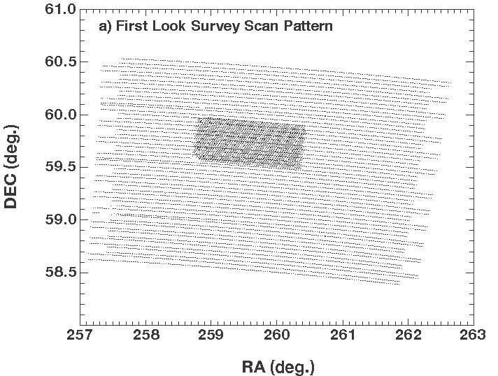
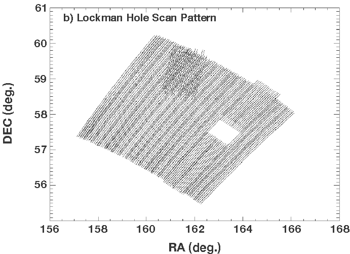
Figure 1: Scan Patterns. A simple representation of the scan pattern, a line connecting each pointing of the camera sequentially, is given above for both fields. Part (a) shows the scan pattern for the First Look Survey (FLS) Extragalactic Field. Note that all scan paths are close to parallel, even those in the verification region (repeated observations denoted by denser region at center). Part (b) shows the Lockman Hole (SLH) Scan Pattern. Note that all scan paths are close to parallel except for those in the validation region (repeated observations denoted by dense region of paths at approximately 45 degrees to nearby paths, at upper middle of figure).

The MIPS camera 160 $\mu$m measurements are made via a stressed Ge:Ga detector array. The response of these detectors is measured frequently using flashes (“stims”) from a light source within the camera at a regular period. Ge detectors are subject to random and 1/f noise components, including gain drift, and “memory” effects, which are extremely difficult to model and correct. (The so-called memory effect refers to detector responsivity changing as a function of the history of flux the detector has been exposed to.) In practice, drift and memory effects are mostly, but not perfectly, corrected. In more typical observations of sources, using scanning or rapid chopping techniques, the rapid appearance and passing of the sources in a given detector pixel limits drift and memory effects to those associated with short time constants. The stims do a good job of tracking the detector response on short time scales, and a standard reduction described in the Spitzer Science Center (SSC) Data Handbook yields excellent results for both point sources and bright extended sources. The MIPS Ge detectors are not optimized for background observations, however. Here long time constant effects (“slow response behavior”) can complicate the reduction and interpretation of the data. Below, we describe modifications to the Data Handbook procedures that we found necessary to obtain good results. Despite that fact that the instrument is not optimized for background observations, we shall demonstrate below that the problems associated with our data are manageable, and a great deal of information is available in these maps.

2.3 Basic Map Reduction

We start with BCD or Basic Calibrated Data from the SSC pipeline reductions (See Gordon et al. 2005 and MIPs Data Handbook). We began our reduction by following the procedures listed in the Data Handbook for reduction of extended sources, but found that modifications were required (described below).

Our co-added maps, which have pixels of the nominal camera pixel size, give the average of the flux measurements closest to each pixel center. No re-sampling of the maps and no distortion corrections have been applied at this time because we are interested in structures much larger than the camera pixel size.

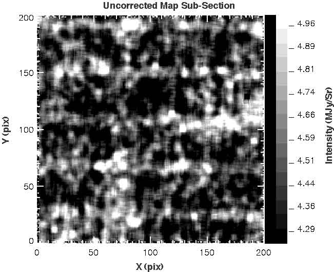
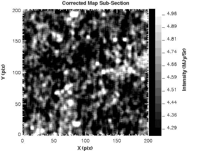
Figure 2: Stim Latent Correction. The two figures show a small sub-section of the co-added SLH map. The top figure shows the uncorrected sub-section, which has regular, bright horizontal bands (perpendicular to the scan direction) which dominate the structure. These bands are due to the stim latent effect. The bottom figure shows the corrected sub-section; the bands have been completely removed by the correction process. The intensity scale (linear, MJy/sr), given at the right side of the figure is the same for both images; the spatial scale markings on the bottom and left sides of the figure are in units of instrumental pixel widths. All data from every field show the same effect. A 5 pixel boxcar smooth has been applied to improve clarity for publication.

Data Selection This work includes data from pipeline version 11, which includes previously embargoed data . Some data covering our selected fields was excluded from our analysis due to data quality or instrument settings. In the SLH maps, a rectangular patch of sky near ($\alpha$,$\delta$) = (163.5^∘, 57.6^∘) is covered in AORs 9632512 and 9832256. These data have high noise and so were not used in our map, leaving a small rectangular region without data, which we refer to as the “window”. These data sets clearly dominated our rms noise map, described below, with a median rms of 0.33 MJy/sr in these regions vs. 0.23 MJy/sr typical of the rest of the map. (The noise also had unusually strong structure in the scan direction.) We also excluded data from PID81, which were taken with different instrument settings (including stim period) and were not appropriate to combine with the rest of our data. Table 2 gives a list of AORs which identify the data used. In the FLS map, all data were used.

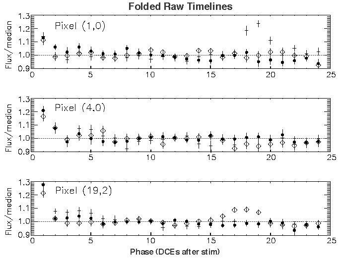
Figure 3: Stim Latents. The data from three different detector pixels are shown folded at the stimulator flash period. To show possible time-dependence of the phenomenon, the first 1/3 of the data were represented by a cross, the second third by a diamond, and the final third by a filled circle. The time bin after the stim flash (which occurs in bin 0 in the figure) is almost always high in almost all channels. (These data are from AOR 5177088.) The variation within an AOR is small compared to the other sources of deviation in the data. The response for a given detector pixel is also consistent between different AORs (with a well-defined average and some variation for different input sky). However, each detector pixel has it’s own characteristic response curve, hence our independent correction for each pixel.

Stim Correction In both “raw” maps (direct co-adds of BCD), obvious parallel bands can be seen perpendicular to the scan pattern (See Fig. 2). These correspond to the frames taken just after the stim flash response measurements; the effect is referred to as a “stim-flash latent”. The stim flash itself necessarily contributes to memory effects in the detectors, as would any illumination. These effects depend on the integrated illumination history, not just the instantaneous brightness. Although the flash is very bright compared to typical source and background fluxes, it is very short in duration, producing small integrated fluence, and so causes only a small memory effect. Unfortunately, the small stim latent is significant compared to the faint CFIB.

Figure 3 shows BCD light curves from the observations of the SLH field at 160 $\mu$m (AOR 5177088) folded at the stim period. Here, each period of data was divided by the median of the data during that period in order to remove variations of the sky level during the observation. As can be seen in the figure, for a given pixel, the behavior is fairly consistent within a single AOR, but individual pixels can be significantly different from each other. Examination of all such response curves among all AORs shows that the behavior follows normal statistical variation expected for varying input sky, with a well-defined average for every time bin for every pixel. We therefore applied a single stim latent correction to all data, but with a separate correction for each pixel. In most pixels, the residual effect is 10% - 20 % in the time bin or DCE after the stim flash, much greater than the error bars from the variation in sky flux (3-5%; see Fig. 3). The correction is simply the inverse of the folded and normalized timelines. A comparison of the sky maps made with and without the stim-flash latent corrections, shown in Fig. 2, is dramatic. The dominant structure in the raw map, the lines made by the stim-flash latents, has been removed.

Illumination correction The Spitzer Data Handbook recommends that an illumination correction be made for extended source observations. We therefore performed corrections similar to those for CCD flat correction. We found the median value for each detector over a large set of data; this median “image” was then normalized, and all data in the sample were then divided by the median image. The standard deviation of the pixel corrections was typically 7%. We tested making a different illumination correction for each scan (i.e. correcting only the data between each change of scan direction, as recommended in the Data Handbook), and also using the same correction for an entire AOR. If an illumination correction were beneficial, we would expect that the rms deviation between repeated measurements of the same sky would decrease. In both cases, no significant decrease in rms deviation was achieved.

2.4 Zero-Point Correction

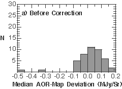
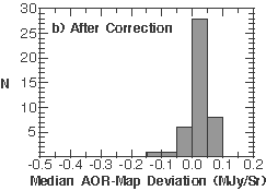
Figure 4: SLH Median AOR Deviation. In part a), above, the histogram of median deviation (median of data $-$ map) for each AOR in the SLH map is shown. The two outliers are 770624 and 770368, the validation region scans ($-$0.34, $-$0.48). In part b), below, on the same horizontal scale, the histogram of residual median deviations is given (i.e. after the optimal set of offsets was added to the data). The added offsets make the distribution much more narrow. The two outlying points are again AORs 770624 and 770368 ($-$0.08, $-$0.11).

In our initial co-added maps, regions associated with a given AOR appeared to have discontinuous flux on the borders of regions covered by other AORs. On further investigation, we found that this was reflected in a systematic discrepancy between measurements of the same sky position during different AORs. This can easily be seen in the histogram of median AOR data-map deviation. (We define the deviation $\delta$_i of each measurement f_i in a given AOR at a sky location r(i) to be the difference between that measurement and the map at the location of the measurement, or $\delta$_i= f_i(r(i)) - map(r(i)). The map value is just the average of all flux measurements f at any given position, map(r(i)) = <f(r(i))>. The median deviation for a given AOR is then D = median($\delta$_i) for all i in the AOR.) The histogram of median AOR deviation is shown in Fig. 4 for our selected data. The obvious outliers in the SLH data are from observations of the “validation region” of the survey. The validation region data were taken 2003 December 9, long before the rest of the survey, 2004 May 4-9. According to the SSC tool SPOT, the level of zodiacal light is estimated to be 0.22 MJy/sr lower during the validation observations. However, the deviation in the other data sets taken at the same time is apparently instrumental in nature.

We used numerical techniques to find the minimum variance (of repeated observations of the same sky pixel) set of additive zero point constants to reduce this problem. The set of minimum variance constants is given in Table 2 for our SLH map. We note that this process changes the zero-point flux of the map (as noted in Table 1); while appropriate for investigations of fluctuations it is not intended for correction of the absolute flux zero-point of a map.

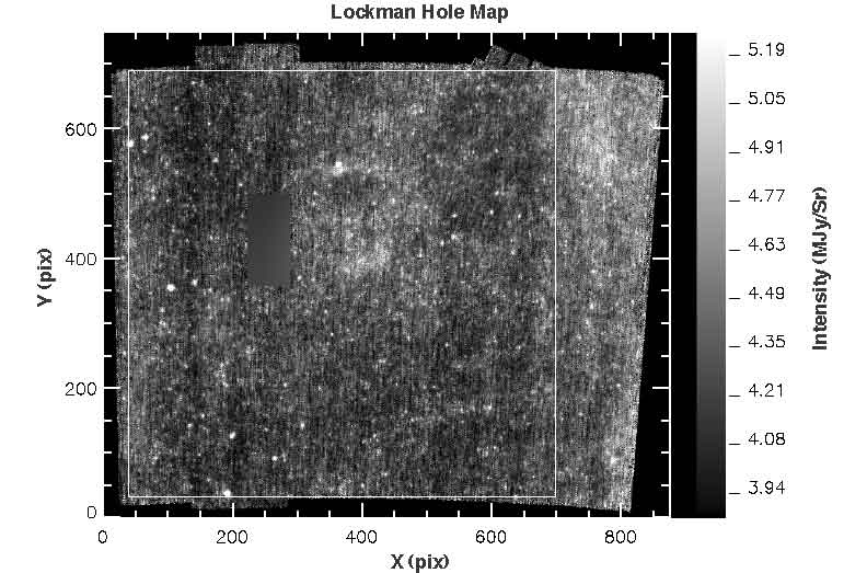
Figure 5: Full SWIRE Lockman Hole (SLH) 160$\mu$m Map (Scan Direction Vertical). The full SLH map is shown above. The small protrusions at the upper right are the edges of the validation region scans, which are roughly 45^∘ from the main scans. The white rectangle indicates the square sub-region used in our analysis. Because of the strong cirrus emission at the right side of the image, this region was omitted from our analysis sub-region. The unnaturally smooth rectangle centered near 250, 425 is the “window” referred to in the text with interpolated data (see text section 3.1). The x and y spatial scales are in pix (15.9”/pix). The bar at right indicates an intensity scale, in MJy/sr. The image is rotated so that the main scans are approximately vertical.

Zodiacal Light No zodiacal light correction was applied (except in the correction for a different observation epoch, as described above); we show in Section 3, Map Power Spectra, that this produces negligible effects on our results.

Figures 5 and 6 show the SLH and FLS maps, respectively, with all the reduction steps described thus far.

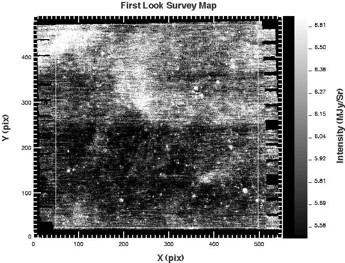
Figure 6: First Look Survey (FLS) Map (Scan Direction Horizontal). The full FLS map is shown above. The verification region, where additional observations were made, is a small region just below center. The same spatial and intensity units are used as in the previous figure. The figure is rotated so that the scans are approximately horizontal. AOR boundary-related structure is evident. The overlap of adjacent regions covered by different AORs is smaller than in the SLH map, and the average number of observations per sky pixel is lower, making good offset corrections particularly challenging. The cirrus flux is also higher. (Because of the poor map quality and high cirrus, this map was not used in our final CFIB spectrum or related conclusions. The white rectangle indicates the sub-section used in the power spectrum of this region shown in Fig. 10. See text for details.)

2.5 Striping

Striping is a common problem in intensity mapping. When a detector is moved on a contiguous path, slow changes in detector response (“drift”) will result in structure in the map related to the scan pattern which looks like stripes. Our maps have such structure. This can be seen clearly on a computer screen, though it often shows up poorly in printed reproductions. The scans are all approximately parallel in the maps (except for small validation regions), enhancing this structure. In Fig. 7 we show the SLH map smoothed at a size of 1/2 the instrument width to emphasize this effect; the figure has been rotated so the scans are vertical, and the structure is also vertical. The structure in the map looks like large blocks, the regions covered by each AOR, rather than thin stripes.

Monotonic drift in most detectors in the array, zero-point offsets in most detectors, and memory effects can contribute to striping. We compared the individual detector timelines to the average of all measurements at the same map points, and determined that there was no significant linear drift in any pixel timeline. Detector memory effects are extremely difficult to test for, however, and the contribution of this effect remains unknown. Detector memory effects can cause bright extended emission regions to appear “smeared” across the map in the scan direction, resembling stripes. When the instrument finishes scanning a region and points to a new one, the detector is usually annealed, and its flux history is “reset”. The background in the new region will reflect the detector’s new history while in that region, which will be different than in surrounding regions; hence the discontinuities at the boundaries of the regions covered in each AOR could be caused by memory effects.

Whatever the cause(s), the residual AOR deviations we showed above (Fig. 4b) measure the lowest order (most likely dominant) effect in the timeline data, a constant-per-AOR offset term that causes stripes. Because no statistically significant linear drift is present in the timeline data in either the individual channels or in their averages during each AOR, we assume the offset-like term dominates the striping effect.

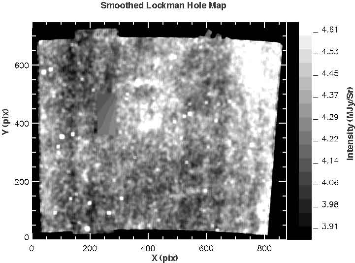
Figure 7: Full Lockman Hole (SLH) Map Smoothed by 1/2 Detector Width (Scan Direction Vertical). This image of the map has been smoothed to enhance structure in the scan direction. Note that in the validation region there is significantly less “smearing” than in the rest of the map due to sampling in different scan directions, i.e. cross-linking. The same spatial and intensity units are used as in the previous figure.

There is one region where significantly less striping occurs in the SLH map, in the validation region (see Fig. 5 and Fig. 7), where some scans were done at large angles to others. (Such scans are said to be “cross-linked”, described below.) Visual inspection of the maps shows the worst striping at the extreme right edge of the map in Fig. 5 and Fig. 7, where several of the brightest, more extended emission regions are located. Much of this region was not included in our power spectrum analysis below, however, due to the known (a priori) high cirrus flux which will tend to dominate the CFIB signal.

3. Power Spectrum Analysis

3.1 Power Spectrum Calculations

Our analysis closely follows that of Lagache et al. (2000). The basic steps for analysis of the CFIB are: (1) A power spectrum is made from the map. (2) Noise is subtracted from the power spectrum, and it is corrected for instrumental response. (3) The local foregrounds are then subtracted to yield the power spectrum of the CFIB. This section will cover all steps of this analysis, and the results will be covered in the following section.

We analyze structure using a simple two-dimensional discrete Fourier Transform on square map sub-sections (shown in Fig. 5 for the SLH map). We report only the average magnitude squared of the Fourier components P(k) in binned k intervals (k =(k_x² +k_y²)^1/2). We did not apodize our maps prior to power spectrum analysis in order to preserve the information in the corners.

In order to measure the noise power spectrum, two separate maps were made from the alternating (i.e. even and odd) measurements at each sky location. The even and odd maps were then subtracted to make a difference map which was analyzed to determine the noise power spectrum.

3.2 Map Preparations

Missing Data Certain artifacts of the maps had to be “repaired” before proceeding to power spectrum analysis. Our SLH field map contains an approximately rectangular section, the “window”, 0.29^∘ $\times$ 0.63^∘ (66 $\times$ 143 pixels) for which all AORs have excessively high noise (see section 2.3). Because the region includes only a small fraction of the map area (0.18 deg², 2.1% of our square map size), the loss of these data should have only a negligible effect on our results. We compared several methods for replacement of the data in this region: replacement with contiguous sections of data taken “above” and “below” the window, from both “sides” of the window, and finally we replaced the data with a smooth fifth order polynomial fit to the data around the window. The power spectrum results were insensitive to the choice of replacement method (or interpolation order), and we finally adopted the smooth fit.

There are unobserved pixels in the maps; in the FLS about 1.3 %, in the SLH 3 $\times$ 10^-4 of the area in our square map was unobserved (in addition to the missing rectangle). We replaced all small groups of unobserved pixels with a local median of non-zero pixel values with a center-to-center distance of $\leq$ 10 pixel widths. These replacements had minimal effect on the final power spectrum.

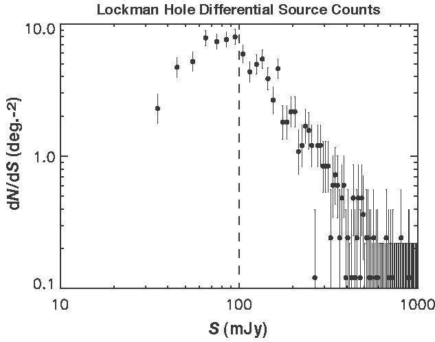
Figure 8: Differential Source Counts for Lockman Hole (SLH) Map. The figure shows differential source counts, dN/dS, where N is the number of sources per unit area, and S is source flux (in uniform 10 mJy bins). We required $S>4\sigma$ for all sources. Error bars give Poisson counting 68% uncertainty. The vertical dashed line indicates the source removal flux cut for our CFIB analysis. (See text for additional details).

Source Removal We removed resolved sources from the maps before CFIB power spectrum analysis in order to remove the contribution of the brightest sources. We used a simple source-finding algorithm and aperture photometry for this goal; for detailed studies of the sources in Spitzer 160 $\mu$m fields, the reader is referred to, e.g., Frayer et al. (2006) and Dole et al. (2004). Source finding can be complicated by the background fluctuations, and following the SSC’s recommended procedure, we found and measured sources in maps made from “median-filtered data”, effectively removing the background before reduction. Here, for each BCD pixel timeline, after applying our stim-latent correction, we then subtracted a median timeline from each pixel timeline. The median timeline was calculated with a moving window 41 DCE in extent. (The “FBCD” median-filtered data from the SSC have the same strong stim residuals as the BCD data, and so were not useable.)

We used the SEXTRACTOR program (Bertin & Arnouts Bertin (1996)) to find source locations (x,y), x and y sizes (s_x, s_y), and fluxes. Aperture and color corrections were not made. Sources with isophotes more than 1.5 $\sigma$ (0.53 MJy/sr) above the local background were considered to be “detected” if they had four or more adjacent pixels above the threshold. The flux distribution of sources with measured fluxes greater than 4 times measurement uncertainty is shown in figure 8.

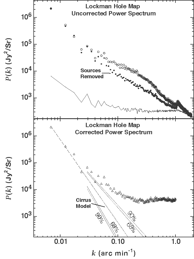
Figure 9: Power Spectrum of Lockman Hole (SLH) Map. In the upper plot, open circles indicate the power spectrum (P(k)) measured directly from the map; filled circles indicate the power spectrum after sources with flux $>$ 100 mJy were removed. The continuous line at the bottom of the figure gives the measured noise spectrum. In the lower plot, drawn on the same scale for comparison, triangles indicate the power spectrum corrected for instrumental response and residual zero-point effects. The power law fit is shown as a dashed line in the range of measurements where the fit is made, and its extrapolation is denoted by a “dot-dash” line (“Cirrus Model”). The dotted lines give the two-parameter 68% (inner set) and 90% (outer set) probability region for the extrapolated cirrus power.

Most of our map has 4 (nominal) MIPS passes over each sky pixel, however, in a small “Validation Region” another 8 passes were made. Not only does this region have significantly longer integration time, the additional passes were made along different directions than the rest of the map data, which is expected to reduce systematics (see section 4.3.2). In order to assess completeness, we compared source detections in this region from maps with and without additional validation data. Sources detected in the “regular + validation data” maps were missed in the “regular data only” maps with systematically increasing frequency below about 90 mJy. We therefore chose 100 mJy as a flux cut value that is relatively conservative in terms of completeness, as well as convenient for comparison to previous measurements. For S $\geq$ 100 mJy, and requiring measurements at greater than 4 sigma significance for detection, 37 sources were detected in the regular data out of 40 sources detected with the additional validation data in the same region. Within the limitation of small number statistics, and assuming the deeper map is 100% complete to 100 mJy, our source lists are greater than 90% complete. This serves as a rough measure of completeness, but note that detection efficiency is expected to vary with local background structure.

A second check on completeness comes from a comparison of our source density with those of other measurements. For our full map, for S$\geq$ 100 mJy, we measure 506 sources for 61.1 sources/$deg^{2}$ ($2.00\times 10^{5}$ sources ${Sr}^{-1}$). This number is midway between the different measurements in Dole et al. (2004), which may be read directly off their figure (see top of Fig. 3 in this work; corrections for completeness were not made), and is also consistent with Frayer et al. (2006).

At the location of each source centroid, a circular region within diameter d_replace was replaced with local background values. The resulting one-dimensional source sizes s = maximum (s_x, s_y), yielded good results as d_replace in the range of 1.5-3.5 times the instrument full width at half maximum, FWHMi (2.375 pix), except for sources with larger measured sizes, which yielded better results when the size was truncated to between 3.5 and 4.5 FWHMi. In the SLH maps only, two very large and bright sources were masked “by hand”. For each pixel in the replacement region, the median of an annulus of inner and outer diameters 3 d_replace and 4 d_replace replaced the pixel value. In the end, the power spectra were insensitive to small variations in d_replace and to a wide range of values of the detection isophote threshold.

Sub-Sample Selection The only significant exclusion in the SLH map was the region at the far right edge in Fig. 5, which was excluded due to high cirrus. With this exception, we analyzed the largest possible square sub-regions of each map (indicated in Figs. 5 and 6). The SLH sub-sample area is 8.47 deg².

3.3 Features of the Raw Power Spectrum

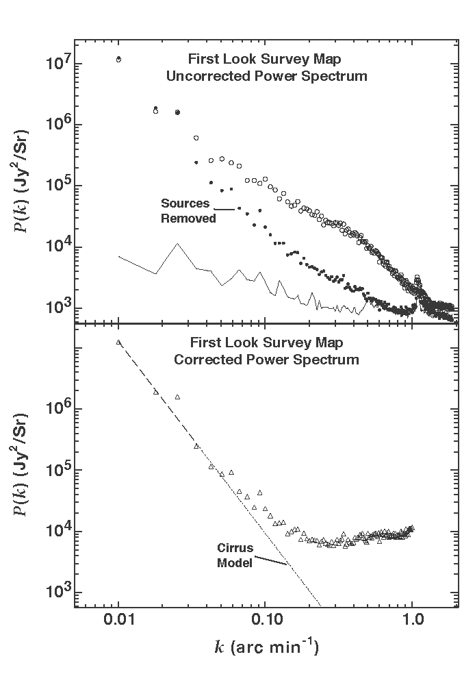
Figure 10: First Look Survey (FLS) Map Power Spectrum. In the upper plot, open circles indicate the power spectrum (P(k)) measured directly from the map; filled circles indicate the power spectrum after sources with flux $>$ 100 mJy were removed. The continuous line at the bottom of the figure gives the measured noise spectrum. In the lower plot, drawn on the same scale for comparison, triangles indicate power corrected for instrumental response (PSF). The power law fit is shown as a dashed line in the range of measurements where the fit is made, and its extrapolation is denoted by a “dot-dash” line (“Cirrus Model”). See text for additional details. Note that the much larger SLH field had measurements down to smaller k (Fig. 9). The power law extrapolation is not much higher than the data up to $\sim 0.09$ arc min^-1, and so the CFIB cannot be measured easily or accurately at low frequency in this field.

The power spectra of the SLH and FLS maps are shown in Fig.s 9 and 10. The following features are of interest: The lowest frequency bins look like a simple power law; in this region IR cirrus emission is known to dominate. In the mid-frequencies, there is excess emission above this power law. This is the signal due to cosmological sources. At the high frequency end, the signal is strongly modulated by the instrumental response function, the power spectrum of the point spread function (PSF) of the instrument and telescope. The power spectrum of the PSF provided by the SSC (simulated by the STINYTIM routine) is shown in Fig. 11. At the highest frequencies, the signal becomes dominated by noise; noise power is within a factor of two of signal by k $\geq$ 0.7 arc min^-1 for the SLH.

3.4 Systematic Effects

Below we list likely sources of systematic errors, and demonstrate that all these errors are small compared to the power spectrum features we are interested in.

3.4.1 Zodiacal Light

The zodiacal light contribution to the power spectrum at 160 $\mu$m is small compared to our CFIB fluctuation signal, and so we did not attempt to remove any zodiacal light signal from our maps prior to analysis. At 160 $\mu$m, a simple, planar fit to the zodiacal background values predicted by SPOT was analyzed to determine the effect on the power spectrum. We estimate that zodiacal light contributes less than 2.5% of the spectral power in any bin, with a maximum contribution at low k.

3.4.2 Stripe Reduction and Residual Stripe Effects

As shown in section 2.4, there are systematic deviations in each AOR data set that have the character of a zero-point offset. Such a set of zero-point offsets might cause false structure because the scan pattern is rather regular. We tested the effects of such offsets on the power spectrum by producing a known, “synthetic sky”, then simulating observation of this “synthetic sky”, including the addition of noise and offsets. Comparison of the known input synthetic sky and the resulting maps will then give the systematic effects due to the zero-point offsets.

We produced our synthetic sky with a very simple Poisson distributed model CFIB + foreground cirrus. We used an actual cirrus image from ISSA plates with point sources removed and re-binned to the same pixel size as in our map. This cirrus foreground image has the desired -3 slope spectrum, but much stronger cirrus than in our field. We scaled this image in intensity such that it had the same low-k cirrus power spectrum amplitude as in our SLH map. We then added a Poisson distributed synthetic CFIB signal (i.e. with a flat power spectrum), such that it produced the same power spectrum amplitude as the flat high-frequency component of the SLH power spectrum. We then simulated scanning observations, using the same scanning pattern as in the SLH observations, adding the measurement noise and offsets as described for the different simulations below.

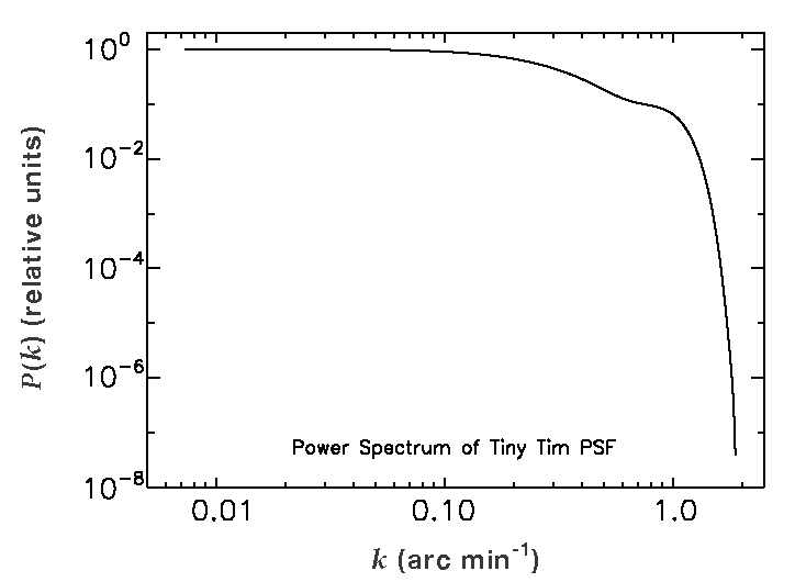
Figure 11: Power Spectrum of PSF. (PSF generated by the routine Stiny Tim.)

Offset Correction Simulation Test: In our first test, we essentially measure the ability of our mapmaking software to correct for offsets given the SLH scan pattern and measured noise. We started with our synthetic sky simulation and added the same noise power as observed in the SLH, and the actual set of median deviations measured in the BCD data. Different realizations of the simulated observations were achieved by adding the set of deviations to the simulated AOR data sets in a different, randomly scrambled order (i.e. a given offset was assigned to a different region on the map), for each realization. (We generated these different realizations in order to understand effects similar to offsets in a very general way.) We reduced the simulated observation data sets in the same way as our real maps, fitting for zero-point offset corrections. At this point, most of the effects of offsets should have been corrected, and we expect little effect on the power spectrum.

Despite realistic added noise, our offset correction routine worked well, yielding small residual deviations. The power spectrum showed only a very small effect due to uncorrected offsets ($<15\%$ for $k<1$ arc min^-1), negligible compared to the uncertainty due to the fit errors at low k.

Residual Offset (Stripe Effects) Simulation and Correction: Here we observe the effects of uncorrected, residual offsets on the power spectrum, to match the offsets seen in Fig. 4b. Starting again from synthetic sky maps, we simulated observing on the SLH scan pattern, added the same random noise power as observed in the SLH, and the same set of residual median deviations measured in our final SLH map (see Fig. 4b). Analogous to the procedure above, different realizations of the simulated observations were achieved by adding the set of residual deviations to the simulated AOR data sets in a different, randomly scrambled order, for each realization. (We generated these different realizations in order to understand effects similar to the measured residual deviations in a very general way.) We reduced these simulations in the same way as our real maps, but of course, without correcting the residual deviations. The effect on the power spectrum is $<25\%$ for $k<1$ arc min^-1 (see Fig. 12). These errors are small compared to uncertainties in the low-k power law fit which dominate the low- to mid-k CFIB measurement, discussed in the next section. Below, we make use of the function in Fig. 12 to make a correction for the effect of residual deviations on the power spectrum, the inverse of the function in the figure.

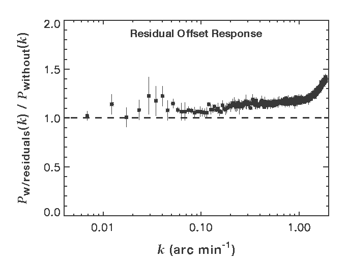
Figure 12: Effect of Residual Offsets on the Power Spectrum. The figure shows the relative effect of the observed residual offsets on the power spectrum. See Section 3.4.2 for details.

3.5 CFIB Analysis

The CFIB analysis requires correction of the raw map power spectrum for potential effects due to offsets and removal of foregrounds.

Instrumental Response Correction The sky map may be described as the convolution of the real sky and an instrumental response function plus noise. The power spectrum of the sky may therefore be derived from the instrumental power spectrum minus the noise power spectrum, divided by the response function of the instrument. In the analysis below, we assume that the PSF dominates the instrumental response function, and approximate our instrumental response function by the power spectrum of the PSF given in Fig. 11.

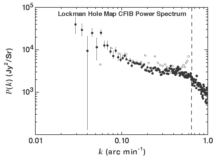
Figure 13: CFIB Spectrum from the SLH (Lockman Hole) Map. The figure shows our noise-subtracted, instrumental response, and residual deviation-corrected CFIB spectrum of the SLH subsample (filled circles). The low-frequency power appears to fall rapidly to $\sim$0.1 arc min^-1; there is a comparatively flat region $\sim$ 0.2 - 0.4 arc min^-1. The error bars give the 68% probability intervals for uncertainty due to the cirrus power law subtraction and residual deviation correction. The cirrus subtraction uncertainty dominates at low frequencies. The diamonds reproduce the results given in Lagache & Puget (LagachePuget00 (2000)). For k $>$ 0.7 arc min^-1 (vertical dashed line) the noise becomes within a factor of 2 of the signal, and the PSF correction is greater than a factor of 10.

Residual Offset Correction to the Power Spectrum We also applied a correction for our residual offsets (measured residual deviations) described in Section 3.4.2. To correct for these residual offsets, we divided out the effect of these offsets in our simulations, the function given in Fig. 12.

Foreground Cirrus Subtraction

Previous measurements of the sky on scales from arc seconds to much larger than our maps have shown that cirrus structure has a power law shape with a log slope very close to –3 (e.g., Wright Wright (1998), Herbstmeier et al. Herbstmeir (1998), Gautier et al. Gautier (1992), Kogut et al. Kogut (1996), Abergel et al. Abergel (1999), Falgarone et al. Falgarone (1998)). This very steep slope means that this structure must dominate at the lowest frequencies (as shown in Fig. 9). Following Lagache et al. (Lagacheetal00 (2000)), we subtract a power law fit of the low-frequency structure from our power spectrum in order to remove the cirrus contribution. We fit a power law function to the lowest four bins of k in order to get a good fit of the cirrus structure in the range of k where it dominates. Unlike Lagache et al. (2000) we do not assume a power law slope, but fit both amplitude and slope. Given the extensive evidence for power law cirrus structure, we decided to empirically determine our fit errors from the deviation in the log of our data from the even-weighted power law fit. The dotted lines shown in the bottom plot of Fig. 9 reflect our mapping of 2-d $\chi^{2}$ space 68% and 90% probability contours. These fit errors dominate the uncertainty in our CFIB measurements at low-k. The resulting CFIB fluctuation power spectrum (the result of subtraction of the cirrus fit from the corrected power spectrum) is shown for the SLH field in Fig. 13. (The upper and lower error bars in the figure are the sum in quadrature of the 68% upper and lower fit uncertainties and the 1 $\sigma$ errors in the residual offset correction.)

4. Results

4.1 The CFIB Fluctuations Measurement

4.1.1 The SLH CFIB Fluctuation Spectrum

The observed CFIB power spectrum is described in gross terms as showing high power at low k, decaying rapidly to $\sim$0.1 arc min^-1, with a relatively flat region $\sim$0.2 - 0.4 arc min^-1. If the sources of the CFIB were distributed at random in space, a flat power spectrum would be expected. What is observed is clearly different. This excess CFIB power at low k has been identified as the signature of clustering of CFIB sources, discussed in the following section. The error bars on the lowest few k values are large due to the finite uncertainty in the subtracted power law fit. However, the remaining points have quite reasonable uncertainties, and we concentrate on these in our discussion. At the large k values, the noise becomes significant and the instrumental correction becomes very large (see Fig. 9; the figure is cut off at k = 1.0 arc min^-1. )

4.1.2 Comparison with Predictions

Perrotta et al. (2003) showed the effects of predicted clustering on background power spectra, using a spiral+starburst population, as did Lagache, Dole & Puget (LDP03 (2003)). Lagache, Dole & Puget (LDP03 (2003)) constructed simulations of Spitzer shallow survey observations, but distributing their galaxy populations at random (without clustering) for comparison. The simulations used a galaxy distribution (“normal” spirals + evolving starburst galaxies) and evolution constructed to be consistent with IR - mm source counts, with sources distributed at random, and interstellar foreground cirrus. By comparing their simulation of cirrus plus unclustered (Poisson distributed) galaxies to the clustering component predicted by Perrotta et al. (2003), they were able to predict that the clustering component would be visible as a bump above the cirrus and Poisson components in the range of k $=$ 0.04 – 0.2 arc min^-1. In Fig. 14 (after Dole, Lagache, & Puget, 2003, Fig. 11) we show the theoretical clustering component prediction, along with power spectrum components from our SLH map, the power law fit to the cirrus, and the flat or “Poisson” component (the average flux density measured from 0.2 arc min^-1 to 0.5 arc min^-1, 3203 MJy/Sr). (Note that Perrotta et al. 2003 remove sources down to 135 mJy from their analysis, not 100 mJy as we do here.) Looking at Fig. 14 and following Dole, Lagache, & Puget (2003), a clustering “signature” should be detectable roughly between $\sim$ 0.03 and 0.3 arc min^-1, where the clustering power spectrum component is greater than the cirrus and “Poisson” components.

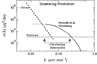
Figure 14: Power Spectrum Clustering Prediction. The power spectrum figure above shows the Perrotta et al. (2003) clustering prediction (for sources with fluxes $<$ 135 mJy; short dash line) taken from Dole, Lagache, & Puget (2003). We also show our Poisson level from the SLH map power spectrum (the average power measured between k $=$ 0.2 and 0.5 arc min^-1, 3203 MJy/Sr; solid line). The cirrus foreground structure fit from the SLH map is also shown (longer dashed line). Following Dole, Lagache, & Puget (2003) a clustering “signature” should be detectable between roughly k $=$ 0.03 and 0.3 arc min^-1. We see an excess in our SLH map power spectrum in about the same range, k $\sim$ 0.03 to 0.15 arc min^-1 (Fig. 13).

In the grossest sense, these predictions do agree with our CFIB spectrum, in that there is a substantial low-to-mid k excess above a relatively flat high- k “Poisson” region, the clustering “signature”, clearly inconsistent with a Poisson distribution of sources. In detail, however, Perrotta et al. (2003) predicts that the power spectrum excess is almost flat for k in the range of 0.01 to 0.1 arc min^-1, which is not consistent with our observations. Our points with small error bars near k $=$ 0.045 and 0.06 arc min^-1 require a drop of greater than a factor of 3 in power between these bins and 0.1 arc min^-1.

4.1.3 Impact of Systematic Effects

These results are from a relatively simple analysis which explicitly assumes that the SSC PSF simulation gives the correct instrumental response function. However, it is extremely unlikely that an instrumental feature would produce our excess low-k (large-scale) power. Large and medium scale power in the instrumental response function can only come from changes in the instrument over times comparable to observation of the whole map; the camera PSF has no structure on large scales (see Fig. psfpowspec). The map was sampled rather uniformly on the large scales, with essentially the same scanning overlap, redundancy, scan speed, etc. across most of the map. There is no strong feature in the power spectrum (except for the high-k PSF signature) common to any set of maps we have examined that would suggest a significant uncorrected instrumental artifact. The ISO instrument (Lagache & Puget LagachePuget00 (2000)) also had no features in the instrumental response in the low- to medium-k range, and in general, such features would not be expected. We note that the excess clearly extends into the mid-k region (the power is more than a factor of two above the flat region all the way up to k $=$ 0.08 arc min^-1). The map contains many samples of the associated size for mid- k values, therefore the measured behavior cannot be a statistical anomaly. We also note that spurious artifacts generally occur at much smaller spatial scales.

In section 3.4.2 we addressed the possibility that systematics with the character of an instrumental zero-point offset could cause erroneous structure in our power spectra. The result of our simulations showed that after we corrected for offsets, this was a small effect. (Compare the magnitude of the excess in Fig. 13 to the magnitude of the corrections in Fig. 12.) Further, we applied a correction to the spectrum for the residual uncorrected offsets (stripes). The consistency of our simulations makes us confident in this correction. In the end, however, the erroneous structure and correction had little effect on the results. Table 3 lists the power law fits to the SLH power spectrum with and without offset and residual spectral corrections, and they are essentially indistinguishable. Because the dominant error in the CFIB spectrum is the power law subtraction uncertainty at the low to mid-k points of interest, and because the power law fit did not change, neither the effect of the offsets nor the corrections significantly changed the results in the low to mid-k points of interest. The excess at low to mid-k is simply larger than any of these effects or corrections. Our main result of excess power at low to mid-k is therefore robust against such systematic effects, within our errors.

Table 3: Low-k Power Law Slopes

Map and Sample	Cirrus Power Law Slope
SLH,corrected	–3.11 $\pm$ 0.30
SLH,uncorrected	–3.09 $\pm$ 0.29
FLS	–3.12 $\pm$ 0.55

4.1.4 Dispersion in the SLH Results

The SLH sub-sample was selected in order to avoid bright cirrus regions and map edges. We reduced a few different sub-sample regions of similar size within the full map (Fig. 5) which included varying amounts of bright cirrus. As the subsample included more bright cirrus, we found larger uncertainties in the power law fits and associated larger CFIB power spectrum errors. All cirrus-subtracted CFIB power spectra are consistent within errors, however.

We note that the two SLH validation AORs yielded the largest deviation even after zero-point correction (Fig. 4). Removal of these two AORs from the map yielded results consistent with those reported above. Because we did not find otherwise obviously anomalous behavior in the region covered by these data in the difference maps, however, we judged that elimination of these data may not be justified. We therefore did not eliminate these data.

4.1.5 First Look Survey Results

The FLS map power spectrum has no obvious turn-off from the cirrus power law until about 0.09 arc min^-1, whereas in the SLH power spectrum, the turnoff was at $\sim$ 0.03 arc min^-1. The difference is due to the greater strength of the cirrus emission in the FLS field. The cirrus power is more than 10 times higher in the FLS at 10^-2 arc min^-1 than in the SLH.

The power law fit was again made from the first four bins. However, the field is smaller, so the first four bins are at higher frequency than in the SLH. In this field, the power law fit has larger uncertainty than in the SLH. Because of this larger uncertainty, the signal in the low to mid-k range of interest has large error bars, and the resulting CFIB measurement is not interesting. This result is not unexpected, however: the combination of strong cirrus in the field (requiring very small fit error for CFIB measurement), and sampling the cirrus at a higher k (because the field is smaller) where the CFIB can interfere makes for an a priori difficult measurement.

Table 4: Power Spectra Compared

	This Work					Other Work
Scut	P0.2-0.5a	P0.05-0.5b	Measurement	PPoissonc	Measurement	PPoissonc	Measurement	PPoissonc
(mJy)	(Jy2/sr)	(Jy2/sr)		(Jy2/sr)		(Jy2/sr)		(Jy2/sr)
250	3920	5341	ISO Lockmand	12000$\pm$ 2000
100	3203	4472	ISO Maranoe	7400	ISO ELAIS N1f	5000	ISO ELAIS N2f	5000

aAverage, even weight per bin, over the relatively flat region of our spectrum, k $=$ 0.2-0.5 arc min-1.

bAverage, even weight per bin, k $=$ over 0.05-0.5 arc min-1.

cResult of Poisson sources + Cirrus Fit.

dMatsuhara et al. (Matsuhara (2000))

eLagache & Puget (LagachePuget00 (2000))

fLagache et al.(Lagacheetal00 (2000))

4.2 Comparison with Previous Results

Background Level The SSC provides a tool to separately predict the local, ISM, and extragalactic background components (part of the SPOT software) incorporating HI data and IR measurements (essentially the Schlegel, Finkbeiner & Davis (Schlegel (1998)) results), and knowledge of the MIPS instrument. Table 1 shows that in all cases, the median total background is much higher than the prediction. It turns out that there is a known, but undocumented, constant zero-point flux offset of about 1 MJy/Sr in the MIPS 160 camera, in all modes, essentially an uncorrected dark signal (Noriega-Crespo Noriega-Crespo (2006)). Subtracting the 1 MJy/Sr offset would greatly improve the agreement between the SPOT predictions and the measurements. The SPOT predictions do agree roughly with measurements from other instruments in this wavelength regime (e.g. ISO measurements in the FIRBACK fields; Lagache & Dole 2001), however the predictions are not intended to be precise and in particular suffer the limitation of not including CFIB fluctuations.

CFIB Fluctuations The Lagache et al. (Lagacheetal00 (2000)) ISO CFIB fluctuation spectrum results for the ELAIS N2 field at 170 $\mu$m (diamond symbols), with the same 100 mJy source removal, are plotted along with our results in Fig. 13. (The values were taken directly from their Fig. 3.) The Lagache et al. (Lagacheetal00 (2000)) values are systematically higher ($\sim$ 35% higher in the mid-k region), but given the bin-to-bin scatter, differences in instruments, and realistic measurement and calibration uncertainties, the agreement is as good as can be expected. We note that the Lagache et al. (Lagacheetal00 (2000)) values are consistent with the same systematic rise toward low-k as is seen in our measurements.

Most other works do not give a cirrus-subtracted CFIB spectrum; they only report an effective average power spectrum value, so comparisons are less straightforward. All the other authors assumed the CFIB power spectrum to be flat, which we have shown is incorrect. (The average power spectrum value is then dependent on the range of k over which the average is taken, and even possibly on binning.) In Table 4, we give average values from our SLH map spectrum, as well as other published measurements. Our “Poisson level” values, which we putatively identify with the relatively flat region k = 0.2-0.5 arc min^-1, are much lower than any of the other values in the table. We also report, however, an average power over a larger range in k, 0.05-0.5 arc min^-1. This range in k is closer to that used in the fits of the other authors, and gives closer results. The disagreement with Matsuhara et al. (Matsuhara (2000)) in the same region of the sky, however, is large. Such a large difference is likely due to different flux calibrations. For the measurements with source removal down to 100 mJy, the agreement is better; our 0.05-0.5 arc min^-1 value is only 11% below the values given by Lagache et. al (Lagacheetal00 (2000)) for the ELAIS fields, though $\sim$ 30% below the value for the Marano field (Lagache & Puget LagachePuget00 (2000)). None of these works, however, claims to have addressed the background flux calibration uncertainties of their measurements. In our case, the MIPS flux calibration continues to evolve, and is a likely source of disagreement with other instruments.

5. Discussion

5.1 Measurement of Clustering

As noted in the introduction, one may convert structure found in optical correlation function measurements to an intensity fluctuation angular power spectrum. The result is a power law excess at low-k due to clustering, falling to a flat Poisson component at some higher k. The Perrotta et al. (2003) prediction, explicitly for the 170 $\mu$m CFIB fluctuation power spectrum, also predicts a low-k excess due to clustering. In gross detail, this is what is observed, and is therefore no surprise. This detection of clustering structure is also robust because the systematics have been explicitly controlled: first, our simulations show that there can be no significant low-frequency distortions in the power spectrum due to offset-like effects, and second, because PSF and other instrumental corrections are small at low-k.

Now let us consider the shape of the CFIB power spectrum in more detail. Though our results are similar to the power spectrum predicted by Perrotta et al. (2003), in detail our results are clearly different. The steeply descending low-k spectrum we observe would be very difficult to fit to the nearly flat excess predicted by Perrotta et al. (2003) in this region. This predicted flatness comes from the details of the population model used for the prediction: At low k the Perrotta et al. (2003) power spectrum is dominated by the contribution from starburst galaxies, which is a nearly flat for k $<$ 0.1 arc min^-1. This prediction has spiral galaxies, contrarily, having a power spectrum contribution that falls steeply with k, precisely what is required to reproduce our sharply falling spectrum at low k. If the power spectrum contributions of the two galaxy types were correct in shape but not in strength, then the contribution of spirals would need to be much larger than that in Perrotta et al. (2003), about a factor of 7 larger. (We made a crude fit of the Perrotta et al. 2003 spiral contribution to our low-k data, taking the power spectrum values from their Fig. 7, and determined that the spiral contribution would need to be 7 $\pm$ 2 times as great to be consistent with our data. We fit in the range of k $=$ 0.07 to 0.1 arc min^-1.)

The Perrotta et al. (2003) paper has some limitations for comparison in detail to the results here. Their analysis specifies sources removed down to 135 mJy, slightly different than our cut at 100 mJy. The model galaxy distribution used in the prediction is also not consistent with the most recent Spitzer results. For example, their model predicts 3.9 $\times$ 10⁵ sources per square degree at 50 mJy at 175 $\mu$m, which is in poor agreement with the MIPS 160 $\mu$m measurement of (8.5 $\pm$ 1.4) $\times$ 10⁵ sources per square degree (Dole et al. 2004; the uncertainty is the standard deviation of the two values measured on different fields). The log slope of N($>$S) in this region is –2.3 in Perrotta et al. (2003); the measurements from Dole et al. (2004) have a slope of –2.0. On the other hand, the phenomenological galaxy population model of Lagache et al. (2004), which has been updated to be consistent with the more recent MIPS results, is similar in its fundamentals, i.e. starburst galaxies make up the bulk of the contribution to CFIB fluctuations and passively evolving spirals contribute most of the remainder. The power spectrum prediction for this updated model is not given, however, so we do not know how this compares to our results. Future work, including the following, would be a clear way forward to finding the point of model-data discrepancy, and further refinements in our understanding: (i) calculation of the power spectrum with the newest model (incorporating Spitzer data), (ii) testing the model source distribution against the actual source distributions in the deepest MIPS far-IR surveys, for each identified source type, and (iii) using those identified source types to determine relative bias (both directly with the identified sources within the survey, and indirectly by associating a source type with the color classifications in optical surveys). With information on source distributions to a much lower flux, with a power spectrum calculation based on an updated model, with detailed comparisons to optical data, we will be able to better constrain the galaxy population models; adding to all these constraints the structure measurements herein will then realize the opportunity to more precisely measure the structure.

The study of structure in the distribution of IR galaxies has important potential for illuminating the processes that have taken place since the CMB era. A valuable feature of these far-IR measurements is their virtual immunity to extinction and any extinction-related bias (unlike optical galaxy structure measurements). Additionally, current models suggest that the source population that contributes the majority of the power spectrum structure signal is very simple - only starbursts and IR-bright spirals contribute significantly. If these models are correct, this would also reduce problems of source-type bias that are present in some optical studies. Continued refinement of these measurements, and our knowledge of the source populations, will yield a useful new view of structure very much complimentary to that given by optical measurements.

5.2 Possibilities for Future Improvements

We have corrected most of the scan-pattern related structure, and we have shown that the residual scan-pattern related structure in the power spectrum is small compared to the structure we have measured. However, some residual scan-pattern related structure is still present in the map, and this is the first item we would like to improve on in future work. In terms of data reduction, various frequency space filtering methods for removing stripes seem promising, and have been demonstrated on other types of maps (see, e.g., Miville-Deschênes & Lagache Deschenes05 (2005)). In addition, various algorithms are available for optimum statistical weighting of map data to reduce map deviation. We found, however, that unless the deviation in the maps are significantly reduced, these algorithms do not produce good results on these data.

We find that the greatest potential for improving these measurements is in acquiring new data on the SLH field in a manner appropriate for background observations. The MIPS observations are truly exceptional compared to typical background observations in the degree to which “cross-linking” scans were avoided. Virtually all cosmic microwave/mm background experiments incorporate cross-linking in their scanning strategy. Such a strategy causes each sky pixel to be re-sampled along significantly different scanning paths on the sky. A simplified example of cross-linking scans would be a series of two rectilinear raster maps of a region oriented at 90^∘ to each other. Two sky positions measured along the same scan across the first map would be measured on different scans in the second map. Comparison of repeated observations on the same and different scans allows identification and measurement of any systematics that affect the measurements differently on the same and different scans. In the general case, this technique allows inter-comparison of measurements made close together in time (i.e. on the same scan) with those made at much longer time scales. In our case, this comparison would more clearly identify and more accurately measure the zero-point offsets. In all of the large MIPS surveys, rectangular regions of the sky were observed during each AOR, and then immediately repeated on almost precisely the same path (with only minor exceptions). The rectangular regions were oriented very nearly parallel, no scans were made along significantly different directions (except in the very limited verification observations), and these regions had only small edge overlap. Cross-linking was essentially minimized in the existing surveys, permitting inter-comparison among only a small fraction of data measured on different paths in different AORs. It seems clear that if cross-linking MIPS scans were added to existing Spitzer survey regions, significant improvement in the background fluctuation measurement would result. We proposed a program of 10 hours of MIPS observations to make cross-linking scans on this same field during Spitzer Cycle 3. We are confident that the resulting improvement in systematic error will lead to significantly smaller errors in the low-k region of interest, putting even more pressure on the galaxy population models, and contributing to our measurement of structure in the universe as traced by far-IR emitting galaxies. Ultimately we intend that these improved measurements will contribute to guiding our understanding of the physics of formation of structure in galaxies, allowing us to understand the behavior of luminous matter from the CMB era to today.

Conclusions

In this paper we presented co-added maps from two large Spitzer survey fields observed with the 160 $\mu$m MIPS array. Instrumental artifacts, and artifacts related to the scan pattern (i.e. stripes) were observed, but these effects were controlled in two ways: First, the artifacts were substantially reduced by numerically calculated corrections. Second, we carefully measured the errors due to these artifacts by simulation: We added artifacts, at the same intensity measured in the real data, to simulated timeline data, and after the same reduction as for the real data, we compared the resulting power spectra to that expected. In the end, the errors introduced into our CFIB power spectrum were shown to have no significant effects on our conclusions. We measured a cirrus power law slope of –3.11 $\pm$ 0.30 in the SLH field. Subtracting this power law yielded a CFIB spectrum dropping rapidly from k $\sim$ 0.03 arc min^-1, to k = 0.1 - 0.2 arc min^-1, and a flatter region at higher k. Any assumption of a power law cirrus component plus a flat power spectrum from the ensemble of sources, i.e. from a random distribution of sources, is inconsistent with our observations. Our results are consistent with the general characteristics of predictions of a clustering “signature” in the CFIB power spectrum, but are steeper at low-k than some predictions. This is the first reported measurement of clustering derived from far-IR (50-200 ${\mu}$m) observations.

- (1) Abergel A., Andr P., Bacmann A., et al., 1999, in: The Universe as seen by ISO. ESA-SP 427
- (2) Bertin, E., & Arnouts, S. 1996, A&AS, 117, 393
- (3) Connolley, A. J,. et al. 2002, ApJ 579, 42
- (4) Dole, H., et al. 2004, ApJS 154, 87
- (5) Dole, H., Lagache, G., & Puget, J.-L. 2003, ApJ 585,617
- (6) Falgarone E., 1998, in: Guiderdoni B., Kembhavi A. (eds.) Starbursts: Triggers, Nature and Evolution. Les Houches School
- (7) Frayer, D. T., et al. 2006, AJ 131, 250
- (8) Gautier T.N.III, Boulanger F., Perault M., Puget J.L., 1992, AJ 103, 1313
- (9) Gordon, K. et al. 2005, PASP 117,503
- (10) Herbstmeier U., Abraham P., Lemke D., et al., 1998, A&A 332, 739
- (11) Kogut A., Banday A. J., Bennett C. L., et al., 1996, ApJ 460, 1
- (12) Lagache, G. & Puget, J.-L. 2000, A&A 357, 5
- (13) Lagache, G., et al. 2000, “The Extragalactic Background and Its Fluctuations in the Far-Infrared Wavelengths”, in “ISO Surveys of a Dusty Universe”, Proceedings Ringberg Workshop, (Eds.) D. Lemke, M. Stickel, K. Wilke, Lecture Notes in Physics 548 (2000)
- (14) Lagache, G. & Dole, H. 2001, A&A 372, 702
- (15) Lagache, G., Dole, H., & Puget, J.-L. 2003, MNRAS 338, 555
- (16) Lagache, G., et al. 2004, ApJS 154, 112
- (17) Matsuhara, H., et al. 2000, A&A 361,407
- (18) Miville-Deschênes, M. A., & Lagache, G., 2005, ApJS, 157, 302
- (19) Miville-Deschênes, M. A., Lagache, G., Puget, J.-L. 2002, A&A, 393, 749
- (20) Noriega-Crespo, A., 2006, August 10, private email communication.
- (21) Perrotta, F. et al. 2003, MNRAS 338,623
- (22) Rieke, G., et al. 2004, ApJS 154, 25
- (23) Schlegel D. J., Finkbeiner D. P., Davis M., 1998, ApJ 500, 525
- (24) Wright E.L., 1998, ApJ 496, 1