Close Galaxy Counts as a Probe of Hierarchical Structure Formation

Abstract

Standard $\Lambda$CDM predicts that the major merger rate of galaxy-size dark matter halos rises rapidly with increasing redshift. The average number of close companions per galaxy, ${\rm N_{c}}$ is often used to infer the galaxy merger rate. Recent observational studies suggest that ${\rm N_{c}}$ evolves very little with redshift, in apparent conflict with theoretical expectations for the merger rate of dark matter halos. We use a ”hybrid” N-body simulation plus analytic substructure model to build theoretical galaxy catalogs and measure ${\rm N_{c}}$ in the same way that it is measured in observed galaxy samples. When we identify dark matter subhalos with galaxies, we show that the observed lack of close pair count evolution arises naturally. This unexpected result is caused by the fact that there are multiple subhalos (galaxies) per host dark matter halo, and observed pairs tend to reside in massive halos that contain several galaxies. There are fewer massive host halos at early times and this dearth of galaxy groups at high redshift compensates for the fact that the merger rate per host halo is higher in the past. We compare our results to $z\sim 1$ DEEP2 data and to $z\sim 0$ data that we have compiled from the SSRS2 and the UZC redshift surveys. The observed close companion counts match our simulation predictions well, provided that we assume a monotonic mapping between galaxy luminosity and the maximum circular velocity of each subhalo in our catalogs at the time when it was first accreted onto its host halo. This strongly suggests that satellite galaxies are significantly more resilient to mass loss than are dissipationless dark matter subhalos. Finally, we argue that while ${\rm N_{c}}$ does not provide a direct measure of the merger rate of host dark matter halos, it offers a powerful means to constrain both the Halo Occupation Distribution and the spatial distribution of galaxies within dark matter halos. Interpreted in this way, close pair counts provide a useful test of galaxy formation processes on $\sim$10-100 kpc scales.

1. Introduction

Close pairs of galaxies have provided an important empirical platform for evaluating theories of galaxy and structure formation since the early studies of Holmberg (1937). Within the modern, hierarchical picture of cosmological structure formation, galaxy mergers are expected to be relatively common (e.g. Blumenthal et al., 1984; Lacey & Cole, 1993; Kolatt et al., 1999; Gottlöber et al., 2001; Maller et al., 2005) and the enumeration of close galaxy pairs or morphologically disturbed systems has long been used to probe the galaxy merger rate (Zepf & Koo, 1989; Burkey et al., 1994; Carlberg et al., 1994; Woods et al., 1995; Yee & Ellingson, 1995; Patton et al., 1997; Neuschaefer et al., 1997; Carlberg et al., 2000; Le Fèvre et al., 2000; Patton et al., 2002; Conselice et al., 2003; Bundy et al., 2004; Masjedi et al., 2005; Bell et al., 2006; Lotz et al., 2006). Comparisons of this kind are clearly important, as observed correlations between galaxy characteristics and their environments suggest that interactions play an essential role in setting many galaxy properties (e.g. Toomre & Toomre, 1972; Larson & Tinsley, 1978; Dressler, 1980; Postman & Geller, 1984; Barton et al., 2000; Barton Gillespie et al., 2003).

While traditional merger rate estimates have provided empirical tests of general aspects of the formation of galaxies, they have been less useful in testing specific models of galaxy formation or in constraining the background cosmological model. One of the primary difficulties lies in connecting theoretical predictions with observational data. For example, the standard approach uses the observed close-pair count (or similarly, an observed morphologically-disturbed galaxy count) to derive a merger rate through approximate merger timescale arguments. This inferred merger rate is then compared to theoretical expectations for field dark matter halo merger rates, which themselves are quite sensitive to the precise masses and mass ratios of halos under consideration ( see Maller et al., 2005; Bell et al., 2006, for a discussion of predicted galaxy merger rates). In this paper we exploit the information contained in close-companion counts by adopting a qualitatively different approach. We use a “hybrid” analytic plus numerical $N$-body model to predict close-companion counts directly and to compare these predictions with observed companion counts. Encouragingly, the results from this method reproduce observed trends with redshift and number density in galaxy companion counts. More generally, our results suggest that while close companion counts are only indirectly related to dark matter halo merger rates, they may be used directly to constrain the number of galaxy pairs per host dark matter halo. In this way, companion counts provide an important general constraint on the occupation of halos by galaxies and, thereby, on galaxy formation models.

In the context of the standard, hierarchical paradigm ($\Lambda$CDM ), the merger rates of distinct dark matter halos can be predicted robustly. In particular, several studies have demonstrated that the predicted rate of major mergers of galaxy-sized cold dark matter halos increases with redshift as $(1+z)^{m}$, where the exponent lies in the range $2.5\lower 2.58334pt\vbox{\hbox{$\buildrel\textstyle<\over{\sim}\ $}}m\lower 2.58334pt\vbox{\hbox{$\buildrel\textstyle<\over{\sim}\ $}}3.5$ (e.g. Governato et al., 1999; Gottlöber et al., 2001). Naïvely, one might expect that the fraction of galaxies with close companions (or the fraction that is morphologically identified to be interacting) should increase with redshift according to a similar scaling. As we discuss below, the connection between merger rates and the redshift dependence of close companion counts is not so straightforward.

Observational analyses using very different techniques to measure the redshift evolution in the fraction of galaxies in pairs yield a very broad range of evolutionary exponents, $m\simeq 0-4$ (e.g., Carlberg et al., 2000; Le Fèvre et al., 2000; Patton et al., 2002; Conselice et al., 2003; Bundy et al., 2004). With the exception of the Second Southern Sky Redshift Survey (SSRS2) at low redshift (Patton et al., 2000), these measurements use incomplete redshift surveys that are often deficient in close pairs because of mechanical spectrograph constraints. Thus, apparent discrepancies in these studies may result from differing definitions of the pair fraction, cosmic variance, survey size and selection, and survey completeness.

One of the most recent explorations of the redshift evolution of close-companion counts was performed by the Deep Extragalactic Evolutionary Probe 2 (DEEP2) team (Lin et al., 2004), who reported surprisingly weak evolution in the pair fraction of galaxies out to $z\sim 1.1$. In particular, they reported that the average number of companions per galaxy, $N_{c}$, grew with redshift as $N_{c}\propto(1+z)^{m}$, where $m=0.51\pm 0.28$. At face value, this weak evolution seems to be in drastic conflict with the strong, $m\sim 3$ evolution predicted for dark matter halos. Other recent analyses using different data sets and different techniques yield similarly “weak” evolution (e.g. Bell et al., 2006; Lotz et al., 2006).

The resolution of this apparent conflict involves the difference between distinct halos and subhalos. The “predicted” merger rate of $m\sim 3$ applies only to distinct dark matter halos. The prediction for galaxies, on the other hand, is more complicated. Distinct halos are predicted to contain $\sim 10\%$ of their mass in self-bound substructures known as dark matter subhalos (e.g. Klypin et al., 1999). These subhalos are the natural sites for satellite galaxies around luminous central objects. Subhalos can orbit within their host halo for a time that depends on the satellite-to-host mass ratio and on specific orbital parameters, and can appear as close companions in projection without necessarily signaling an imminent galaxy-galaxy merger. Beyond this, precise predictions for the merger rates of galaxies are sensitive to the poorly -understood process of galaxy formation inside dark matter halos. In work that is based on dissipationless cosmological simulations, galaxy formation unknowns can be absorbed into various prescriptions for assigning observable galaxies to dark matter halos and subhalos (for related discussions see, e.g., Klypin et al., 1999; Bullock et al., 2000; Diemand et al., 2004; Gao et al., 2004; Nagai & Kravtsov, 2005; Conroy et al., 2006; Faltenbacher & Diemand, 2006; Wang et al., 2006; Weinberg et al., 2006).

In this work we use a large cosmological N-body simulation to calculate the background dark matter halo distribution and an analytic formalism to predict the subhalo populations within each of these host halos. There are several noteworthy advantages to adopting this approach. First, we rely on straightforward mappings between galaxies and dark matter halos and subhalos. Second, we measure the average number of close companions, $N_{c}$, in our simulations in exactly the same way in which they are observed in the real universe. We then use the observed companion counts directly, rather than inferred merger rates, to discriminate between simple and physically-reasonable scenarios for associating dark matter halos and subhalos with luminous galaxies. Our approach also allows us to overcome several technical issues. Using analytic models with no inherent resolution limits to model substructure allows us to overcome possible issues of numerical overmerging in the very dense environments (e.g., Klypin et al., 1999) where close galaxy pairs are often found. Furthermore, our analytic subhalo model allows us to assess the variance in close-companion counts that can be associated with the variation in substructure populations with fixed large-scale structure. Our methods also allow us to test for the importance of cosmic variance and chance projections. We find these effects to be small for typical close companion criteria at redshifts less than $z\simeq 2$ in our preferred model.

A powerful way to quantify and parameterize the way in which close pairs constrain the relationship between halos and galaxies is through the halo occupation distribution (HOD) of galaxies within dark matter halos. The HOD is the probability that a distinct, host halo of mass $M$ contains $N$ observed galaxies, $P(N|M)$, and is usually parameterized in a simple, yet physically-motivated way (e.g., Berlind & Weinberg 2001, Kravtsov et al. 2004a and references therein). Coupling the HOD with a prescription for the spatial distribution of galaxies within their host halos allows for an approximate, analytic calculation of close pair statistics (Bullock, Wechsler, & Somerville, 2002). Using pair counts to constrain the HOD and the distribution of galaxies within halos provides a direct means to separate secure cosmological predictions for dark matter halo counts from uncertainties in the more complicated physics operating on the scales of individual halos and subhalos (e.g., star formation triggers and orbital evolution). As we discuss in § 4, the HOD methodology also provides a useful physical platform for interpreting our specific simulation results and for extending them to provide a general constraint on galaxy formation models.

The outline of this paper is as follows. In § 2, we outline our methods, discuss our simulations, and investigate the importance of interlopers in common estimators of the close pair fraction. We present our predictions for the companion fraction, $N_{c}$, in § 3 and investigate its dependence on galaxy number density and redshift. We compare our general model predictions to the observed evolution in $N_{c}$ with redshift in § 3.1 and with our own analysis of pair counts from the UZC redshift survey and SSRS2 at $z=0$ in § 3.2. We discuss the importance of cosmic variance in pair analyses in §3.3 and provide general predictions for future surveys in § 3.4. In § 4 we present a detailed discussion of our results in the context of the galaxy HOD, and explain the predicted evolution in pair counts as a consequence of the convolution of a halo merger rate that increases with redshift and a halo mass function that decreases with redshift. We conclude in § 5 with a summary of our primary results and a discussion of future directions.

2. Methods

The following subsections detail our theoretical methods. Briefly, we investigate pair count statistics using an $N$-body simulation to account for large-scale structure and the host dark matter halo population as described in § 2.1. We use an analytic substructure model (Zentner et al., 2005) to identify satellite galaxies within these host halos as described in § 2.2. This “hybrid” technique overcomes difficulties associated with numerical overmerging on small scales in the large cosmological simulation box and has already been demonstrated to model accurately the two-point clustering statistics of halos and subhalos (Zentner et al., 2005). We use a simple method to embed galaxies in our simulation volume (§ 2.3) and “observe” these mock galaxy catalogs in a manner similar to those used in observational studies. We then compute pair fraction statistics that mimic those applied to observational samples (2.4).

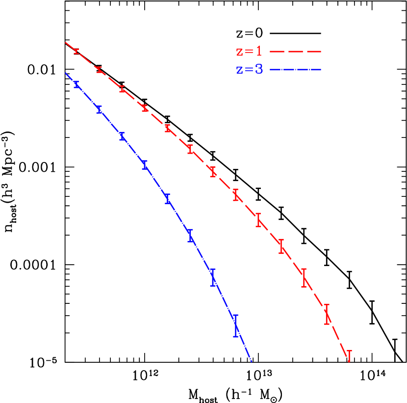
Figure 1.— The cumulative mass function of host halos as derived from our $120$ $h^{-1}{\rm Mpc}$ simulation box at $z=0$, $1$, and $3$. Error bars estimate cosmic variance using jackknife errors from the eight octants of the computational volume.

2.1. Numerical Simulation

Our simulation was performed using the Adaptive Refinement Tree (ART) $N$-body code (Kravtsov et al., 1997) for a flat Universe with $\Omega_{m}=1-\Omega_{\Lambda}=0.3$, $h=0.7$, and $\sigma_{8}=0.9$. The simulation followed the evolution of $512^{3}$ particles in comoving box of $120h^{-1}{\rm Mpc}$ on a side and has been previously discussed in Allgood et al. (2006) and Wechsler et al. (2006). The corresponding particle mass is $m_{p}\simeq 1.07\times 10^{9}h^{-1}M_{\odot}$. The root computational grid was comprised of $512^{3}$ cells and was adaptively refined according to the evolving local density field to a maximum of $8$ levels. This results in peak spatial resolution of $h_{\mathrm{peak}}\simeq 1.8h^{-1}{\rm kpc}$ in comoving units.

We identify host halos using a variant of the Bound Density Maxima algorithm (BDM, Klypin et al., 1999). Each halo is associated with a density peak, identified using the density field smoothed with a 24-particle SPH kernel (see Kravtsov et al., 2004a, for details). We define a halo virial radius $R_{\rm vir}$, as the radius of the sphere, centered on the density peak, within which the mean density is $\Delta_{\rm vir}(z)$ times the mean density of the universe, $\rho_{\rm ave}$. The virial overdensity $\Delta_{\rm vir}(z)$, is given by the spherical top-hat collapse approximation and we compute it using the fitting function of Bryan & Norman (1998). In the $\Lambda$CDM cosmology that we adopt for our simulations, $\Delta_{\rm vir}(z=0)\simeq 337$ and $\Delta_{\rm vir}(z)\rightarrow 178$ at $z\lower 2.58334pt\vbox{\hbox{$\buildrel\textstyle>\over{\sim}\ $}}1$. In what follows, we use virial mass to characterize the masses of distinct host halos (halos whose centers do not lie within the virial radius of a larger system). The host halo catalogs are complete for virial masses $M\lower 2.58334pt\vbox{\hbox{$\buildrel\textstyle>\over{\sim}\ $}}10^{11}h^{-1}M_{\odot}$. Figure 1 shows the host halo mass functions at $z=0$, $1$, and $3$ resulting from this procedure. The error bars are jackknife errors computed from the eight octants of the simulation volume and reflect uncertainty in the halo abundance due to cosmic variance.

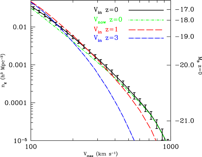
Figure 2.— The left-hand vertical axis shows the cumulative number density of galaxies in our simulation catalog as a function of velocity using $V_{now}$ at $z=0$ (dot-dash, current $V_{\rm max}$) and $V_{in}$ at $z=0$ (solid, the value of $V_{\rm max}$ when the halo was accreted) to identify subhalos as galaxies. The right-hand axis maps the $z=0$ B-band absolute magnitude of galaxies from the SSRS2 luminosity function to the appropriate galaxy number density shown on the left-hand vertical axis. Using the right-hand scale, the solid and dot-dashed lines demonstrate our adopted $z=0$ relationship between $V_{\rm in}$ or $V_{\rm now}$ and galaxy luminosity. The remaining two lines show the $V_{in}$ sample at $z=1$ and $z=3$. A comparison with Figure 1 reveals dramatic differences between the evolution of distinct host halo number densities and the galaxy (subhalo) number densities shown here. The errorbars shown were generated by summing in quadrature the jackknife error and the realization to realization scatter.

2.2. Substructure Model

In order to determine the substructure properties in each host dark matter halo, we model halo mass accretion histories and track their substructure content using an analytic technique that incorporates simplifying approximations and empirical relations determined via numerical simulation. We provide a brief overview of the technique. The model is described in detail in Zentner et al. (2005, hereafter Z05), and is an updated and improved version of the model presented in Zentner & Bullock (2003). This model shares many elements with similar models of Taylor & Babul (2004), Peñarrubia & Benson (2005), and van den Bosch et al. (2005).

In hierarchical CDM-like models, halos accumulate their masses through a series of mergers with smaller objects. Thus the first step of any analytic calculation is to build an approximate account of this merger hierarchy. For each host halo of mass $M$ at redshift $z$ in our numerical simulation volume, we randomly generate a mass accretion history using the extended Press-Schechter formalism (Bond et al., 1991; Lacey & Cole, 1993) with the particular implementation of Somerville & Kolatt (1999). The merger tree consists of a list of all of the distinct halo mergers that have occurred during the process of accumulating the mass of the final host object at the redshift of observation. Every time there is a merger, the smaller object becomes a subhalo of the larger object.

We then track the evolution of subhalos as they evolve in the main system in the following way. At each merger event, we assign an initial orbital energy and angular momentum to the infalling object according to the probability distributions culled from cosmological $N$-body simulations by Z05. We then integrate the orbit of the subhalo in the potential of the main halo from the time of accretion to the epoch of observation. We model tidal mass loss with a modified tidal approximation and dynamical friction using a modified form of the Chandrasekhar formula (Chandrasekhar, 1943) suggested by Hashimoto et al. (2003). For simplicity, we model the density profiles of halos using the Navarro et al. (1997, NFW) profile with concentrations set by their accretion histories according to the algorithm of Wechsler et al. (2002). As subhalos orbit within their hosts, they lose mass and their maximum circular velocities decrease as the profiles are heated by tidal interactions. A practical addition to this evolution algorithm is a criterion for removing subhalos from catalogs once their bound masses become so small as to render them very unlikely to host a luminous galaxy. This measure prevents using most of the computing time to evolve very small subhalos on very tightly bound orbits with very small timesteps. For the purposes of the present work, we track all subhalos until their maximum circular velocities drop below $V_{\rm max}=80$ km s^-1, at which point they are no longer considered and are removed from the subhalo catalogs. We refer the interested reader to § 3 of Z05 for the full details of this model.

The computational demands of this analytic model are such that we can repeat this process several times for each host halo in the simulation volume in order to determine the effect of the variation in subhalo populations among halos of fixed mass on our close pair results. For example, one source of noise is due to subhalo orbits: subhalos at pericenter are likely to be counted as close pairs, whereas subhalos at apocenter are less likely to be counted as close pairs. In order to make this assessment, we repeat this procedure for computing subhalo populations for each host halo in the computational volume thereby creating distinct subhalo catalogs with identical large-scale structure set by the large-scale structure of the simulation. We refer to each of these distinct subhalo catalogs as a “realization” of the model, a term which derives from the inherent stochasticity of the model. Additionally we may perform rotations of the simulation volume. These rotations provide us with different lines of sight through the substructure of the simulation. Since the perpendicular separation along the line of sight of the subhalos is extremely important to the close pair statistics, along with the velocity differences along these lines of sight, these rotations provide us with additional effective “realizations”. Three rotations are performed on each simulation box, providing us with more effective “realizations”.

This substructure model has proven remarkably successful at reproducing subhalo count statistics, radial distributions, and two-point clustering statistics measured in full, high-resolution $N$-body simulations in regimes where the two techniques are commensurable. The results of the model agree with full numerical treatments over more than $3$ orders of magnitude in host halo mass and as a function of redshift (Z05). This success motivates its use to overcome some of the difficulties associated with using a purely numerical treatment. Specifically, unlike N-body simulations, this method suffers from no inherent resolution limits and makes the process of selecting subhalo populations based on specific features of their merger histories or detailed orbital evolution clean and easy. Note that any correlation between formation history or the HOD and the larger scale environment will not be included in catalogs created with this hybrid method, but this is not expected to be important for most of the mass range we consider here (Wechsler et al., 2006).

We explore two simple yet reasonable toy models for associating galaxies with dark matter subhalos. In order to quantify the size of subhalos, we use the subhalo maximum circular velocity, $V_{\rm max}\equiv max[\sqrt{GM(<r)/r}]$. This choice is motivated by several considerations. As long as only systems that are well above any resolution limits are considered, this quantity is measured more robustly in simulation data and is not subject to the same ambiguity as particular mass definitions because $V_{\rm max}$ is typically achieved well within the tidal radius of a subhalo. These facts make our enumerations by $V_{\rm max}$ easier to compare to the work of other researchers using different subhalo identification algorithms. In the next section we describe our mapping of galaxies onto subhalos, and explore models for mapping galaxies onto subhalos that use the maximum circular velocities defined at two different epochs.

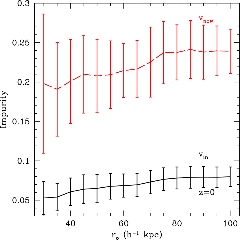
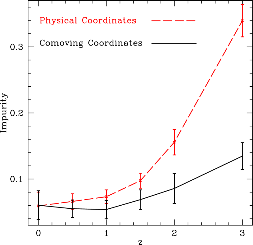
Figure 3.— Pair count impurity in our simulated galaxy catalogs with a fixed comoving number density $n_{g}=0.01h^{3}$ Mpc^-3. Impurity is defined to be the fraction of pair-identified galaxies that do not sit within the same host dark matter halo. The error bars represent variations in the impurity due to cosmic variance as well as variation in the subhalo populations. The uncertainties were calculated using the realization to realization scatter and the jackknife errors. Left: The $z=0$ impurity as a function of outer projected radius used for the pair criteria ($r_{o}$ in the text). Here we have fixed the inner radius for pair identification at $r_{i}=10~{}h^{-1}{\rm kpc}$ and demanded line-of-sight velocity separations to be within $\Delta v=\pm 500$km s^-1. The solid line represents the $V_{in}$ sample while the dashed line uses $V_{now}$. Right: The impurity as a function of redshift within a fixed physical separation of $r_{o}=50$ h^-1 kpc, using $V_{in}$. The red dashed line is the impurity in the pair fraction for a system in physical coordinates. The black solid line is the impurity in the comoving coordinates. Note that in most cases $\lower 2.58334pt\vbox{\hbox{$\buildrel\textstyle>\over{\sim}\ $}}90\%$ of galaxies identified as close pairs by these observationally-motivated criteria inhabit the same host dark matter halo for $z\leq 1.5$. In the physical coordinates we see a sharp rise in the impurity beyond this redshift.

2.3. Assigning Galaxies to Halos and Subhalos

After computing the properties of halos and subhalos in a $\Lambda$CDM cosmology, the next step is to map galaxies onto these objects. In our comparisons with observational data, we normalize our model galaxy catalogs to an observed population by matching their mean number densities to those of halos and subhalos. In each case, we assume that there is a monotonic relationship between halo circular velocity, $V_{\rm max}$, and galaxy luminosity in the relevant band of interest. The number density of galaxies as a function of halo (subhalo) $V_{\rm max}$ is shown in Figure 2. For our $z=0$ comparisons we adopt the SSRS2 B-band luminosity function in order to match the samples appropriately. The implied mapping between $M_{\rm B}$ and $V_{\rm max}$ for the SSRS2 luminosity function is demonstrated in the right y-axis of Figure 2. For the Lin et al. (2004) DEEP2 comparison at $z\simeq 0.5-1.1$ we match our $V_{\rm max}$ functions with the measured luminosity function in the $R_{\rm AB}$ band.

Although a monotonic relationship between $V_{\rm max}$ and luminosity is a simplifying assumption, it serves as a useful, physical model for our comparisons, and is motivated in part by the well-known Tully-Fisher relation which shows that the observed speed of a spiral galaxy correlates with its luminosity in all bands (Tully & Fisher, 1977). Scatter in this relationship could (of course) be included in our model, but we have chosen to neglect this for the sake of simplicity. Moreover, a number of studies have demonstrated that threshold samples selected in this way exhibit excellent agreement with many of the clustering statistics of observed galaxy samples (e.g., Klypin et al., 1999; Kravtsov et al., 2004a; Tasitsiomi et al., 2004; Azzaro et al., 2005; Conroy et al., 2006, ; Marin, Wechsler & Nichol, in preparation). The decision to normalize our catalogs based on the number densities of halos and subhalos above thresholds in maximum circular velocities circumvents the need to model star formation directly in our simulations and allows us to focus on well-understood physical parameters. As we demonstrate below, close pair fractions vary strongly with galaxy number density at fixed redshift.

For subhalos, a monotonic relationship between current maximum circular velocity and galaxy luminosity is less well-motivated than it is for host halos (or halos in the “field”). When a halo merges into a larger host halo and becomes a subhalo, it loses mass as a result of tidal interactions and its maximum circular velocity decreases. The degree to which luminosity is lost or surface brightness declines is considerably more uncertain (see, e.g. Bullock & Johnston, 2005, and Bullock & Johnston, in preparation), but is probably less than the decrease in mass (e.g. Nagai & Kravtsov, 2005) Using maximum circular velocities rather than total bound masses partly accounts for this mismatch between mass and luminosity because maximum circular velocity scales only very slowly with bound mass, $V_{\rm max}\propto M^{\gamma}$, with $\gamma\sim 0.25$ (Kravtsov et al., 2004b; Kazantzidis et al., 2004). In addition, environmental effects add a further complication as they may influence the luminosity or star formation rate of a galaxy in such a way that it is driven off of any $V_{\rm max}$-luminosity relationship that may exist in the field.

We deal with this uncertainty by adopting two simple models for associating subhalos with galaxies: first, the maximum circular velocity that the subhalo had when it was first accreted into the host halo, $V_{\rm in}$, and second, the maximum circular velocity that the subhalo has at the current epoch, $V_{\rm now}$. The choice of $V_{\rm in}$ mimics a case where a galaxy is much more resistant to reductions in luminosity than the dark matter subhalo is to mass loss. The choice of $V_{\rm now}$ represents a case where a galaxy drops out of a luminosity threshold sample (or, perhaps more realistically, a surface-brightness threshold sample) in direct proportion to the decline in the maximum circular velocity of the subhalo.

As we stated above, subhalo $V_{\rm max}$ declines much more slowly than total bound mass during episodes of mass loss, so both methods assume that the luminosity of the galaxy is resistant to large changes resulting from the early stages of interaction, which is supported by observations of pairs at low redshifts (Barton et al., 2001; Barton Gillespie et al., 2003). In the case of $V_{\rm in}$, the luminosity is set in the field and does not change after merging into the host system, while in the case of $V_{\rm now}$ the luminosity declines slowly as a result of interactions with the host system.

The $V_{\rm in}$ choice is likely the most natural one, and has been shown to provide an excellent match to clustering statistics over a range of redshifts for scales larger than 100 $h^{-1}{\rm kpc}$ (Conroy et al., 2006). However, the $V_{\rm now}$ model provides acceptable clustering statistics at large separations (Kravtsov et al., 2004a), and provides a very useful reference point for exploring the uncertainty in theoretical predictions of close pair fractions and for highlighting the type of physical processes that close pairs can and cannot probe.

We emphasize that the evolution of the host halo merger rate is not an appropriate comparison for the evolution of close pair counts, which probe the galaxy or subhalo merger rate. The models we examine represent two different choices for how galaxies populate their hosts. The fact that the $V_{\rm in}$ and $V_{\rm now}$ models both have the same host halo merger rates, but different halo occupation counts that result in very different predictions for small-scale clustering, highlights the fact that close pairs are not directly connected to halo merger rates except in the context of a specific model for how galaxies populate these halos.

Figure 2 shows the cumulative number density of “galaxies” identified in our simulations, $n_{g}$, as a function of their maximum circular velocities. The solid line shows $z=0$ galaxies using $V_{\rm in}$ as an identifier. The dash-dot line shows the same using $V_{\rm now}$. The $V_{\rm now}$ choice lies below $V_{\rm in}$ because galaxies more readily fall out of the observational sample in this case due to the mass lost by the subhalo after accretion. Note that host halos always have $V_{\rm now}=V_{\rm in}$. The fact that the $V_{\rm now}$ and $V_{\rm in}$ number density lines differ by only $\sim 30\%$ reflects the fact that most galaxies are field galaxies and this choice affects only the satellites of group and cluster systems. The right y-axis for the solid and dash-dot lines in Figure 2 illustrates how this choice affects our mappings between velocity and galaxy luminosity at $z=0$. The dashed and long-dash-dot lines show $n_{g}$ for the $V_{\rm in}$ choice at $z=1$ and $z=3$. The luminosity function used is the combined SSRS2 luminosity function (Marzke et al., 1998). Compared with Figure 1 we see that the galaxy velocity function evolves much more weakly with redshift than does the host halo mass function.

2.4. Defining Close Galaxy Pairs and Diagnosing the Effect of Interlopers

Various definitions have been used for identifying close pairs of galaxies (e.g., Kennicutt & Keel, 1984; Zepf & Koo, 1989; Burkey et al., 1994; Carlberg et al., 1994; Woods et al., 1995; Yee & Ellingson, 1995; Barton et al., 2000; Patton et al., 2000; Carlberg et al., 2000; Bundy et al., 2004; Le Fèvre et al., 2000; Patton et al., 2002, 1997; Neuschaefer et al., 1997). In this work we follow the definition used in Patton et al. (2002) and Lin et al. (2004), and use the average number of companions per galaxy to enumerate close galaxy pairs:

$$N_{c}\equiv\frac{2n_{\rm p}}{n_{g}}.$$ (1)

In Eq. (1), $n_{g}$ is the number density of galaxies in the sample and $n_{\rm p}$ is the number density of individual pairs.

We define pairs as galaxies that fall within a well-defined line-of-site velocity separation $|\Delta v|$ and that have a projected, center-to-center separation on the sky, $r_{\rm p}$, that lie between an inner and outer value $r_{i}<r_{\rm p}<r_{o}$. The inner radius is chosen to prevent morphological confusion. The outer radius may be adjusted to reduce contamination of the sample by interlopers. We use fiducial values of $r_{i}=10h^{-1}{\rm kpc}$ and $r_{o}=50h^{-1}{\rm kpc}$ in physical units and we adopt a fiducial relative line-of-sight velocity difference of $|\Delta v|=500$ km s^-1, following Patton et al. (2002) and Lin et al. (2004). In what follows, we refer to the chosen close-pair volume as a “cylinder”. We emphasize that in our standard measure we adopt physical radii and a constant $\Delta v$ cut to define our cylinder at all redshifts (“physical cylinder”), but we also explore a case where the radii and line-of-sight depth (defined by $\Delta v$) are scaled with the expansion of the universe (“comoving cylinder”).

Our model catalogs provide a useful tool for studying the degree of contamination by interlopers in this commonly-adopted measure. If we define interlopers as projected galaxy pairs that do not lie within the same host halo, we can define a measure of close pair count impurity as

$${\rm Impurity}\equiv\frac{n_{f}}{n_{p}},$$ (2)

where $n_{f}$ is the number density of interloping, or false pairs in the sample and $n_{p}$ is the total number density of observed pairs.

The left panel of Figure 3 shows how the impurity varies as a function of the choice of outer pair radius $r_{o}$ for both $V_{in}$ (solid) and $V_{now}$ (dashed) samples at $z=0$. For each choice, we fix $r_{i}=10h^{-1}{\rm kpc}$ and define the galaxy population using a galaxy number density $n_{g}=0.01h^{3}$ Mpc^-3. The $V_{\rm now}$ case has a higher overall impurity ($\sim 20\%$ compared to $\sim 5\%$), reflecting the fact that the amplitude of $N_{c}$ is generally lower for $V_{\rm now}$ (see §3 ) and is therefore more affected by chance projections. Both the $V_{\rm in}$ and $V_{\rm now}$ samples show only a mild increase ($\sim 3\%$) in the interloper fraction as the outer cylinder radius is varied from $r_{o}=30$ $h^{-1}{\rm kpc}$ to $100$ $h^{-1}{\rm kpc}$.

The right panel of Figure 3 shows the impurity as function of redshift for the $V_{\rm in}$-selected sample. The dashed line corresponds to a physical cylinder and the solid line corresponds to a comoving cylinder at the same fixed comoving number density $n_{g}=0.01h^{3}$ Mpc^-3. Both lines have $r_{o}=50h^{-1}{\rm kpc}$. The impurity in the comoving cylinder remains relatively small with $z$, while for the physical cylinder, the fraction of interlopers remains small until $z\sim 2$, after which it rises sharply. This reflects the fact that halo virial radii scale as $\sim(1+z)^{-1}$ and become a smaller fraction of a fixed physical $r_{o}$ at high redshift. While one might interpret this result as favoring the use of a comoving cylinder for pair identification, there are practical difficulties in resolving pairs at small comoving separations at high redshift. For example, while physical separations between $r_{p}=10-50$ $h^{-1}{\rm kpc}$ correspond to resolvable angular separations at $z=2$, $\theta_{p}\simeq 1.7-8.5$ arc seconds, the corresponding comoving distances would be much more difficult to resolve, $\theta_{p}\simeq 0.57-2.8$ arc seconds. Ground based surveys require separations $>2$ arc seconds (Bell et al., 2006). The main conclusion to draw from this figure is that for most practical pair measures, interlopers will be of increasing importance at high redshift.

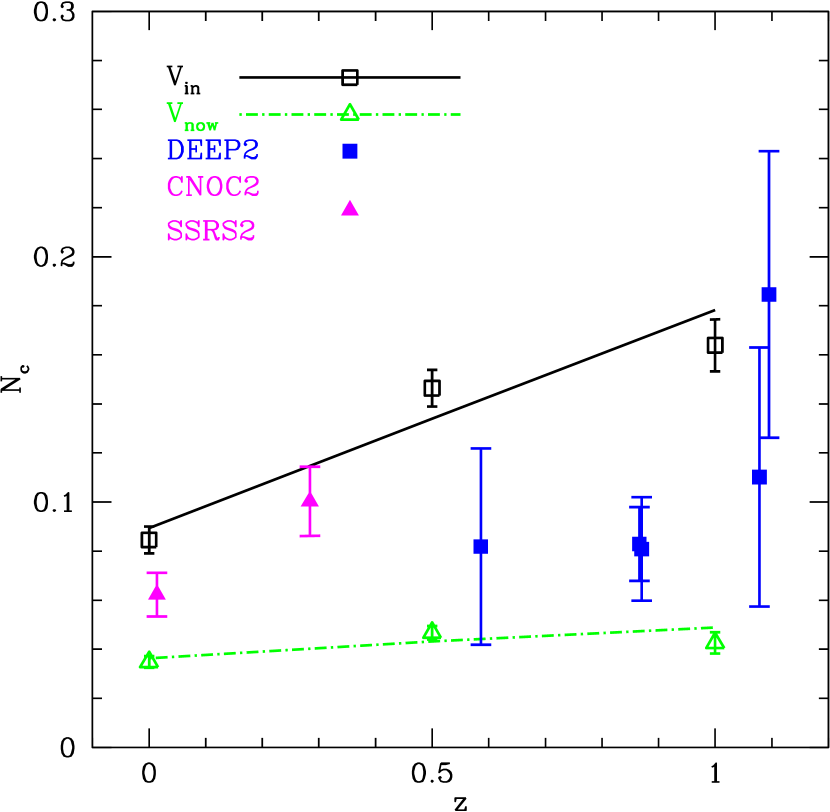
Figure 4.— Evolution in the companion fraction. Solid squares are data points from the DEEP2 Survey taken from fields 1 and 4, (Lin et al., 2004). Close companions are defined as having physical separations between $r_{p}=10-50$ $h^{-1}{\rm kpc}$ with a line of sight velocity difference of $<500$ km s^-1. Solid triangles are data from CNOC2 and SSRS2, (Patton et al., 2002). The empty points with best-fit lines are taken from our simulations. At each redshift we select model galaxies by approximately matching the number densities of galaxies used in the DEEP2, SSRS2, and CNOC2 points to the nearest simulation redshift. Empty triangles use $V_{\rm now}$ velocity function to match number densities while empty squares use $V_{\rm in}$. Lines show the best-fit to $N_{c}\propto(1+z)^{m}$ with $m=0.42\pm 0.17$ ($V_{\rm now}$) and $m=0.99\pm 0.14$ ($V_{\rm in}$). In both cases the predicted evolution is quite weak and broadly consistent with the data.

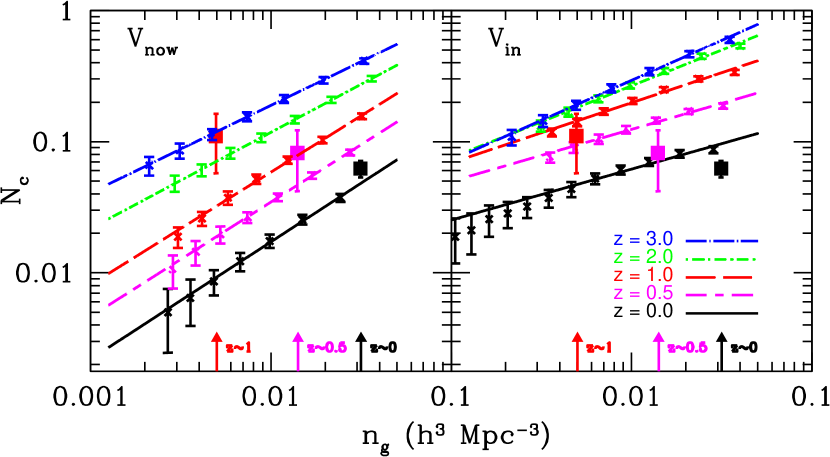
Figure 5.— Close companion fraction as a function of number density and redshift for a fixed physical separation between $r_{i}=10h^{-1}{\rm kpc}$ and $r_{o}=50h^{-1}{\rm kpc}$ in projection and a line-of-sight velocity difference $|\Delta v|\leq 500$ km s^-1. Small points with linear fits show the the average number of close companions $N_{c}$, as a function of galaxy number density $n_{g}$, for our model with galaxy selection based on $V_{\rm now}$ (left panel) and $V_{\rm in}$ (right panel). The five lines show power-law fits of the companion fraction at $z=0$, $0.5$, $1$, $2$, and $3$ (from bottom to top) to the form $N_{c}\propto n_{g}^{a}$. The best-fit slopes vary from $a=0.89\pm 0.09$ at $z=0$ to $a=0.67\pm 0.07$ at $z=3$ for galaxy samples selected on $V_{\rm now}$ and from $a=0.39\pm 0.07$ at $z=0$ to $a=0.61\pm 0.04$ at $z=3$ for samples selected on thresholds in $V_{\rm in}$. Large, solid points represent observational data points shown in Figure 4. These points are taken from the three nearest redshift bins to $z\simeq 0$, $0.5$, and $1.0$, and plotted at the number densities of the data samples. Arrows along the bottom edge of the figure indicate the redshift corresponding to each of these data points. The decreasing number densities with increasing redshift in the observational samples results in a nearly constant value of the companion fraction with redshift. The data seem marginally to favor the $V_{\rm in}$ model over $V_{\rm now}$.

3. Results

3.1. Evolution in Companion Counts

We first present results on the overall evolution of close companion counts with redshift. Figure 4 shows our model results for the companion fraction of galaxies, $N_{c}$, as a function of redshift for our $V_{\rm in}$ selection (open squares, with line fits) and our $V_{\rm now}$ selection criterion (open triangles, with line fits) compared with some recent observational measurements. Solid squares are data from the Lin et al. (2004) DEEP2 analysis (fields 1 and 4). Solid triangles at lower redshift reflect data from the Second Canadian Network for Observational Cosmology (CNOC2) survey and data from SSRS2 (Patton et al., 2002).

As was found in the observational sample of Lin et al. (2004), the companion count exhibits very weak evolution when plotted in this manner. It is also evident that both the $V_{\rm in}$ and $V_{\rm now}$ models show similarly weak evolution and seem to be broadly consistent with the observational data. The formal fit by Lin et al. (2004) from this data gives close pair evolution as $N_{c}\propto(1+z)^{m}$, with $m=0.51\pm 0.28$. A similar fit to our model results, from $z=0$ to $z=1$, shown in Figure 4 yields $m=0.42\pm 0.17$ for selection on $V_{\rm now}$, and $m=0.99\pm 0.14$ for sample selection based on $V_{\rm in}$. Note that the $V_{\rm in}$ points are systematically higher than the $V_{\rm now}$ points. This reflects the fact that galaxies are more easily driven out of an observable sample by tidal mass loss in the $V_{\rm now}$-selected sample (see § 4 for a more detailed discussion).

While Figure 4 seems relatively simple upon first examination, the broad agreement between simulation results and the data is attained because we have been careful to normalize the data and theory in a consistent manner. Each of the DEEP2 points correspond to different underlying galaxy number densities. This was done in order to account for gross luminosity evolution with redshift, $z$, assuming a simple model where $M(z)=M(0)-z$. In order to make a fair comparison with their results, we have forced the mean number density of the model galaxies to match the corresponding observed number density of galaxies by varying the maximum circular velocity threshold (using either $V_{\rm in}$ or $V_{\rm now}$). This technique corresponds to re-normalizing the relationship between $V_{\rm in}$ (or $V_{\rm now}$) and galaxy luminosity at each redshift.

Using the correct number density for comparison at each redshift is of critical importance. In Figure 5, we plot the companion fraction as a function of comoving galaxy number density $n_{g}$ in our model catalogs (small points with line fits) using $V_{\rm now}$ (left panel) and $V_{\rm in}$ (right panel) for five redshift steps between $z=0.0$ and $z=3.0$. For both models, at fixed $z$, the companion fraction increases with the overall galaxy number density, while at fixed comoving number density the companion fraction increases with redshift. The number densities and close pair counts for selected data points in Figure 4 are represented as large, solid squares in Figure 5. An approximate redshift for each of the data points is indicated by an arrow along the bottom of the plot. Comparing the lines with the solid squares in Figure 5 illustrates that the $N_{c}(z)$ points in Figure 4 show little evidence for evolution simply because they correspond to lower number densities at higher redshifts. An analytic explanation for how $N_{c}$ scales with number density is given in the Appendix, where we also present $z=0$ correlation functions for the $V_{\rm max}$ models at different values of $n_{g}$.

3.2. $z=0$ Companion Counts

The trend with $N_{c}$ and $n_{g}$ seen in the simulations leads us to look for such a trend in some observational samples. To compare with $z=0$ galaxies, we must balance the need for a large comparison redshift survey that fairly samples large-scale structure with the requirement for completeness with close galaxy pairs. Our approach is to use small but nearly complete redshift surveys and to examine the effects of cosmic variance a posteriori.

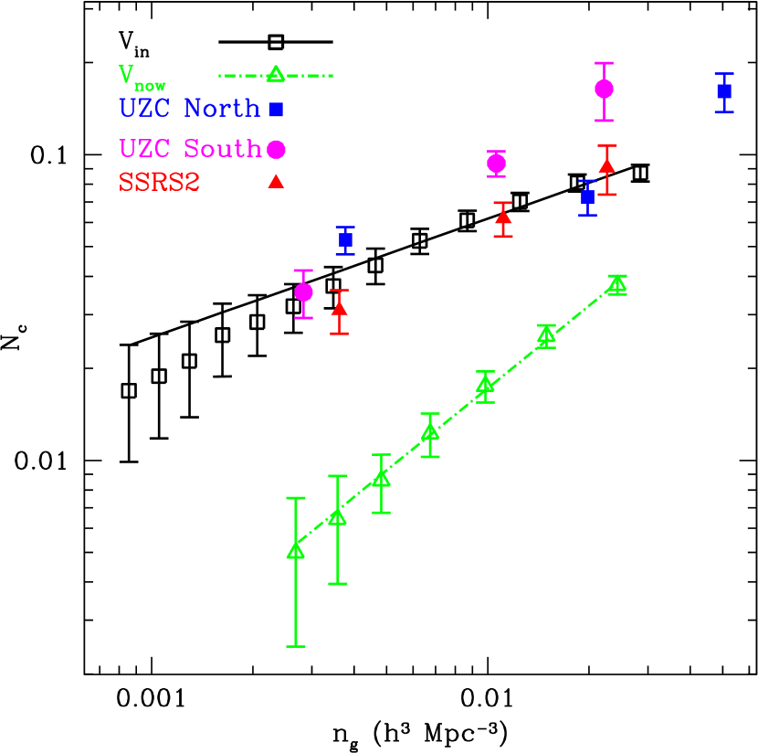
Figure 6.— The variation of $N_{c}$ at $z=0$ based on the number density, $n_{g}$, of galaxies in the sample. We vary galaxy number density by making different threshold cuts in $V_{in}$ and $V_{now}$. Close companions are defined as having physical separations between $r_{p}=10-50$ $h^{-1}{\rm kpc}$ with a line of sight velocity difference of $<500$ km s^-1. Notice that pair counts based on galaxies selected according to $V_{in}$ are comparable to data from both the UZC and SSRS2 redshift surveys. In addition, note the radically different slope for the $V_{now}$ line as well as its under-prediction of $N_{c}$. The points along the $V_{in}$ line represent the average over three rotations of the four realizations at cuts ranging from $V_{in}=110-350$ in steps of 20 km s^-1. For $V_{now}$ the points range from $V_{\rm now}=110-230$ in steps of 20 km s^-1. The observational data points clearly favor the $V_{\rm in}$ model over the $V_{\rm now}$ model.

In Figure 6 we show the close companion fraction $N_{c}$, derived from galaxies taken from the UZC (solid squares for the North field and solid circles for the South) and the SSRS2 and CNOC2 (solid triangles) redshift surveys as a function of galaxy number density using the measured luminosity functions for the UZC-CfA2 North, UZC-CfA2 South, and SSRS2 surveys (Marzke et al., 1994; Falco et al., 1999; Fasano, 1984; Patton et al., 2000). The CfA2 North field originally covered a range of declination from $8.5^{\circ}\leq\delta\leq 44.5^{\circ}$. For it’s Northern field CfA2 has a right ascension range of $8^{h}\leq\alpha\leq 17^{h}$, Geller & Huchra (1989); Huchra et al. (1990, 1995). The original CfA2 South field covers a range of declination from $-2.5^{\circ}\leq\delta\leq 48^{\circ}$. The CfA2 survey’s southern field has a right ascension range of $20^{h}\leq\alpha\leq 4^{h}$, Giovanelli & Haynes (1985); Giovanelli et al. (1986); Haynes et al. (1988); Giovanelli & Haynes (1989); Wegner et al. (1993); Giovanelli & Haynes (1993). The CfA2 North field has $6500$ galaxies while the South field has $4283$ galaxies originally cataloged. These are volume-limited samples from $2300\leq cz\leq{\rm H_{0}}10^{G({\rm M_{B,lim}})}$ km s^-1. Here the exponent $G({\rm M_{B,lim}})=(15.5-{\rm M_{B,lim}}-25)/5$ is a function of a variable limiting magnitude and $M_{B}=15.5$ is the limiting apparent magnitude of the surveys. We derive number densities for each point by integrating the luminosity function from ${\rm M_{B,lim}=-18}$,$-19$, and $-20$, respectively to a minimum magnitude of $M_{B}=-30$. Note that within the same survey the data points are not independent. Differences among the surveys arise, in part, because of differences in large scale structure, see §3.3.

The results of our model pair counts are also shown in Figure 6 for both selection on $V_{\rm in}$ (open squares) and selection on $V_{\rm now}$ (open triangles). The data clearly favor the higher pair counts that follow from selecting galaxies based on the initial maximum circular velocities of their subhalos when they entered their hosts, $V_{\rm in}$. The $V_{\rm now}$ selection under-predicts the data by a factor of $\sim 3-5$, depending on the number density. We emphasize that both initial circular velocity and final circular velocity selections are made from the same underlying population of host dark matter halos, which thus have identical merger histories and instantaneous merger rates. The differences in pair counts reflect only differences in the evolution of satellite galaxies within their host dark matter halos.

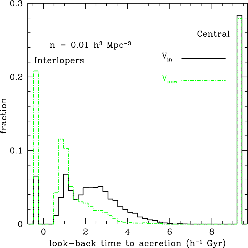
Figure 7.— Fraction of unique pair-identified galaxies with a given lookback accretion time. We include each galaxy identified as part of a unique $z=0$ pair and use $\ng=0.01$ h³ Mpc^-3 with $Vin$ (solid) and $V_{\rm now}$ (dashed). If a pair of galaxies sits in different host halos, then each galaxy is assigned an (unphysical) negative accretion time and placed in the far left bin (interlopers). If a pair of galaxies sits in the same host halo, then each galaxy is assigned the time it was accreted into the host. If one of the same-halo paired galaxies happens to be a central object, we set the lookback accretion time to be the age of the universe (far right bin).

While the host dark matter halo merger rates are identical between the $V_{\rm in}$ and $V_{\rm now}$ models, the accretion times of the galaxy-identified subhalos in the two cases are significantly different. Figure 7 shows the distribution of lookback accretion times for each object identified in a unique galaxy pair at $z=0$ for $n_{g}=0.01h^{-3}\rm Mpc^{3}$ using $V_{\rm in}$ (solid) and $V_{\rm now}$ (dashed). In this figure every unique galaxy pair is assigned two accretion times, one for each galaxy involved in the pair. For example, if there are $N$ close companions then we include $N(N-1)$ accretion times for those galaxies. If a pair of galaxies is contained in the same host halo, we assign each galaxy a time based on its time of accretion into the host halo. If one of the same-halo objects is a central galaxy, we let its “accretion time” be the age of the universe (far right bin). If the two galaxies identified as a unique pair are part of different halos (interlopers) we assign each galaxy an unphysical, negative accretion time (the far left bin). 

The far right bin in Figure 7 shows that $\sim 28\%$ of galaxies in close companions correspond to central objects. However, note that if we were enumerating pairs rather then the galaxies in the pairs, most pairs on these scales, in our case $\sim 56\%$, would consist of a satellite and a central object, as one might expect from the familiar “one halo term” in the halo model.   Similarly, $\sim 5\%$ ($\sim 20$) of paired galaxies are “interlopers” sitting in different host halos (far left bin) for the $V_{\rm in}$ ($V_{\rm now}$) choice. As seen in the central histogram, most unique pair-identified galaxies are subhalos. The $V_{\rm now}$-chosen satellite pairs tend to be accreted fairly recently, within the last $\sim 0.5-2$ $h^{-1}$ Gyr. On the other hand, the $V_{\rm in}$ galaxies can survive longer within the host potential without dropping out of the observable sample, and have a fairly broad range of accretion times ($\sim 1-4$ $h^{-1}$  Gyr). More generally, we see that the inferred accretion time distribution for observed galaxy pairs will depend sensitively on galaxy formation assumptions.

3.3. Cosmic Variance

Cosmic variance is a major concern for the result presented in Figure 6. The UZC and SSRS2 surveys both contain structures that are comparable in size to the surveys as a whole, and are therefore not “fair” samples of the large-scale structure of the universe. For example, the data clearly reflect the fact that the SSRS2 survey is underdense relative to UZC. Here, we investigate whether the high observed pair fractions could simply reflect an overdensity on a scale comparable to that of the surveys.

To examine the uncertainty in pair counts due to cosmic variance in more detail we performed mock observations of subsets of our full simulation volume to determine the variation in the pair counts in volumes comparable in size to the survey volumes. Figure 8 shows the variation in $N_{c}$ over eight cubic regions of the simulation for each realization, each $60h^{-1}{\rm Mpc}$ on a side for a volume of $2.16\times 10^{5}h^{-3}$ Mpc³. This sub-volume is within 12% of the the volume-limited UZC survey to M${}_{\rm B,lim}=-19$. It is roughly half of the volume for the M${}_{\rm B,lim}=-20$ points for UZC-CfA2 North and UZC-CfA2 South; and more than twice the volume for the M${}_{\rm B,lim}=-19$ SSRS2 point. For each octant, we plot twelve values of $N_{c}$: each of the three projections through the box along with four statistical subhalo realizations for each projection. The four symbol types correspond to each of the four realizations and we have introduced a slight horizontal shift to reflect the three sets of rotational projections. We select model galaxies by fixing the number density to $n_{g}=0.01h^{3}$ Mpc^-3 within the full box. This corresponds to a limit of $V_{\rm in}\gtrsim 162$ km s^-1. The reason for this approach is that it mimics what is done in the observational sample, and uses the same effective luminosity function for the whole volume of the box. If we instead choose the same number density within each sub-volume of the box, the overall octant-to-octant scatter is reduced by a factor of $\sim 2$. The solid line represents the mean over all $96$ points, while the dot-dashed line shows the RMS variation: $N_{c}=0.063\pm 0.011$. Using only one projection yields a nearly identical result. Error bars on each point are Poisson errors on the number of pairs and reflect the expected variation in pair counts in the absence of cosmic variance. Notice that the scatter is somewhat larger than what would be expected from shot noise.

As we see from Figure 8, at maximum the octant-to-octant (large-scale structure) variation is $\sim 50\%$. This is much smaller than the $\sim 300\%$ variation required to reconcile the $V_{\rm now}$ model with the data. We also note that the scatter within the local surveys is much smaller than the variation required to reconcile the $V_{\rm now}$ model with the observational data sets. Nonetheless, repeating this experiment with a larger survey with better completeness will be required to verify this agreement.

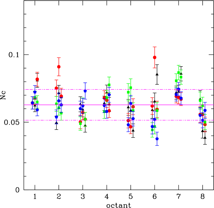
Figure 8.— Testing the importance of cosmic variance in the observational data sets. We show $N_{c}$ measured in each octant (1-8 on the horizontal axis) of the simulation volume for each of the four Monte-Carlo subhalo realizations (four symbol types at each octant number) and for three rotations of each simulation box, the points offset from each octant. Error bars on subhalo realizations reflect Poisson errors on the number of pairs. Here we select model galaxies using a fixed $V_{\rm in}\simeq 162$ km s^-1, which corresponds to a number density within the full box of $n_{g}=0.01h^{3}$ Mpc^-3. The mean, over all of the companions fractions, is given by the solid line while the dot-dashed lines show the RMS variation, $0.063\pm 0.011$. This mean value does not significantly differ from those produced using only one of the possible lines of sight.

3.4. General Predictions

Figure 5 illustrated our expectation that the average companion number $N_{c}$, within a fixed physical cylinder volume increases with redshift at fixed mean co-moving number density. However, this increase does not reflect the increased merger activity associated with hierarchical structure formation. In fact, the predicted evolution is driven primarily by the choice of a fixed physical cylinder to define pairs rather than a selection volume that is fixed in comoving units. Figure 9 shows the identical statistic computed from our model galaxy populations using the selection on $V_{\rm in}$ at $z=0,1$, and $3$, but this time using the comoving cylinder (with volume $\propto(1+z)^{3}$). The virialized radius of host halos at fixed mass decreases with redshift roughly as $R_{\rm vir}\propto(1+z)$. With these new coordinates we continue to probe the same “fraction” of each halo (of fixed mass) over the entire redshift range. First, notice that in comoving units the variation in pair counts with redshift is much more mild than it is in physical units. The counts in Figure 9 span at most a factor of two while the counts in Figure 5 span more than an order of magnitude over an identical redshift range. Second, after normalizing out the effect of the cosmological expansion, the pair count per galaxy actually decreases with redshift rather than increasing as shown in Figure 5.

The primary reason why the companion fraction does not evolve strongly with redshift is that the number density of host halos massive enough to host more than one bright galaxy decreases at high redshift. This is shown explicitly in Figure 10, where we plot the distribution of host halo masses for galaxies (solid lines with error bars, left axis) at $z=0$ and $3$ using $V_{\rm in}$ to fix $n_{g}=0.01h^{3}{\rm Mpc}^{-3}$. The dashed line in each panel (right vertical axis) shows the distribution of host halo masses for pairs identified in the same sample of galaxies. At all redshifts, pairs are biased to sit in the most massive host halos. At high redshift massive halos become rare, and the pair fraction is reduced accordingly.

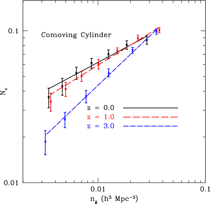
Figure 9.— The average companion count as a function of ($V_{\rm in}$-identified) comoving volume, $n_{g}$, using a cylinder with fixed comoving volume for companion identification. We see that once the expansion of the universe is accounted for the companion count per galaxy is predicted to decrease with redshift at fixed comoving number density (compare to Figure 5, which uses a fixed physical cylinder volume in defining $N_{c}$).

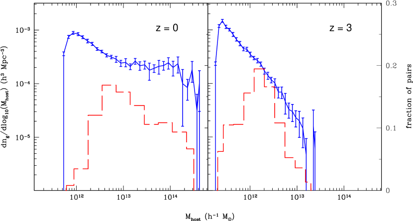
Figure 10.— The total galaxy number density distribution as a function of galaxy host halo mass (solid lines, left axis) compared to the distribution of host halo masses for identified galaxy pairs (dashed lines, right axis). In each case we use the $V_{\rm in}$ model with $n_{g}=0.01$ h³ Mpc^-3. Paired galaxies are biased to sit in larger halos than their “field” counterparts. At high redshifts, the larger host halos become increasingly rare, and this is reflected in distribution of host masses for paired galaxies.

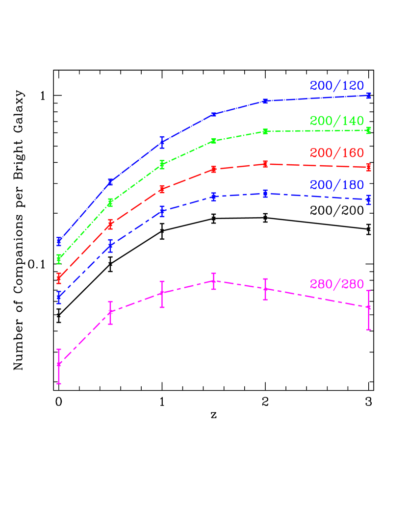
Figure 11.— The average number of close companions per bright galaxy as a function of redshift defined using our standard definition of close pair with a fixed physical separation. In all but the lowest line, “Bright” objects are defined as objects with a $V_{in}>200$ km s^-1. The pair fraction for “Bright-Bright” pairs is shown by the solid line (marked “200/200”) and even brighter “Bright-Bright” pairs (using $V_{\rm in}>280$ km s^-1) as the lowest long-short-dashed line (marked “280/280”). The other lines show the average “faint” companions per bright galaxy. We identify “Faint” objects using cut-offs of $V_{in}\geq X$ km s^-1 with $X=180,160,140,$ and 120. Not only is the faint companion fraction systematically higher than the bright companion fraction, it also evolves more strongly with redshift – a factor of $\sim 10$ out to $z\sim 2$ for the $200/120$ case compared to a factor of $\sim 3$ for the $200/200$ case. Note that the brightest “Bright-Bright” companion count shows a definite drop beyond $z\sim 1.5$.

Given that halos with multiple bright galaxies are expected to become increasingly rare at high redshift, faint companion counts may provide a more useful probe. Figure 11 shows the evolution in the average number of “Faint” companions per “Bright” galaxy as a function of redshift using our standard fixed physical separation criteria for defining close pairs. The top (dot-dashed) line shows the average number of “Faint” close companions with $V_{\rm in}>120$ km s^-1(${\rm M_{B}}\lesssim-17.3$ at $z=0$) around “Bright” galaxies with $V_{\rm in}>200$ km s^-1(${\rm M_{B}}\lesssim-18.9$ at $z=0$) as a function of $z$. The four lines below this restrict companions to be “brighter” galaxies with $V_{\rm in}=140$, $160$, $180$, and finally $200$ km s^-1. The last of these four (solid line) represents our standard “Bright-Bright” companion count, $N_{c}$. Finally, the lowest line shows the evolution in “Very Bright-Very Bright” companion counts using $V_{\rm in}=280$ km s^-1(marked “280/280”). As expected, the faint companion fraction is systematically higher than the bright companion fraction, but it also evolves more strongly with redshift. On average, almost every “Bright galaxy” (with $V_{\rm in}>200$ km s^-1) at $z>2$ is expected to host a “faint” companion (with $V_{\rm in}>120$ km s^-1). The “200/120” Bright-Faint companion count rises by almost a factor of $\sim 10$ between $z=0$ and $z=2$, while the increase is only a factor of $\sim 3$ for the $200/200$ case. Indeed the brightest “Bright-Bright” companion count (280/280) actually declines beyond $z\sim 1.5$. These trends reflect both the decline of massive halos at high redshift and the competition between accretion and disruption of subhalos, which favors accretion at high redshift.

4. Interpretations and the Halo Model

As demonstrated above, predicted (physical) close pair counts do not evolve rapidly with redshift, even at fixed global number density. This result is driven by a competition between increasing merger rates and decreasing massive halo counts: while the number of galaxy pairs per host halo increases with $z$ (as the merger rate increases), the number of halos massive enough to host a pair decreases with $z$. In this section we will work towards a more precise explanation and compare our two models for the connection between galaxy light and the subhalo properties $V_{\rm in}$ and $V_{\rm now}$, by investigating their Halo Occupation Distributions (HOD).

The HOD is the probability, $P(N|M)$, that $N$ galaxies meeting some specified selection criteria reside within the virial radius of a host dark matter halo of mass $M$. In what follows, we provide a brief introduction to the HOD as used in galaxy clustering predictions and use a “toy” HOD model to show that galaxy close companion counts provide an important constraint on the HOD and the distribution of galaxies within halos (see also Bullock et al., 2002). We then quantify our two subhalo models, $V_{\rm in}$ vs. $V_{\rm now}$, in terms of these inputs and present this as a general constraint on the kind of HODs required to match the current pair count data.

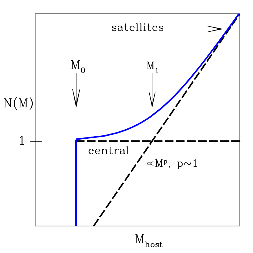
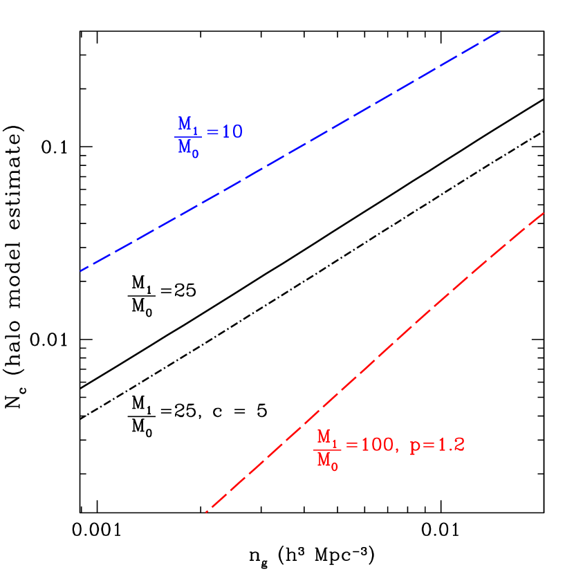
Figure 12.— Left: A cartoon representation of an input halo model $N(M)$, where the plateau at $N(M)=1$ represents central objects and the power-law piece, $\propto M^{p}$, represents satellite galaxies around the central galaxy. The ratio of $M_{0}$ to $M_{1}$ sets the importance of satellite galaxies compared to “field” galaxies – the larger the ratio, the more $n_{g}$ will depend on central, $N=1$, galaxies. Right: The pair fraction as estimated by a simple halo model calculation (see Equation 7 and associated discussion). Each line is labeled with its assumed ratio of $M_{0}/M_{1}$. As expected, models with a larger $M_{0}/M_{1}$ ratios have fewer companions per galaxy because field galaxies are emphasized. All lines assume a power-law index of $p=1.0$ except for the lowest dashed line with $p=1.2$. In this case, the relation with $n_{g}$ is steeper because satellite galaxies tend to be more plentiful in lower-mass host halos. The line labeled “$c=5$” has a more diffusely packed satellite distribution and as a result produces fewer close pairs with all other parameters held fixed.

4.1. Pair counts via the halo model

The halo model is a framework for calculating the clustering statistics of galaxies by assuming that all galaxies lie in dark matter halos (e.g. Seljak, 2000; Peacock & Smith, 2000; Scoccimarro et al., 2001). This approach relies on the fact that the clustering properties and number densities of host dark matter halos can be predicted accurately, and uses a parameterized HOD to make the connection between dark matter halos and galaxies.

Consider an HOD which consists of a “central” and “satellite” population of galaxies orbiting in the same dark matter halo (e.g. Kauffmann et al., 1993; Kravtsov et al., 2004a; Tinker et al., 2005; Cooray & Milosavljević, 2005). The total HOD is then described by two distributions $P(N_{c}|M)$ and $P(N_{s}|M)$ with individual mean values $N_{c}(M)=\int N_{c}P(N_{c}|M){\rm d}N_{c}$ and $N_{s}(M)=\int N_{s}P(N_{s}|M){\rm d}N_{s}$ respectively. Let us assume that we can write the first moment of $P(N|M)$ (the average number of galaxies per host halo of mass $M$) as

$$N(M)=N_{c}(M)+N_{s}(M)=\left\{\begin{array}[]{cll}&1+\left(\frac{M}{M_{1}}\right)^{p}&M\geq M_{0}\\ &0&M<M_{0},\\ \end{array}\right.$$ (5)

where $M_{0}$ is the minimum host mass large enough to host an observable galaxy, $M_{1}$ is the typical host mass which hosts one observable satellite galaxy, and $p$ is a power which describes the scaling of satellite galaxy number with increasing host mass. Though simplified, this general form with $p\approx 1$ is motivated by both analytic expectations (e.g Wechsler et al., 2001, Z05) and the expectations of simulations (e.g. Kravtsov et al., 2004a; Tinker et al., 2005), and produces large-scale clustering results that are in broad agreement with data selected over a range of luminosities and redshifts (Conroy et al., 2006). These results also motivate us to assume that the satellite HOD is given by a Poisson distribution and that the central piece is represented by a sharp step function (in this approximation) at $M\geq M_{0}$. The left panel of Figure 12 shows a cartoon representation of this HOD.

With $P(N|M)$ given, the number density of galaxies can be written as an integral of $N(M)$ over halo mass,

$$n_{g}=\int_{M_{0}}^{\infty}dM\frac{dn}{dM}N(M),$$ (6)

where, $dn/dM$ is the host dark matter halo mass function. As shown in Figure 1, the host halo mass function is a rapidly declining function of mass. This implies that the overall galaxy number density is dominated by “field” galaxies in host halos of mass $M_{1}\lower 2.58334pt\vbox{\hbox{$\buildrel\textstyle<\over{\sim}\ $}}M\lower 2.58334pt\vbox{\hbox{$\buildrel\textstyle<\over{\sim}\ $}}M_{0}$, where $N(M)\simeq 1$.

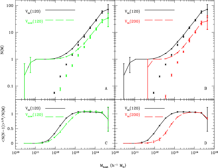
Figure 13.— Top: The average number of galaxies per host halo as a function of host halo mass. Bottom: Expression for the pairs per halo $<N(N-1)>^{1/2}/N(M)$ (relative to the Poisson expectation) as a function of host halo mass. In the upper panels, points with error bars reflect satellite galaxies and lines show the total (satellite plus central) galaxy count per halo. The left figure compares the $V_{\rm in}$ model (solid) and $V_{\rm now}$ model (dashed) using the same velocity cut to define the galaxy population (120 km s^-1). The right panel compares the $V_{\rm in}$ model at two different velocity cuts (120 and 200 km s^-1). The pair count per halo is well described by a Poisson distribution for the satellites and substantially sub-Poissonian for the central objects. Pair counts thus become important only for $N(M)\lower 2.58334pt\vbox{\hbox{$\buildrel\textstyle>\over{\sim}\ $}}2$, and will be dominated by massive halos.

On the other hand, for small separations, the number density of close pairs, $n_{p}$, will be dominated by pairs contained within single halos (Figure 3 illustrates that, for the $V_{\rm in}$ model, $\lower 2.58334pt\vbox{\hbox{$\buildrel\textstyle<\over{\sim}\ $}}10\%$ of close pairs reside in separate host halos according to typical close-pair definitions out to $z\leq 3$). Ignoring for the moment the precise velocity selection criteria, we can approximate the number density of pairs with physical projected separations meeting some range $r_{1}<r<r_{2}$ as

$$n_{\rm p}\simeq n_{\mathrm{p,1h}}=\frac{1}{2}\int_{M_{\rm min}}^{\infty}dM\frac{dn}{dM}\left<N(N-1)\right>_{M}F\left(r_{1,2}|M\right),$$ (7)

where $\left<N(N-1)\right>_{M}$ is the second moment of the HOD and $F(r_{1,2}|M)$ is the fraction of galaxy pairs that have projected separations between $r_{1}$ and $r_{2}$ within a dark matter halo of mass $M$. The function $F$ provides an $\sim$ order unity covering factor determined by the distribution of galaxies within halos . Notice that since $\left<N(N-1)\right>_{M}=N_{s}(M)^{2}$ and $N_{s}(M)\rightarrow 0$ for $M<M_{1}$, the pair number density $n_{p}$ (unlike $n_{g}$) explicitly selects against the mass regime dominated by “central galaxies” and favors halo with $M>M_{1}$.

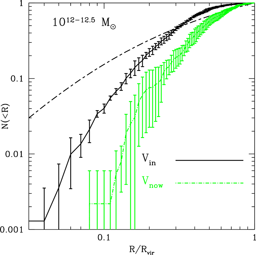
Figure 14.— The normalized cumulative number of satellite galaxies as a function of radius from the host halo center for host halos of mass $10^{12-12.25}h^{-1}M_{\odot}$ ($R_{\rm vir}\simeq 204h^{-1}{\rm kpc}$). The solid and dash-dot lines correspond to $V_{\rm in}$ and $V_{\rm now}=120$ km s^-1, respectively. The cumulative mass profile for a typical halo of this mass is shown by the dot-dash line. Error bars are RMS variations over the four Monte-Carlo subhalo realizations.

This simple and intuitive formalism immediately provides insight into the nature of the companion fraction, $N_{c}\equiv 2n_{\rm p}/n_{g}$. In the right-hand panel of Figure 12 we show the predicted value of $N_{c}$ vs. $n_{g}$ as calculated using the (approximate) equations 6 and 7 with $r_{1}=10h^{-1}{\rm kpc}$ and $r_{2}=50h^{-1}{\rm kpc}$ for several choices of HOD parameters defined in Equation 5. In all cases we assume that galaxies are distributed in dark matter halos following NFW profiles. The upper long-dashed line and solid line assume $M_{1}/M_{0}=10$ and $25$ respectively, use $p=1$ in the satellite $N_{s}(M)$ piece, and assume the NFW concentration-mass relation, $c(M)$, given in Bullock et al. (2001). The dot-dashed line is the same as the solid line except we fix the NFW concentration to a relatively low value, $c=5$, for all halos. Finally, the lower dashed line assumes $M_{1}/M_{0}=100$ with $p=1.2$ and the standard concentration relation.

From Figure 12 we see that as the size of the “plateau” region increases (characterized by increasing the ratio $M_{1}/M_{0}$) the galaxy number density is increasingly dominated by central galaxies and the pair fraction goes down. Also, even for a fixed HOD, $N_{c}$ decreases as galaxies are packed together more diffusely in halos (characterized by lowering $c$). Finally, as the satellite contribution steepens (higher $p$), $N_{c}$ increases at higher number densities because lower mass host halos begin to contain multiple galaxies.

As illustrated by this toy-model exploration, pair count statistics should provide an important constraint on galaxy HODs as well as the distribution of galaxies within halos. The constraint could prove particularly powerful when combined with larger-scale ($r\lower 2.58334pt\vbox{\hbox{$\buildrel\textstyle>\over{\sim}\ $}}100$ kpc) two-point correlation function constraints on the HOD. Correlation function constraints generally suffer a severe degeneracy between $P(N|M)$ and $F(r|M)$, but this degeneracy may be broken when coupled with close ($r\lower 2.58334pt\vbox{\hbox{$\buildrel\textstyle<\over{\sim}\ $}}50$ kpc) pair fraction constraints.

4.2. Discussion of Model Results

The halo model serves as a useful framework for discussing and explaining our simulation model results. Figure 13 shows the first and second moments of our simulation model HODs. The upper panels show $N(M)$ and the lower panel shows the number of pairs per halo compared to the Poisson expectation, $<N(N-1)>^{1/2}/<N>$. The left side of the figure shows how the HOD changes as we vary the selection criteria, with $V_{\rm in}>120$km s^-1subhalos represented by the solid line and $V_{\rm now}>120$km s^-1subhalos shown by the dashed line. As must be the case, the central galaxy term (analogous to $M_{0}$ in our toy example above) is unaffected by this choice, while the satellite component (points) is enhanced when galaxies are selected using $V_{\rm in}$. This has the effect of extending the “plateau” region in the $N(M)$ function and is qualitatively similar to increasing the $M_{1}/M_{0}$ ratio in our toy-model discussed above. In the right hand panel we show $N(M)$ for two different velocity cuts (120 compared to 200 km s^-1) both using $V_{\rm in}$ as the velocity of relevance. Here we see that both the satellite term and the central term are affected in this case ($M_{0}$ becomes larger as more massive satellites are selected). Note that as expected from the previous discussion of satellite vs. central galaxy statistics, the average number of pairs of galaxies per halo tracks the Poisson expectation for host masses where $N(M)\lower 2.58334pt\vbox{\hbox{$\buildrel\textstyle>\over{\sim}\ $}}2$ and becomes substantially sub-Poissonian for $N(M)\lower 2.58334pt\vbox{\hbox{$\buildrel\textstyle<\over{\sim}\ $}}2$. As discussed in reference to Equations 6 and 7, this means that while the total number density of galaxies (with, e.g., $V_{\rm in}\lower 2.58334pt\vbox{\hbox{$\buildrel\textstyle>\over{\sim}\ $}}120$km s^-1) will be dominated by host halos where $N(M)\simeq 1$ or with $M\simeq M_{0}\simeq 10^{11}h^{-1}M_{\odot}$, the total number density of close galaxy pairs will be dominated by much more massive host halos $M\lower 2.58334pt\vbox{\hbox{$\buildrel\textstyle>\over{\sim}\ $}}M_{1}\simeq 5\times 10^{12}h^{-1}M_{\odot}$ (where $N(M)\lower 2.58334pt\vbox{\hbox{$\buildrel\textstyle>\over{\sim}\ $}}2$).

In addition to its effect on $P(M|N)$, whether the galaxy light is more accurately traced by $V_{\rm now}$ or $V_{\rm in}$ will also affect the relative distribution of satellite galaxies within host halos. Recall that $V_{\rm now}$ selects “observable” galaxies based on a subhalo’s current maximum circular velocity and $V_{\rm in}$ selects galaxies based on the subhalos’ circular velocity when it was accreted into the system (these might mimic models where galaxies are more or less affected by mass loss or surface brightness dimming after accretion). As shown in Figure 14, the $V_{\rm in}$ selection results in a satellite galaxy distribution that is more centrally concentrated (and thus has more close pairs per halo) than does the $V_{\rm now}$ selected sample. The figure shows cumulative number of satellites relative to the total number of satellites as a function of radius, scaled to the virial radii of the hosts, from the host halo center using host halo masses of $M_{\rm vir}=10^{12-12.5}h^{-1}M_{\odot}$. The solid line shows this for the $V_{\rm in}$ case and the dashed line reflects the $V_{\rm now}$ case. For reference, the dot-dashed line above shows the cumulative mass distribution for a typical dark matter halo of this size (Bullock et al., 2001). The $V_{\rm now}$ case shows the effects of enhanced satellite destruction near the center. This difference certainly affects predictions for pair counts, however the main difference between $N_{c}$ counts in our two models is driven by the differences in their HODs.

Finally we turn to the evolution of the companion fraction with redshift. As discussed in the previous section, the average close companion count per galaxy is expected to evolve only weakly with redshift (e.g. Figure 4) and even declines at fixed comoving number density when pairs are identified within a fixed comoving separation (Figure 9). This occurs even though the merger rate per host dark matter halo increases at high redshift. This increase in merger rate is indeed reflected in the HOD. As shown in Figure 15, the average number of galaxies per halo at fixed host mass increases systematically at high redshift. However, from Equation 7, the number density of pairs depends both on the number of pairs per halo ($<N(N-1)>\sim N_{s}(M)^{2}$) and the number density of host halos ($dn/dM$). In Figure 15, for example, $N(M)$ is a factor of $\sim 2$ higher at $z\sim 3$ at the host mass where pair counts become non-negligible $M_{\rm host}\sim 10^{12}h^{-1}M_{\odot}$. However, host halos of this size are a factor of $\sim 5$ rarer at $z=3$ compared to $z=0$ (Figure 1). This results in a mild overall decline in the number of same halo pairs at high redshift.

The HOD formalism also helps us understand Figure 11, where we find that the average number of “Faint” galaxies per “Bright” galaxy increases more rapidly than does the “Bright-Bright” fraction with redshift. The more pronounced evolution comes about because “Faint” satellite selection decreases the characteristic host mass required for a satellite ($M_{1}\downarrow$). At the same time, we focus on “Bright” central galaxies, which keeps the minimum host halo mass for hosting a central galaxy ($M_{0}$) roughly fixed. As $M_{1}/M_{0}$ decreases, we are more likely to see an increased companion count (Figure 12).

5. Conclusions

In this paper we have investigated the use of close pair counts as a constraint on hierarchical structure formation using a model that combines a large ($120h^{-1}{\rm Mpc}$ box) $\Lambda$CDM N-body simulation (Allgood et al., 2006) with a rigorous analytic substructure code (Zentner et al., 2005) in order to achieve robust halo identification on small scales within a cosmologically-relevant volume. We measure close pairs in our simulation in exactly the same way they are observed in the real universe and use these close pair counts to test simple, yet physically well-motivated models for connecting galaxies with dark matter subhalos. We explore two models for the connection between galaxies and their associated dark matter subhalos: one in which satellite galaxy luminosities trace the current maximum circular velocities of their subhalos, $V_{\rm now}$, and a second in which a satellite galaxy’s luminosity is tightly correlated with the maximum circular velocity the subhalo had when it was first accreted into a host halo, $V_{\rm in}$. The latter case corresponds to a model where galaxies are much more resilient to mass loss than are their dark matter halos.

A highlighted summary of this work and our conclusions are as follows:

• We showed that $\Lambda$CDM models naturally reproduce the observed “weak” evolution in the close companion fraction, $N_{c}$, out to $z\sim 1.1$ as reported by the DEEP2 team (Lin et al., 2004). The result is driven by the fact that while merger rates (and the number of galaxy pairs per halo) increase towards high redshift, the number of halos massive enough to host a bright galaxy pair decreases with $z$.

• We used the SSRS2 and UZC surveys to derive companion counts as a function of the underlying galaxy population’s number density at $z=0$ and showed that the relatively high companion fraction observed favors a model where galaxies are more resistant to mass loss than are dark subhalos ($\sim$ the $V_{\rm in}$ model). Cosmic variance is unlikely to be qualitatively important in this conclusion, although verifying the result requires a complete redshift survey with a larger cosmic volume.

• We argued that the close luminous companion count per galaxy ($N_{c}$) does not track the distinct dark matter halo merger rate. Instead it tracks the luminous galaxy merger rate. While a direct connection between the two is often assumed, there is a mismatch because multiple galaxies may occupy the same host dark matter halo. The same arguments apply to morphological identifications of merger remnants, which also do not directly probe the host dark halo merger rate.

• We showed that while close pair statistics provide a poor direct constraint on halo merger rates, they provide an important constraint on the galaxy Halo Occupation Distribution (HOD). In this way, pair counts may act as a general tool for testing models of galaxy formation on $\lesssim 100$  kpc scales.

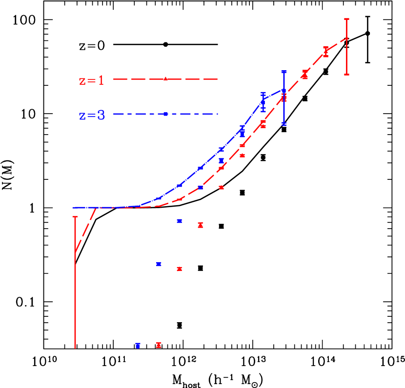
Figure 15.— The average number of galaxies per host dark matter halo with $V_{\rm in}>120$km s^-1shown at $z=0$, 1, and 3. The points reflect satellite halos while the lines include all galaxies.

Our results are not driven by the effects of false pair identification. We showed that standard techniques for identifying close pairs via close projected separations and line-of-sight velocity differences do quite well in identifying galaxy pairs which occupy the same dark matter halos (Figure 3). Typically $\lower 2.58334pt\vbox{\hbox{$\buildrel\textstyle>\over{\sim}\ $}}90\%$ of pairs identified in this manner occupy the same host dark matter halos out to a redshift of $\sim 2$ using the $V_{\rm in}$ model. It should be noted that this fraction does depend on the details of the association between subhalos and galaxies. The striking differences between our two toy models provides evidence of this. Typically, $\sim 20\%$ of pairs occupy different halos in the $V_{\rm now}$ model.

In conclusion, current close pair statistics are unable to rule out a simple scenario where galaxies are associated in a one-to-one way with dark matter subhalos (in particular our $V_{\rm in}$ association) in the current concordance $\Lambda$CDM  model. Better statistics, more complete surveys, and the ability to divide samples by color or stellar mass indicators will help refine this model and explore galaxy formation unknowns on $\lesssim 100$  kpc scales. Enumerating faint close companion counts around bright galaxies (Figure 11) will also provide a new and powerful test.

Appendix A Pair Fraction as a Function of Number Density

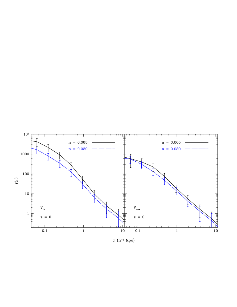
Figure 16.— Model $z=0$ correlation functions at two number densities. The left panel shows number densities defined using a cut on $V_{\rm now}$ and the right panel uses $V_{\rm in}$. Error-bars represent the quadrature sum of the standard deviation of the four model realizations and the cosmic variance computed by jackknife re-sampling of the eight octants of the volume.

One of the important findings in our analysis is that the observed companion fraction of galaxies should increase with the underlying galaxy number density (see, e.g. Figure 5). We can understand the tendency for $N_{c}$ to increase with $n_{g}$ at fixed redshift by considering the number of pairs expected in a fixed (physical) cylinder of volume $V$ (e.g., with length $\ell\simeq 2\Delta vH_{0}^{-1}\simeq 10h^{-1}$ Mpc and radius $r\simeq 50$ kpc). Let us start with the idealization of an uncorrelated sample. For an uncorrelated galaxy population, with mean number density $n_{g}$ in a large fiducial volume $V_{0}$, the total number of galaxies in the sample is clearly

$$N_{\rm gal}=n_{g}V_{0}.$$ (A1)

The average number of companions per galaxy is $N_{p}=n_{g}V$, so the number of companions in the entire sample is simply $n_{g}^{2}\,V\,V_{0}$. Therefore, for an unclustered galaxy population, the average number of companions per galaxy should increase linearly with galaxy number density,

$$N_{c}=n_{g}\,V\propto n_{g}.$$ (A2)

Extending this argument to the case of a clustered galaxy population is straightforward:

$$N_{p}=n_{g}V[1+\bar{\xi}],$$ (A3)

where $\bar{\xi}\equiv V^{-1}\int_{V}\xi(r){\rm d}V$ is the average of the correlation function over the volume of the cylinder. The total number of companions in the sample is then is $n_{g}^{2}[1+\bar{\xi}]VV_{0}$ and the companion fraction is

$$N_{c}=n_{g}V[1+\bar{\xi}]\approx n_{g}V\bar{\xi},$$ (A4)

where we assume $\xi(r)\gg 1$ at all relevant scales. There are both theoretical and direct observational reasons to believe that $\xi$ should increase with decreasing number density. If we take a simple power-law description $\bar{\xi}\propto n_{g}^{-\alpha}$ then we have

$$N_{c}\propto n_{g}^{1-\alpha}.$$ (A5)

Therefore, quite generally, as long as $\alpha<1$, the companion fraction should be an increasing function of galaxy number density.

The $z=0$ correlation function for our two simulation models at two characteristic galaxy number densities is shown in the left ($V_{\rm now}$) and right ($V_{\rm in}$) panels of Figure 16. Note that $\xi(r)$ at $r\lower 2.58334pt\vbox{\hbox{$\buildrel\textstyle<\over{\sim}\ $}}100$ $h^{-1}{\rm kpc}$ is quite flat for the $V_{\rm now}$ case but continues to rise for the $V_{\rm in}$ case. This reflects the enhanced “destruction” included in the $V_{\rm now}$ model (galaxies in the centers of halos tend to lose mass quickly and their $V_{\rm max}$ values drop out of the sample.) If we characterize the clustering vs. number density trend by fitting the amplitude of the $z=0$ correlation functions at $100h^{-1}{\rm kpc}$ with $\xi_{100}\propto n_{g}^{-\alpha}$ we find $\alpha\simeq 0.15$ for $V_{\rm now}$ and $\alpha\simeq 0.5$ for $V_{\rm in}$. From the above arguments with $\xi_{100}\approx\bar{\xi}$ we would then expect $N_{c}\propto n_{g}^{0.85}$ and $N_{c}\propto n_{g}^{0.5}$ for $V_{\rm now}$ and $V_{\rm in}$ respectively. Indeed, these are approximately the slopes measured at $z=0$ in Figure 5.

References

- Allgood et al. (2006) Allgood, B., Flores, R. A., Primack, J. R., Kravtsov, A. V., Wechsler, R. H., Faltenbacher, A., & Bullock, J. S. 2006, MNRAS, 367, 1781
- Azzaro et al. (2005) Azzaro, M., Zentner, A. R., Prada, F., & Klypin, A. 2005, ApJ, submitted; arXiv:astro-ph/0506547
- Barton et al. (2001) Barton, E. J., Geller, M. J., Bromley, B. C., van Zee, L., & Kenyon, S. J. 2001, AJ, 121, 625
- Barton et al. (2000) Barton, E. J., Geller, M. J., & Kenyon, S. J. 2000, ApJ, 530, 660
- Barton Gillespie et al. (2003) Barton Gillespie, E., Geller, M. J., & Kenyon, S. J. 2003, ApJ, 582, 668
- Bell et al. (2006) Bell, E. F., Phleps, S., Somerville, R. S., Wolf, C., Borch, A., & Meisenheimer, K. 2006, arXiv:astro-ph/0602038
- Berlind & Weinberg (2001) Berlind, A. & Weinberg, D. H. 2001, ApJ
- Blumenthal et al. (1984) Blumenthal, G. R., Faber, S. M., Primack, J. R., & Rees, M. J. 1984, Nature, 311, 517
- Bond et al. (1991) Bond, J. R., Cole, S., Efstathiou, G., & Kaiser, N. 1991, ApJ, 379, 440
- Bryan & Norman (1998) Bryan, G. L. & Norman, M. L. 1998, ApJ, 495, 80
- Bullock & Johnston (2005) Bullock, J. S. & Johnston, K. V. 2005, ApJ, 635, 931
- Bullock et al. (2001) Bullock, J. S., Kolatt, T. S., Sigad, Y., Somerville, R. S., Kravtsov, A. V., Klypin, A. A., Primack, J. R., & Dekel, A. 2001, MNRAS, 321, 559
- Bullock et al. (2000) Bullock, J. S., Kravtsov, A. V., & Weinberg, D. 2000, ApJ, 539, 517
- Bullock et al. (2002) Bullock, J. S., Wechsler, R. H., & Somerville, R. S. 2002, MNRAS, 329, 246
- Bundy et al. (2004) Bundy, K., Fukugita, M., Ellis, R. S., Kodama, T., & Conselice, C. J. 2004, ApJ, 601, L123
- Burkey et al. (1994) Burkey, J. M., Keel, W. C., Windhorst, R. A., & Franklin, B. E. 1994, ApJ, 429, L13
- Carlberg et al. (1994) Carlberg, R. G., Pritchet, C. J., & Infante, L. 1994, ApJ, 435, 540
- Carlberg et al. (2000) Carlberg, R. G. et al. 2000, ApJ, 532, L1
- Chandrasekhar (1943) Chandrasekhar, S. 1943, ApJ, 97, 255
- Conroy et al. (2006) Conroy, C., Wechsler, R. H., & Kravtsov, A. V. 2006, ApJ, in press; arXiv:astro-ph/0512234
- Conselice et al. (2003) Conselice, C. J., Bershady, M. A., Dickinson, M., & Papovich, C. 2003, AJ, 126, 1183
- Cooray & Milosavljević (2005) Cooray, A. & Milosavljević, M. 2005, ApJ, 627, L85
- Diemand et al. (2004) Diemand, J., Moore, B., & Stadel, J. 2004, MNRAS, 352, 535
- Dressler (1980) Dressler, A. 1980, ApJ, 236, 351
- Falco et al. (1999) Falco, E. E., Kurtz, M. J., Geller, M. J., Huchra, J. P., Peters, J., Berlind, P., Mink, D. J., Tokarz, S. P., & Elwell, B. 1999, VizieR Online Data Catalog, 611, 10438
- Faltenbacher & Diemand (2006) Faltenbacher, A. & Diemand, J. 2006, MNRAS, 566, arXiv:astro-ph/0602197
- Fasano (1984) Fasano, G. 1984, Memorie della Societa Astronomica Italiana, 55, 457
- Gao et al. (2004) Gao, L., De Lucia, G., White, S. D. M., & Jenkins, A. 2004, MNRAS, 352, L1
- Geller & Huchra (1989) Geller, M. J. & Huchra, J. P. 1989, Science, 246, 897
- Giovanelli & Haynes (1985) Giovanelli, R. & Haynes, M. P. 1985, AJ, 90, 2445
- Giovanelli & Haynes (1989) —. 1989, AJ, 97, 633
- Giovanelli & Haynes (1993) —. 1993, AJ, 105, 1271
- Giovanelli et al. (1986) Giovanelli, R., Myers, S. T., Roth, J., & Haynes, M. P. 1986, AJ, 92, 250
- Gottlöber et al. (2001) Gottlöber, S., Klypin, A., & Kravtsov, A. V. 2001, ApJ, 546, 223
- Governato et al. (1999) Governato, F., Gardner, J. P., Stadel, J., Quinn, T., & Lake, G. 1999, AJ, 117, 1651
- Hashimoto et al. (2003) Hashimoto, Y., Funato, Y., & Makino, J. 2003, ApJ, 582, 196
- Haynes et al. (1988) Haynes, M. P., Magri, C., Giovanelli, R., & Starosta, B. M. 1988, AJ, 95, 607
- Holmberg (1937) Holmberg, E. 1937, Annals of the Observatory of Lund, 6, 1
- Huchra et al. (1995) Huchra, J. P., Geller, M. J., & Corwin, H. G. 1995, ApJS, 99, 391
- Huchra et al. (1990) Huchra, J. P., Geller, M. J., de Lapparent, V., & Corwin, H. G. 1990, ApJS, 72, 433
- Kauffmann et al. (1993) Kauffmann, G., White, S. D. M., & Guiderdoni, B. 1993, MNRAS, 264, 201
- Kazantzidis et al. (2004) Kazantzidis, S., Mayer, L., Mastropietro, C., Diemand, J., Stadel, J., & Moore, B. 2004, ApJ, 608, 663
- Kennicutt & Keel (1984) Kennicutt, R. C. & Keel, W. C. 1984, ApJ, 279, L5
- Klypin et al. (1999) Klypin, A., Gottlöber, S., Kravtsov, A. V., & Khokhlov, A. M. 1999, ApJ, 516, 530
- Kolatt et al. (1999) Kolatt, T. S., Bullock, J. S., Somerville, R. S., Sigad, Y., Jonsson, P., Kravtsov, A. V., Klypin, A. A., Primack, J. R., Faber, S. M., & Dekel, A. 1999, ApJ, 523, L109
- Kravtsov et al. (2004a) Kravtsov, A. V., Berlind, A. A., Wechsler, R. H., Klypin, A. A., Gottlöber, S., Allgood, B., & Primack, J. R. 2004a, ApJ, 609, 35
- Kravtsov et al. (2004b) Kravtsov, A. V., Gnedin, O. Y., & Klypin, A. A. 2004b, ApJ, 609, 482
- Kravtsov et al. (1997) Kravtsov, A. V., Klypin, A. A., & Khokhlov, A. M. 1997, ApJS, 111, 73
- Lacey & Cole (1993) Lacey, C. & Cole, S. 1993, MNRAS, 262, 627
- Larson & Tinsley (1978) Larson, R. B. & Tinsley, B. M. 1978, ApJ, 219, 46
- Le Fèvre et al. (2000) Le Fèvre, O. et al. 2000, MNRAS, 311, 565
- Lin et al. (2004) Lin, L. et al. 2004, ApJ, 617, L9
- Lotz et al. (2006) Lotz, J. M. et al. 2006, arXiv:astro-ph/0602088
- Maller et al. (2005) Maller, A., Katz, N., Keres, D., Dave, R., & Weinberg, D. H. 2005, ApJ, submitted; arXiv:astro-ph/0509474
- Marzke et al. (1998) Marzke, R. O., da Costa, L. N., Pellegrini, P. S., Willmer, C. N. A., & Geller, M. J. 1998, ApJ, 503, 617
- Marzke et al. (1994) Marzke, R. O., Huchra, J. P., & Geller, M. J. 1994, ApJ, 428, 43
- Masjedi et al. (2005) Masjedi, M. et al. 2005, arXiv:astro-ph/0512166
- Nagai & Kravtsov (2005) Nagai, D. & Kravtsov, A. V. 2005, ApJ, 618, 557
- Navarro et al. (1997) Navarro, J. F., Frenk, C. S., & White, S. D. M. 1997, ApJ, 490, 493
- Neuschaefer et al. (1997) Neuschaefer, L. W., Im, M., Ratnatunga, K. U., Griffiths, R. E., & Casertano, S. 1997, ApJ, 480, 59
- Patton et al. (2000) Patton, D. R., Carlberg, R. G., Marzke, R. O., Pritchet, C. J., da Costa, L. N., & Pellegrini, P. S. 2000, ApJ, 536, 153
- Patton et al. (1997) Patton, D. R., Pritchet, C. J., Yee, H. K. C., Ellingson, E., & Carlberg, R. G. 1997, ApJ, 475, 29
- Patton et al. (2002) Patton, D. R. et al. 2002, ApJ, 565, 208
- Peñarrubia & Benson (2005) Peñarrubia, J. & Benson, A. J. 2005, MNRAS, 364, 977
- Peacock & Smith (2000) Peacock, J. A. & Smith, R. E. 2000, MNRAS, 318, 1144
- Postman & Geller (1984) Postman, M. & Geller, M. J. 1984, ApJ, 281, 95
- Scoccimarro et al. (2001) Scoccimarro, R., Sheth, R. K., Hui, L., & Jain, B. 2001, ApJ, 546, 20
- Seljak (2000) Seljak, U. 2000, MNRAS, 318, 203
- Somerville & Kolatt (1999) Somerville, R. S. & Kolatt, T. S. 1999, MNRAS, 305, 1
- Tasitsiomi et al. (2004) Tasitsiomi, A., Kravtsov, A. V., Wechsler, R. H., & Primack, J. R. 2004, ApJ, 614, 533
- Taylor & Babul (2004) Taylor, J. E. & Babul, A. 2004, MNRAS, 348, 811
- Tinker et al. (2005) Tinker, J. L., Weinberg, D. H., Zheng, Z., & Zehavi, I. 2005, ApJ, 631, 41
- Toomre & Toomre (1972) Toomre, A. & Toomre, J. 1972, ApJ, 178, 623
- Tully & Fisher (1977) Tully, R. B. & Fisher, J. R. 1977, A&A, 54, 661
- van den Bosch et al. (2005) van den Bosch, F. C., Tormen, G., & Giocoli, C. 2005, MNRAS, 359, 1029
- Wang et al. (2006) Wang, L., Li, C., Kauffmann, G., & De Lucia, G. 2006, astro-ph/0603646
- Wechsler et al. (2002) Wechsler, R. H., Bullock, J. S., Primack, J. R., Kravtsov, A. V., & Dekel, A. 2002, ApJ, 568, 52
- Wechsler et al. (2001) Wechsler, R. H., Somerville, R. S., Bullock, J. S., Kolatt, T. S., Primack, J. R., Blumenthal, G. R., & Dekel, A. 2001, ApJ, 554, 1
- Wechsler et al. (2006) Wechsler, R. H., Zentner, A. R., Bullock, J. S., Kravtsov, A. V., & Allgood, B. 2006, ApJ, in press, arXiv:astro-ph/0512416
- Wegner et al. (1993) Wegner, G., Haynes, M. P., & Giovanelli, R. 1993, AJ, 105, 1251
- Weinberg et al. (2006) Weinberg, D. H., Colombi, S., Davé, R., & Katz, N. 2006, ApJ, submitted
- Woods et al. (1995) Woods, D., Fahlman, G. G., & Richer, H. B. 1995, ApJ, 454, 32
- Yee & Ellingson (1995) Yee, H. K. C. & Ellingson, E. 1995, ApJ, 445, 37
- Zentner et al. (2005) Zentner, A. R., Berlind, A. A., Bullock, J. S., Kravtsov, A. V., & Wechsler, R. H. 2005, ApJ, 624, 505
- Zentner & Bullock (2003) Zentner, A. R. & Bullock, J. S. 2003, ApJ, 598, 49
- Zepf & Koo (1989) Zepf, S. E. & Koo, D. C. 1989, ApJ, 337, 34