Black-Hole Accretion Disc as an Analogue Gravity Model

Abstract

We formulate and solve the equations governing the transonic behaviour of a general relativistic black-hole accretion disc with non-zero advection velocity. We demonstrate that a relativistic Rankine-Hugoniot shock may form leading to the formation of accretion powered outflow. We show that the critical points of transonic discs generally do not coincide with the corresponding sonic points. The collection of such sonic points forms an axisymmetric hypersurface, generators of which are the acoustic null geodesics, i.e. the phonon trajectories. Such a surface is shown to be identical with an acoustic event horizon. The acoustic surface gravity and the corresponding analogue horizon temperature $T_{AH}$ at the acoustic horizon are then computed in terms of fundamental accretion parameters. Physically, the analogue temperature is associated with the thermal phonon radiation analogous to the Hawking radiation of the black-hole horizon.Thus, an axisymmetric black-hole accretion disc is established as a natural example of the classical analogue gravity model, for which two kinds of horizon exist simultaneously. We have shown that for some values of astrophysically relevant accretion parameters, the analogue temperature exceeds the corresponding Hawking temperature. We point out that acoustic white holes can also be generated for a multi-transonic black-hole accretion with a shock. Such a white hole, produced at the shock, is always flanked by two acoustic black holes generated at the inner and the outer sonic points. Finally, we discuss possible applications of our work to other astrophysical events which may exhibit analogue effects.

I Introduction

I.1 Black-hole analogue

In recent years, strong analogies have been established between the physics of acoustic perturbations in an inhomogeneous dynamical fluid system, and some kinematic features of space-time in general relativity. An effective metric, referred to as the ‘acoustic metric’, which describes the geometry of the manifold in which acoustic perturbations propagate, can be constructed. This effective geometry can capture the properties of curved space-time in general relativity. Physical models constructed utilizing such analogies are called ‘analogue gravity models’ (for details on analogue gravity models, see, e.g. the review articles barcelo ; cardoso , and the book novello ).

One of the most significant effects of analogue gravity is the ‘classical black-hole analogue’. Classical black-hole analogue effects may be observed when acoustic perturbations (sound waves) propagate through a classical, dissipationless, inhomogeneous transonic fluid. Any acoustic perturbation, dragged by a supersonically moving fluid, can never escape upstream by penetrating the ‘sonic surface’. Such a sonic surface is a collection of transonic points in space-time, and can act as a ‘trapping’ surface for outgoing phonons. Hence, the sonic surface is actually an acoustic horizon, which resembles a black-hole event horizon in many ways and is generated at the transonic point in the fluid flow. The acoustic horizon is essentially a null hyper surface, generators of which are the acoustic null geodesics, i.e. the phonons. The acoustic horizon emits acoustic radiation with quasi thermal phonon spectra, which is analogous to the actual Hawking radiation. The temperature of the radiation emitted from the acoustic horizon is referred to as the analogue Hawking temperature.

In his pioneering work, Unruh unruh showed that the scalar field describing the acoustic perturbations in a transonic barotropic irrotational fluid, satisfied a Klein-Gordon type differential equation for the massless scalar field propagating in curved space-time with a metric that closely resembles the Schwarzschild metric near the horizon. The acoustic propagation through a transonic fluid forms an analogue event horizon located at the transonic point. Acoustic waves with a quasi thermal spectrum will be emitted from the acoustic horizon and the temperature of such acoustic radiation is given by unruh

$$T_{\rm AH}=\frac{\hbar}{4{\pi}\kappa_{\rm B}}\left[\frac{1}{c_{s}}\frac{{\partial}{u_{\perp}^{2}}}{\partial{\eta}}\right]_{\rm Acoustic~{}Horizon}\,,$$ (1)

where $\kappa_{\rm B}$ is Boltzmann’s constant, ${\hbar}$ is the Planck constant devided by $2\pi$, $c_{s}$ the speed of sound, $u_{\perp}$ the component of the flow velocity normal to the acoustic horizon and $\partial/\partial{\eta}$ represents the normal derivative. The temperature $T_{\rm AH}$ defined by Eq. (1) is the acoustic analogue of the usual Hawking temperature $T_{\rm H}$:

$$T_{\rm H}=\frac{{\hbar}c^{3}}{8{\pi}\kappa_{\rm B}GM_{\rm bh}}$$ (2)

and hence $T_{\rm AH}$ is referred to as the analogue Hawking temperature. In eq. (2), $M_{bh}$ is the black-hole mass, $G$ Newton’s gravitational constant, $c$ the velocity of light in the vacuum. Note that the sound speed in Eq. (1) in Unruh’s original treatment unruh was assumed constant in space.

Unruh’s work unruh was followed by other important papers jacob ; 95unruh ; visser ; 99jacob ; bilic . A more general treatment of the classical analogue radiation for Newtonian fluid was discussed by Visser visser who considered a general barotropic, inviscid fluid. The acoustic metric for a point sink was shown to be conformally related to the Painlevé-Gullstrand-Lemaître form of the Schwarzschild metric and a more general expression for analogue temperature was obtained, where unlike Unruh’s original expression unruh , the speed of sound was allowed to depend on space coordinates. In order to determine the analogue Hawking temperature of a classical analogue system, one needs to know the location of the acoustic horizon, the velocity of the fluid and the speed of sound and their space gradients at the acoustic horizon.

In the analogue gravity systems discussed above, the fluid flow is non-relativistic in flat Minkowski space, whereas the sound wave propagating through the non-relativistic fluid is coupled to a curved pseudo-Riemannian metric. This approach has been extended to relativistic fluids bilic by incorporating the general relativistic dynamics of the fluid flow. Since the introduction of viscosity may destroy Lorenz invariance, the acoustic analogue is best studied in a vorticity free dissipationless fluid.

I.2 Transonic accretion as a black-hole analogue: the motivation.

The process by which any gravitating, massive, astrophysical object captures its surrounding fluid is called accretion. If $c_{s}(r)$ is the local speed of sound and $u(r)$ is the instantaneous radial velocity of the accreting fluid, moving along a space curve parameterized by $r$, then the local Mach number of the fluid can be defined as $M(r)=u(r)/c_{s}(r)$. The flow will be locally subsonic or supersonic, according to $M(r)<1$ or $M(r)>1$, i.e. according to $u(r)<c_{s}(r)$ or $u(r)>c_{s}(r)$. The flow is transonic if at any moment it crosses $M=1$. This happens when a subsonic to supersonic or a supersonic to subsonic transition takes place either continuously or discontinuously. The points where such crossing takes place continuously are called sonic points, and the points of discontinuous transition are called shocks or discontinuities.

If the accreting material is assumed to be at rest far from the black hole, the flow must exhibit transonic behaviour in order to satisfy the inner boundary conditions imposed by the event horizon. Since the publication of the seminal paper by Bondi in 1952 bondi , the transonic behaviour of accreting fluid onto compact astrophysical objects has been extensively studied in the astrophysics community. Similarly, Unruh’s paper unruh initiated a substantial number of works in the theory of analogue Hawking effects with diverse fields of application novello ; barcelo . However, except for Moncrief monc and Anderson anderson , until recently no attempt was made to bridge the astrophysical black-hole accretion and the theory of analogue Hawking radiation, by providing a self-consistent study of analogue Hawking radiation for real astrophysical fluid flows, i.e. by establishing the fact that accreting black holes can be considered as a natural example of analogue system. Since both the theory of transonic astrophysical accretion and the theory of analogue Hawking radiation are based on general relativity, it is almost self-evident that accreting black holes can be considered as a natural example of analogue system.

Motivated by the above mentioned arguments, it has recently been shown dascqg ; topu that a spherically accreting astrophysical black-hole system is a unique example of classical analogue gravity model which exhibits both the black-hole event horizon and the analog acoustic horizon. Hence, an accreting astrophysical black hole may be considered an ideal candidate to study these two different types of horizons theoretically and to compare their properties.

Analogue effects in an idealized axisymmetric system have recently been investigated abraham . There, the axisymmetric astrophysical accretion has been modelled by a rotating fluid disc of constant thickness with the distribution of matter in the disc independent of the $z$ coordinate along the axis of rotation. In this paper, we study analogue effects in a more realistic astrophysical system in which the accretion disc thickness is calculated by solving the relativistic Euler equation in the vertical direction. The expression for the local disc height obtained in this way is a function of the local fluid velocity, the local speed of sound and the space coordinate $r$. As will be shown in section II.6, in our realistic disc model, in contrast to the disc with constant thickness, the sonic points do not coincide with the critical points, and the overall picture may also differ from that in abraham .

In the following sections, we describe how to model a general relativistic, axially symmetric, multi-transonic flow of perfect fluid accreting onto astrophysical black holes. We formulate and solve the basic equations in section II, and then explore the transonic behaviour of the flow in section III. In section IV we show that a relativistic standing shock wave can form in the accretion disc if the flow is potentially multi-transonic. We discuss the relevant acoustic geometry in detail in section V. In section VI, we show how to calculate the analogue Hawking temperature. Finally, we conclude the paper with section VII.

II Transonic black-hole accretion disc in general relativity

II.1 Multi-transonic flow

For the flow of matter with non-zero angular momentum density, accretion phenomena are studied employing axisymmetric configuration. Accreting matter is thrown into circular orbits around the central accretor, leading to the formation of accretion discs. The pioneering contribution to study the properties of general relativistic black-hole accretion discs may be attributed to two classic papers bardeen ; nt73 . For certain values of the intrinsic angular momentum density of accreting material, the number of sonic points, unlike in spherical accretion, may exceed one, and accretion is called ‘multi-transonic’. The study of multi-transonic flow was initiated by Abramowicz and Zurek zurek . Subsequently, multi-transonic behaviour in black-hole accretion discs have been expansively studied matsumoto ; lu ; bozena ; fukue ; kato ; sandy ; kafatos ; pariev ; peitz ; luetal ; apj1 ; mnras4 . Typically, the outermost sonic point lies close to the corresponding Bondi radius. The innermost sonic point and the middle sonic point exist within and outside the marginally stable orbit, respectively, for the general relativistic as well as for the post-Newtonian model of accretion flow. The location of the sonic points can be calculated as a function of the specific flow energy ${\cal E}$ (Bernoulli’s constant), the specific angular momentum $\lambda$ and the inflow polytropic index $\gamma$. The literature on multi-transonic flow usually deals with low angular momentum accretion flow. Sub-Keplerian weakly rotating flows are exhibited in various physical situations, such as detached binary systems fed by accretion from the so-called OB stellar winds ilashu ; liang , semi-detached low-mass non-magnetic binaries bisikalo , and super-massive black holes fed by accretion from slowly rotating central stellar clusters ila ; ho . Even for a standard Keplerian accretion disc, turbulence may produce such low angular momentum flow (see, e.g. igu and references therein).

II.2 The dynamics

For the most general description of fluid flow in strong gravity, one needs to solve the equations of motion for the fluid and the Einstein equations. The problem may be simplified by assuming the accretion to be non-self-gravitating, so that the fluid dynamics may be dealt with in a metric without back-reactions. We use the units $G=c=M_{bh}=1$, so that radial distances and velocities are scaled in units $r_{g}\equiv\frac{G{M_{bh}}}{c^{2}}$ and $c$, respectively, and all other derived quantities are scaled accordingly.

We use the Boyer-Lindquist coordinates boyer with signature $-+++$, and an azimuthally Lorentz boosted orthonormal tetrad basis corotating with the accreting fluid. We define $\lambda$ to be the specific angular momentum of the flow and neglect any gravo-magneto-viscous non-alignment between $\lambda$ and the black-hole spin angular momentum.

Let $v_{\mu}$ be the four velocity of the (perfect) accreting fluid. The energy momentum tensor ${T}^{{\mu}{\nu}}$ is then given by

$${T}_{{\mu}{\nu}}=\left(\epsilon+p\right)v_{\mu}v_{\nu}+pg_{{\mu}{\nu}},$$ (3)

with $\epsilon$ and $p$ being the fluid energy density and pressure, respectively.

In this paper, we study the inviscid accretion of hydrodynamic fluid. Hence, our calculation will be focused on the stationary axisymmetric solution of the energy momentum and baryon number conservation equations

$${T^{{\mu}{\nu}}}_{;\nu}=0;\;\;\;\;\;\left({\rho}{v^{\mu}}\right)_{;\mu}=0,$$ (4)

where $\rho$ is the rest-mass density. Specifying the metric to be stationary and axially symmetric, the two generators $\xi^{\mu}\equiv(\partial/\partial t)^{\mu}$ and $\phi^{\mu}\equiv(\partial/\partial\phi)^{\mu}$ of the temporal and axial isometry, respectively, are Killing vectors.

We consider the flow to be ‘advective’, i.e. to possess considerable radial three-velocity. The above-mentioned advective velocity, which we hereafter denote by $u$ and consider it to be confined on the equatorial plane, is essentially the three-velocity component perpendicular to the set of hypersurfaces $\{\Sigma_{v}\}$ defined by $v^{2}=const$, where $v$ is the magnitude of the 3-velocity. Each $\Sigma_{v}$ is timelike since its normal $\eta_{\mu}\propto\partial_{\mu}v^{2}$ is spacelike and may be normalized as $\eta^{\mu}\eta_{\mu}=1$.

We then define the specific angular momentum $\lambda$ and the angular velocity $\Omega$ as

$$\lambda=-\frac{v_{\phi}}{v_{t}};\;\;\;\;\;\Omega=\frac{v^{\phi}}{v^{t}}=-\frac{g_{t\phi}+\lambda{g}_{tt}}{{g_{\phi{\phi}}+\lambda{g}_{t{\phi}}}}\,,$$ (5)

The metric on the equatorial plane is given by nt73

$$ds^{2}=g_{{\mu}{\nu}}dx^{\mu}dx^{\nu}=-\frac{r^{2}{\Delta}}{A}dt^{2}+\frac{A}{r^{2}}\left(d\phi-\omega{dt}\right)^{2}+\frac{r^{2}}{\Delta}dr^{2}+dz^{2},$$ (6)

where $\Delta=r^{2}-2r+a^{2},~{}A=r^{4}+r^{2}a^{2}+2ra^{2}$, and $\omega=2ar/A$, $a$ being the Kerr parameter related to the black-hole spin. The normalization condition $v^{\mu}{v}_{\mu}=-1$, together with the expressins for $\lambda$ and $\Omega$ in Eq. (5), provides the relationship between the advective velocity $u$ and the temporal component of the four velocity

$$v_{t}=\left[\frac{Ar^{2}\Delta}{\left(1-u^{2}\right)\left\{A^{2}-4\lambda arA+\lambda^{2}r^{2}\left(4a^{2}-r^{2}\Delta\right)\right\}}\right]^{1/2}.$$ (7)

II.3 Thermodynamics

In order to solve Eqs. (4), we need to specify a realistic equation of state. In this work, we concentrate on polytropic accretion. However, polytropic accretion is not the only choice to describe the general relativistic transonic black-hole accretion. Equations of state other than the adiabatic one, such as the isothermal equation kafatos or the two-temperature plasma manmoto , have also been used to study the black-hole accretion flow.

We assume the dynamical in-fall time scale to be short compared with any dissipation time scale during the accretion process. To describe the fluid, we use a polytropic equation of state of the form

$$p=K{\rho}^{\gamma},$$ (8)

where the polytropic index $\gamma$ equal to the ratio of the two specific heats $c_{p}$ and $c_{v}$ of the accreting material is assumed to be constant throughout the fluid. A more realistic model of the flow would perhaps require a variable polytropic index having a functional dependence on the radial distance, i.e. $\gamma=\gamma(r)$. However, we have performed the calculations for a sufficiently large range of $\gamma$ and we believe that all astrophysically relevant polytropic indices are covered.

The constant $K$ in Eq. (8) may be related to the specific entropy of the fluid, provided there is no entropy generation during the flow. If in addition to (8) the Clapeyron equation for an ideal gas holds

$$p=\frac{\kappa_{B}}{{\mu}m_{p}}{\rho}T\,,$$ (9)

where $T$ is the locally measured temperature, $\mu$ the mean molecular weight, $m_{H}{\sim}m_{p}$ the mass of the hydrogen atom, then the specific entropy, i.e. the entropy per particle, is given by landau

$$\sigma=\frac{1}{\gamma-1}\log K+\frac{\gamma}{\gamma-1}+{\rm constant},$$ (10)

where the constant depends on the chemical composition of the accreting material. Equation (10) confirms that $K$ in Eq. (8) is a measure of the specific entropy of the accreting matter.

The specific enthalpy of the accreting matter can now be defined as

$$h=\frac{\left(p+\epsilon\right)}{\rho}\,,$$ (11)

where the energy density $\epsilon$ includes the rest-mass density and the internal energy and may be written as

$$\epsilon=\rho+\frac{p}{\gamma-1}\,.$$ (12)

The adiabatic speed of sound is defined by

$$c_{s}^{2}=\frac{{\partial}p}{{\partial}{\epsilon}}{\Bigg{|}}_{\rm constant~{}entropy}\,.$$ (13)

From Eq. (12) we obtain

$$\frac{\partial{\rho}}{\partial{\epsilon}}=\left(\frac{\gamma-1-c_{s}^{2}}{\gamma-1}\right).$$ (14)

Combination of Eq. (13) and Eq. (8) gives

$$c_{s}^{2}=K{\rho}^{\gamma-1}{\gamma}\frac{\partial{\rho}}{\partial{\epsilon}}\,,$$ (15)

Using the above relations, one obtains the expression for the specific enthalpy

$$h=\frac{\gamma-1}{\gamma-1-c_{s}^{2}}\,.$$ (16)

The rest-mass density $\rho$, the pressure $p$, the temperature $T$ of the flow and the energy density $\epsilon$ may be expressed in terms of the speed of sound $c_{s}$ as

$$\rho=K^{-\frac{1}{\gamma-1}}\left(\frac{\gamma-1}{\gamma}\right)^{\frac{1}{\gamma-1}}\left(\frac{c_{s}^{2}}{\gamma-1-c_{s}^{2}}\right)^{\frac{1}{\gamma-1}},$$ (17)

$$p=K^{-\frac{1}{\gamma-1}}\left(\frac{\gamma-1}{\gamma}\right)^{\frac{\gamma}{\gamma-1}}\left(\frac{c_{s}^{2}}{\gamma-1-c_{s}^{2}}\right)^{\frac{\gamma}{\gamma-1}},$$ (18)

$$T=\frac{\kappa_{B}}{{\mu}m_{p}}\left(\frac{\gamma-1}{\gamma}\right)\left(\frac{c_{s}^{2}}{\gamma-1-c_{s}^{2}}\right),$$ (19)

$$\epsilon=K^{-\frac{1}{\gamma-1}}\left(\frac{\gamma-1}{\gamma}\right)^{\frac{1}{\gamma-1}}\left(\frac{c_{s}^{2}}{\gamma-1-c_{s}^{2}}\right)^{\frac{1}{\gamma-1}}\left[1+\frac{1}{\gamma}\left(\frac{c_{s}^{2}}{\gamma-1-c_{s}^{2}}\right)\right].$$ (20)

II.4 Disc geometry and conservation equations

We assume that the disc has a radius-dependent local thickness $H$, and its central plane coincides with the equatorial plane of the black hole. It is a standard practice in accretion disc theory to use the vertically integrated model in describing the black-hole accretion discs where the equations of motion apply to the equatorial plane of the black hole, assuming the flow to be in hydrostatic equilibrium in the transverse direction. We follow the same procedure here. The flow variables are averaged over the disc height, i.e. a quantity $y$ used in our model is vertically integrated over the disc height and averaged as $\bar{y}=\int^{H}_{0}dh\,y/H$. We follow discheight to derive an expression for the disc height $H$ in our flow geometry since the relevant equations in discheight are non-singular on the horizon and can accommodate both the axial and a quasi-spherical flow geometry. In the Newtonian framework, the disc height in vertical equilibrium is obtained from the $z$ component of the non-relativistic Euler equation where all the terms involving velocities and the higher powers of $\left(({z}/{r}\right)$ are neglected. In the case of a general relativistic disc, the vertical pressure gradient in the comoving frame is compensated by the tidal gravitational field. We then obtain the disc height

$$H=\sqrt{\frac{2}{\gamma+1}}r^{2}\left[\frac{(\gamma-1)c^{2}_{c}}{\{\gamma-(1+c^{2}_{s})\}\{\lambda^{2}v_{t}^{2}-a^{2}(v_{t}-1)\}}\right]^{\frac{1}{2}},$$ (21)

which, by making use of Eq. (7), may be be expressed in terms of the advective velocity $u$.

The temporal component of the energy momentum tensor conservation equation leads to the constancy along each streamline of the flow specific energy ${\cal E}$ (relativistic analogue of Bernoulli’s constant) defined as anderson

$${\cal E}=hv_{t}.$$ (22)

From (7) and (16) it follows

$${\cal E}=\left[\frac{(\gamma-1)}{\gamma-(1+c^{2}_{s})}\right]\sqrt{\left(\frac{1}{1-u^{2}}\right)\left[\frac{Ar^{2}\Delta}{A^{2}-4\lambda arA+\lambda^{2}r^{2}(4a^{2}-r^{2}\Delta)}\right]}\,.$$ (23)

The rest-mass accretion rate ${\dot{M}}$ is obtained by integrating the relativistic continuity equation (4). One finds

$${\dot{M}}=4{\pi}{\Delta}^{\frac{1}{2}}H{\rho}\frac{u}{\sqrt{1-u^{2}}}\,,$$ (24)

Here, we adopt the sign convention that a positive $u$ corresponds to accretion. The entropy accretion rate ${\dot{S}}$ is a quasi-constant multiple of the mass accretion rate:

$${\dot{S}}=\left(\frac{1}{\gamma}\right)^{\left(\frac{1}{\gamma-1}\right)}4\pi\Delta^{\frac{1}{2}}c_{s}^{\left(\frac{2}{\gamma-1}\right)}\frac{u}{\sqrt{1-u^{2}}}\left[\frac{(\gamma-1)}{\gamma-(1+c^{2}_{s})}\right]^{\left(\frac{1}{\gamma-1}\right)}H.$$ (25)

Note that, in the absence of creation or annihilation of matter, the mass accretion rate is a constant of motion, whereas the entropy accretion rate is not. As the expression for ${\dot{S}}$ contains the quantity $K\equiv p/\rho^{\gamma}$, which measures the specific entropy of the flow, the entropy rate ${\dot{S}}$ remains constant throughout the flow only if the entropy per particle remains locally unchanged. This latter condition may be violated if the accretion is accompanied by a shock. Thus, ${\dot{S}}$ is a constant of motion for shock-free polytropic accretion and becomes discontinuous (increases) at the shock location, if a shock forms in the accretion. One can solve the two conservation equations for ${\cal E}$ and ${\dot{S}}$ to obtain the complete accretion profile. In this paper, we concentrate on the Schwarzschild metric only. A more general solution for the Kerr metric is in progress and will be presented elsewhere. For $a=0$, the expressions for ${\cal E}$, ${\dot{M}}$ and ${\dot{S}}$ are

$${\cal E}_{\rm Schwarzschild}=\left[\frac{(\gamma-1)}{\gamma-(1+c^{2}_{s})}\right]r\sqrt{\frac{r-2}{r^{3}-\lambda^{2}\left(r-2\right)}}\frac{1}{\sqrt{1-u^{2}}},$$ (26)

$$\dot{M}_{\rm Schwarzschild}=\frac{4{\pi}{\rho}c_{s}r^{\frac{3}{2}}u}{\lambda}\sqrt{\frac{2\left(\gamma-1\right)\left[r^{3}-\lambda^{2}\left(r-2\right)\right]}{\gamma\left[\gamma-\left(1+c_{s}^{2}\right)\right]}}\,,$$ (27)

$${\dot{S}}_{\rm Schwarzschild}=4\pi\left(\frac{1}{\lambda}\sqrt{\frac{2}{\gamma}}\right)\left[\frac{c_{s}}{\left(1-\frac{c_{s}^{2}}{\gamma-1}\right)^{\frac{1}{2}}}\right]^{\frac{\gamma+1}{\gamma-1}}ur\left[r^{4}-\lambda^{2}r(r-2)\right]^{\frac{1}{2}},$$ (28)

The corresponding disc height is given by

$$H_{\rm Schwarzschild}=\frac{c_{s}r}{\lambda}\sqrt{\frac{2(\gamma-1)(1-u^{2})[r^{3}-\lambda^{2}(r-2)]}{\gamma[\gamma-(1+c_{s}^{2})](r-2)}}\,.$$ (29)

II.5 Velocity gradients and critical points

By taking the logarithmic derivative of both sides of Eq. (28) we obtain the sound speed gradient as

$$\frac{dc_{s}}{dr}=-\frac{c_{s}(\gamma-1)\left[\gamma-(1+c^{2}_{s}\right)]}{(\gamma+1)}\left[\frac{1}{u}\frac{du}{dr}+{f_{1}}(r,\lambda)\right],$$ (30)

where

$${f_{1}}(r,\lambda)=\frac{3r^{3}-2\lambda^{2}r+3{\lambda^{2}}}{r^{4}-\lambda^{2}r(r-2)}\,.$$ (31)

Differentiation of both sides of Eq. (26) and the substitution of $(dc_{s}/dr)$ from Eq. (30) gives the advective velocity gradient

$$\frac{du}{dr}=\frac{(\frac{2}{\gamma+1})c^{2}_{s}{f_{1}}(r,\lambda)-{f_{2}}(r,\lambda)}{\frac{u}{1-u^{2}}-\frac{2c^{2}_{s}}{u(\gamma+1)}}=\frac{{\cal N}\left(r,\lambda,c_{s}\right)}{{\cal D}\left(u,c_{s}\right)}\,,$$ (32)

where

$${f_{2}}(r,\lambda)=\frac{2r-3}{r(r-2)}-\frac{2r^{3}-\lambda^{2}r+\lambda^{2}}{r^{4}-\lambda^{2}r(r-2)}\,.$$ (33)

A real physical transonic flow must be smooth everywhere, except possibly at a shock. Hence, if the denominator ${{\cal D}\left(u,c_{s}\right)}$ of Eq. (32) vanishes at a point, the numerator ${{\cal N}\left(r,\lambda,c_{s}\right)}$ must also vanish at that point to ensure the physical continuity of the flow. One therefore arrives at the critical point conditions by making ${{\cal D}\left(u,c_{s}\right)}$ and ${{\cal N}\left(r,\lambda,c_{s}\right)}$ of Eq. (32) simultaneously equal to zero. We thus obtain the critical point conditions as

$$u_{c}=\pm\sqrt{\frac{{f_{2}}(r_{c},\lambda)}{{{f_{1}}(r_{c},\lambda)}+{{f_{2}}(r_{c},\lambda)}}};\;\;\;\;c_{c}=\frac{\gamma+1}{2}\left[\frac{{f_{2}}(r_{c},\lambda)}{{f_{1}}(r_{c},\lambda)}\right],$$ (34)

where $u_{c}\equiv u({r_{c}})$ and $c_{c}\equiv c_{s}(r_{c})$, $r_{c}$ being the location of the critical point or the so-called ‘fixed point’ of the differential equation (32). Hereafter, a subscript $c$ marks a quantity evaluated at $r=r_{c}$. The $+$ or $-$ sign in (34) corresponds to accretion or wind, respectively.

Hereafter, we denote by $\left[{\cal E},\lambda,\gamma\right]$ our three-parameter space characterizing the flow behaviour. It is understood that ${\left[{\cal E},\lambda\right]}{\subseteq}{\left[{\cal E},\lambda,\gamma\right]}$ will be a sub-set of $\left[{\cal E},\lambda,\gamma\right]$ for a fixed value of $\gamma$. A point in the parameter space, with particular values of the parameters, is denoted by $\left({\cal E},\lambda,\gamma\right)$ or $\left({\cal E},\lambda\right)$.

The conserved specific energy can be expressed in terms of $r_{c}$

$${\cal E} = \left[\frac{2{{f_{1}}(r_{c},\lambda)}\left(\gamma-1\right)}{2{{{f_{1}}(r_{c},\lambda)}\left(\gamma-1\right)}+{{{f_{2}}(r_{c},\lambda)}\left(\gamma+1\right)}}\right]$$ (35)

$$\sqrt{\frac{r_{c}^{2}\left(r_{c}-2\right)\left\{{{{f_{1}}(r_{c},\lambda)}\left(\gamma-1\right)}+{{{f_{2}}(r_{c},\lambda)}\left(\gamma-1\right)}\right\}}{{{{f_{1}}(r_{c},\lambda)}\left(\gamma-1\right)}\left\{r_{c}^{3}-{\lambda^{2}}\left(r_{c}-2\right)\right\}}}\,,$$

For a particular value of $\left({\cal E},\lambda,\gamma\right)$, one can now solve Eq. (35) to find the corresponding value of $r_{c}$.

To determine the behaviour of the solution in the neighbourhood of the critical point, we need to evaluate the space gradient of the advective velocity $u^{\prime}\equiv du/dr$ at the critical point. Equation (32) is equivalent to the set of two parametric first-order differential equations

$$\frac{du}{d\tau}={\cal N}\left(r,\lambda,c_{s}\right),$$ (36)

$$\frac{dr}{d\tau}={\cal D}\left(u,c_{s}\right),$$ (37)

with ${\cal N}$ and ${\cal D}$ vanishing simultaneously at the critical or fixed point. The value $u^{\prime}_{c}$ that $u^{\prime}$ takes at the fixed point is obtained by applying the L‘ Hospital’s rule to Eq. (32). We obtain a quadratic equation

$$\Psi{u^{\prime}_{c}}^{2}+{\Re}_{1}u^{\prime}_{c}+{\Re}_{2}=0,$$ (38)

with the solutions

$$u^{\prime}_{c}=\frac{1}{2\Psi}\left[-{\Re}_{1}{\pm}\sqrt{{\Re}_{1}^{2}{+}4{\Re}_{2}\Psi(u_{c},c_{c})}\right],$$ (39)

where

$$\Psi=\left(\frac{\partial{\cal D}}{\partial u}+\frac{\alpha}{u}\frac{\partial{\cal D}}{\partial c_{s}}\right)_{c},$$ (40)

$${\Re}_{1}=\left(\alpha f_{1}\frac{\partial{\cal D}}{\partial c_{s}}-\frac{\alpha}{u}\frac{\partial{\cal N}}{\partial c_{s}}\right)_{c},$$ (41)

$$\Re_{2}=-\left(\frac{\partial{\cal N}}{\partial r}+\alpha f_{1}\frac{\partial{\cal N}}{\partial c_{s}}\right)_{c},$$ (42)

with

$$\alpha=-\frac{c_{s}(\gamma-1)\left[\gamma-(1+c^{2}_{s}\right)]}{(\gamma+1)}\,.$$ (43)

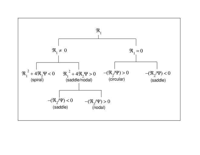
Figure 1: Classification scheme for critical points. For details see section II.5.

The solutions are classified according to their topological behaviour in the neighbourhood of the fixed points. If $\Re_{1}$ is non-zero, the inequality ${\Re_{1}}^{2}<4\Re_{2}\Psi$ indicates that the fixed point is of a spiral type, and if ${\Re_{1}}^{2}>4\Re_{2}\Psi$, the fixed point is of a saddle type for $\Re_{2}>0$ or a nodal type for $\Re_{2}<0$. If $\Re_{1}=0$, there are no nodal points, and the spiral points become of a circular type when $\Re_{2}<0$. The saddle-type fixed points in this case correspond to the condition $\Re_{2}>0$. The classification scheme for the critical points is depicted by the flow chart diagram shown in Fig. 1.

For a particular value of $\left({\cal E},\lambda,\gamma\right)$, Eqs. (26)-(43) can be solved simultaneously to obtain a transonic solution passing through the critical point represented by $\left({\cal E},\lambda,\gamma\right)$. However, one should note that an ‘acceptable’ physical transonic solution must be globally consistent, i.e. it must connect the radial infinity $r{\rightarrow}\infty$ with the black-hole event horizon $r=2r_{g}$. This acceptability constraint further demands that the critical point corresponding to the flow should be of a saddle or a nodal type. This condition is necessary although not sufficient, as we discuss in the following sections. Spiral or centre-type critical points do not admit a globally acceptable solution. For further discussion on the classification of critical points, see, eg. ferrari ; kato and references therein.

II.6 Distinction between critical points and sonic points

Before we proceed, let us discuss one important issue regarding the relation between the critical points and the sonic points in this work. From Eq. (34) one can calculate the Mach number of the flow at the critical point as

$$M_{c}=\sqrt{\left({\frac{2}{\gamma+1}}\right)\frac{{f_{1}}(r_{c},\lambda)}{{{f_{1}}(r_{c},\lambda)}+{{f_{2}}(r_{c},\lambda)}}}\,.$$ (44)

Clearly, $M_{c}$ is generally not equal to one, and for $\gamma\geq 1$, is always less than one. Hence we distinguish a sonic point from a critical point. In the literature on transonic black-hole accretion discs, the concepts of critical and sonic points are often made synonymous by defining an ‘effective’ sound speed leading to the ‘effective’ Mach number (for further details, see, eg. matsumoto ; sandy ). Such definitions were proposed as effects of a specific disc geometry. We, however, prefer to maintain the usual definition of the Mach number for two reasons.

First, in the existing literature on transonic disc accretion, the Mach number at the critical point turns out to be a function of $\gamma$ only, and hence $M_{c}$ remains constant if $\gamma$ is constant. For example, using the Paczyński and Wiita wiita pseudo-Schwarzschild potential to describe the accretion phenomena leads to

$$M_{c}=\sqrt{\frac{2}{\gamma+1}}\,.$$ (45)

However, the quantity $M_{c}$ in Eq. (44) is clearly a function of $r_{c}$, and hence, generally, it takes different values for different $r_{c}$ for multi-transonic accretion, even at a fixed value of $\left({\cal E},\lambda,\gamma\right)$. In the following paragraphs we show that the difference between the radii of the critical point and the sonic point may be quite significant. We define the radial difference as

$${\Delta}r_{c}^{s}=|r_{s}-r_{c}|.$$ (46)

The quantity ${\Delta}r_{c}^{s}$ may be a complicated function of $\left({\cal E},\lambda,\gamma\right)$, the form of which can not be expressed analytically. The radius $r_{s}$ in Eq. (46) is the radius of the sonic point corresponding to the same $\left({\cal E},\lambda,\gamma\right)$ for which the radius of the critical point $r_{c}$ is evaluated. Note, however, that since $r_{s}$ is calculated by integrating the flow from $r_{c}$, ${\Delta}r_{c}^{s}$ is defined only for saddle-type critical points. This is because, as we will see in the subsequent sections, a physically acceptable transonic solution can be constructed only through a saddle-type critical point. One can then show that ${\Delta}r_{c}^{s}$ can be as large as $10^{2}$ $r_{g}$ or even more (for details, see section III.5).

The second and perhaps the more important reason for keeping $r_{c}$ and $r_{s}$ distinct is the following. In addition to studying the dynamics of general relativistic transonic black-hole accretion, we are also interested in studying the analogue Hawking effects for such accretion flow. We need to identify the location of the acoustic horizon as a radial distance at which the Mach equals to one, hence, a sonic point, and not a critical point will be of our particular interest. To this end, we first calculate the critical point for a particular $\left({\cal E},\lambda,\gamma\right)$ following the procedure discussed above, and then we compute the location of the sonic point by integrating the flow equations starting from the critical points. The details of this procedure are provided in the following sections. Furthermore, the definition of the acoustic metric in terms of the sound speed does not seem to be mathematically consistent with the idea of an ‘effective’ sound speed, irrespective of whether one deals with the Newtonian, post Newtonian, or a relativistic description of the accretion disc. Hence, we do not adopt the idea of identifying critical with sonic points. However, for saddle-type critical points, $r_{c}$ and $r_{s}$ should always have one-to-one correspondence, in the sense that every critical point that allows a steady solution to pass through it is accompanied by a sonic point, generally at a different radial distance $r$.

It is worth emphasizing that the distinction between critical and sonic points is a direct manifestation of the non-trivial functional dependence of the disc thickness on the fluid velocity, the sound speed and the radial distance. In the simplest idealized case when the disc thickness is assumed to be constant, one would expect no distinction between critical and sonic points. In this case, as has been demonstrated for a thin disc accretion onto the Kerr black hole abraham , the quantity $\Delta r_{c}^{s}$ vanishes identically for any astrophysically relevant value of $\cal E$, $\lambda$, $\gamma$, and the Kerr black-hole spin parameter $a$.

III Global classification of the $\left[{\cal E},\lambda,\gamma\right]$ space based on the nature of the critical points

III.1 Choice of $\left[{\cal E},\gamma\right]$ and the classification scheme

Next, we give a complete classification scheme for the critical points and the corresponding flow solutions, for the parameter space spanned by all astrophysically relevant values of $\left[{\cal E},\lambda,\gamma\right]$. We first set the appropriate bounds on $\left[{\cal E},{\gamma}\right]$ to model the realistic situations encountered in astrophysics. Since the specific energy ${\cal E}$ includes the rest-mass energy, ${\cal E}=1$ is the lower bound which corresponds to a flow with zero thermal energy at infinity. Hence, the values ${\cal E}<1$, corresponding to the negative energy accretion states, would be allowed if a mechanism for a radiative extraction of the rest-mass energy existed. The possibility of such an extraction would in turn imply viscosity or other dissipative mechanisms in the fluid, the properties which would violate Lorenz invariance. Since Lorenz invariance is a prerequisite for studying the analogue Hawking effects, we concentrate only on non-dissipative flows, and hence, we exclude ${\cal E}<1$. On the other hand, although almost all ${\cal E}>1$ are theoretically allowed, large values of ${\cal E}$ represent flows starting from infinity with very high thermal energy. In particular, ${\cal E}>2$ accretion represents enormously hot flow configurations at very large distance from the black hole, which are not properly conceivable in realistic astrophysical situations. Hence, we set $1{\lower 2.15277pt\hbox{$\;\buildrel<\over{\sim}\;$}}{\cal E}{\lower 2.15277pt\hbox{$\;\buildrel<\over{\sim}\;$}}2$.

The physical lower bound on the polytropic index is $\gamma=1$, which corresponds to isothermal accretion where accreting fluid remains optically thin. Hence, the values $\gamma<1$ are not realistic in accretion astrophysics. On the other hand, $\gamma>2$ is possible only for superdense matter with a very large magnetic field and a direction-dependent anisotropic pressure. The presence of a magnetic field would in turn require solving the general relativistic magneto-hydrodynamic equations, which is beyond the scope of this paper. Thus, we set $1{\lower 2.15277pt\hbox{$\;\buildrel<\over{\sim}\;$}}\gamma{\lower 2.15277pt\hbox{$\;\buildrel<\over{\sim}\;$}}2$. However, astrophysically preferred values of $\gamma$ for realistic black-hole accretion range from $4/3$ (ultra-relativistic) to $5/3$ (purely non-relativistic flow) frank . Hence, we mainly focus on the parameter range

$$\left[1{\lower 2.15277pt\hbox{$\;\buildrel<\over{\sim}\;$}}{\cal E}{\lower 2.15277pt\hbox{$\;\buildrel<\over{\sim}\;$}}2,~{}\frac{4}{3}{\leq}\gamma{\leq}\frac{5}{3}\right].$$ (47)

Figure 2 shows a complete classification scheme for the critical point parameter space together with some representative flow topologies. The figure has been drawn for the fluid with $\gamma=4/3$, but a similar figure may be produced for any other value of astrophysically relevant $\gamma$. The central plot of Fig. 2 depicts the classification of $\left[{\cal E},\lambda\right]$ according to the number and nature of the critical points in the flow. The side panels show the representative topologies for all distinct critical point zones drawn in the central plot. The panel marked by, say, W shows a representative topology for the particular $\left({\cal E},\lambda\right)$ chosen from the region marked by W in the central plot. A thick black cross with a white square at its centre in the W zone indicates the point in the parameter space $\left({\cal E},\lambda\right)$ for which the panel topology W is drawn. The horizontal axis in the panel figures represents the radial distance in units of $r_{g}$ on the logarithmic scale, whereas the vertical axis represents the flow Mach number. The parameters ${\cal E}$ and $\lambda$ for which a particular topology is drawn are written at the top right corner of the corresponding panel figure.

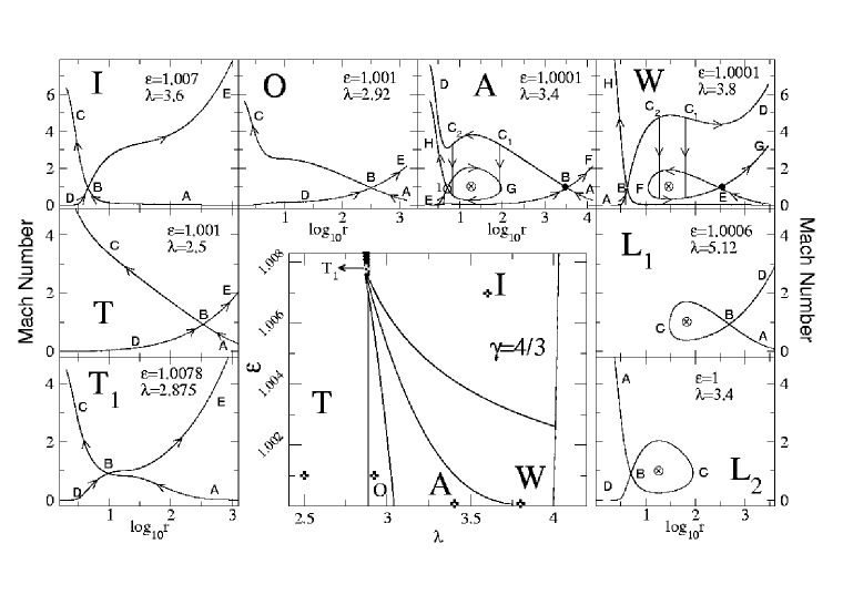
Figure 2: Parameter space division for general relativistic accretion and wind. The side panels show the representative topologies for all distinct critical point zones drawn in the central plot. The bold capitals that mark the side panels correspond to those that mark the regions of the parameter space in the central plot. The points in the parameter space for which the side panels are drawn are marked in the central plot by a thick black cross with a white square at its centre. The inward oriented curves marked by arrow heads indicate accretion, while those oriented outwards indicate wind.

III.2 Mono-transonic solutions with one critical point

The wedge shaped regions marked by O and I in Fig. 2 represent the values of $\left[{\cal E},\lambda\right]$ for which there exists only one critical point, and hence only one sonic point. The accretion is mono-transonic and the critical points are of a saddle type. In the region marked by I, the critical points are called inner critical points since these points are quite close to the event horizon, approximately in the range $2<r_{c}^{\rm inner}{\leq}10$. In the region marked by O, the critical points are called ‘outer critical points’, because these points are located considerably far away from the black hole. Depending on the value of $\left({\cal E},\lambda,\gamma\right)$, an outer critical point may be as far as $10^{4}r_{g}$, or more. The corresponding flow topologies are shown in the panel diagram marked by I and O.

To describe the procedure for obtaining the panel plots, first consider the topology I. Using the value of $\left({\cal E},\lambda,\gamma\right)$ marked in the figure, we first solve Eq. (35) to obtain the corresponding critical point $r_{c}=4.535$ marked in the figure by B at the intersection of the accretion branch ABC and the wind branch DBE. We then calculate the critical value of the advective velocity gradient at $r_{c}$ from Eq. (39)-(43). By integrating (30) and (32) from the critical point B, using the fourth-order Runge-Kutta method, we then calculate the local advective velocity, the polytropic sound speed, the Mach number, the fluid density, the disc height, the bulk temperature of the flow, and any other relevant dynamical and thermodynamic quantity characterizing the flow. In this way we obtain the accretion branch ABC by employing the above mentioned procedure.

Each solution represented in the panel plots in Fig. 2 is two-fold degenerate owing to the $\pm u$ degeneracy which reflects the physical accretion/wind degeneracy. We have, however, removed the degeneracy by orienting the curves, and thus each line represents either the wind or accretion. We have arbitrarily assigned the $+$ sign solution in Eq. (39) to the accretion and the $-$ sign solution in Eq. (39) to the ‘wind’ branch DBE. This wind branch is just a mathematical counterpart of the accretion solution (velocity reversal symmetry of accretion), owing to the presence of the quadratic term of the dynamical velocity in the equation governing the energy momentum conservation.

The term ‘wind solution’ has a historical origin. The solar wind solution first introduced by Parker parker has the same topology profile as that of the wind solution obtained in classical Bondi accretion bondi . Hence the name ‘wind solution’ has been adopted in a more general sense. The wind solution thus represents a hypothetical process, in which, instead of starting from infinity and heading towards the black hole, the flow generated near the black-hole event horizon would fly away from the black hole towards infinity. The topology of such a process is represented by the wind solution DBE.

The above procedure for obtaining the flow topology is also applied to draw the mono-transonic accretion/wind branch through the outer sonic point, i.e. the topology marked by O with $r_{c}^{\bf outer}=318.63$. In fact, the same procedure may be used to draw real physical transonic accretion/wind solutions passing through any acceptable saddle-type critical point. Note, however, that AB in the topology I or O, is not the complete subsonic branch, because B is a critical point and not a sonic point. Using the procedure described above we have to integrate the flow from B to the sonic point where the Mach number equals one. The sonic point is basically equivalent to the acoustic horizon at which the analogue Hawking radiation is emitted. We discuss this issue in detail in sections V and VI. Note that the regions I or O in the central plot do not include the ‘zero energy’ accretion, i.e. a flow parameterized by ${\cal E}=1$, although from the diagram it may so appear. Zero energy mono-transonic accretion does not admit a steady solution passing through the inner or the outer critical point. Note also that the parameter space region I extends up to ${\cal E}=2$ along the horizontal axis, which is not shown in the figure for convenience.

III.3 Mono-transonic solutions with two critical points

The region marked by T in the central plot, including the region marked by ${\bf T}_{1}$ with ${\left[{\cal E},\lambda\right]}_{\bf T_{1}}~{}{\subseteq}~{}{\left[{\cal E},\lambda\right]}_{\bf T}$, represents $\left[{\cal E},\lambda\right]$ for which two critical points exist. We call these two critical points $r_{c}^{1}$ and $r_{c}^{2}$, with $r_{c}^{1}<r_{c}^{2}$. The T region is extended along the horizontal axis to the left up to $\lambda=0$, and along the vertical axis up to ${\cal E}=2$. A small patch of $\left[{\cal E},\lambda\right]|_{\bf T}$ not shown in the figure exists in the range $\left[1.0002{\leq}{\cal E}{\leq}1.0014,~{}5.18{\leq}\lambda{\leq}5.28\right]$. Except this small patch, almost the whole region in the $\left[{\cal E},\lambda\right]$ space beyond the nearly vertical line passing through $\lambda=4$ generally does not admit any real solution for $r_{c}$. The critical points obtained in the region $\left[{\cal E},\lambda\right]_{\bf T}$ can be further classified roughly into three regions for ${\cal E}>1$.

The first subset $\left[{\cal E},\lambda\right]_{\bf T_{1}}$ is depicted in the central plot as a dark triangular zone. For this subset, both sets of critical points $r_{c}^{1}$ and $r_{c}^{2}$ lie within the radial distance of 10$r_{g}$, with $3.1{\leq}r_{c}^{1}{\leq}3.1014$ and $8.6{\leq}r_{c}^{2}{\leq}10$. We have found that $r_{c}^{1}$ is not associated with any steady solution passing through it, whereas there exists a complete mono-transonic accretion/wind solution passing through $r_{c}^{2}$ . However, an accretion solution belonging to this class is topologically not very different from any mono-transonic solution obtained for $\left({\cal E},\lambda\right){\in}{\left[{\cal E},\lambda\right]}_{\bf I}$ or $\left({\cal E},\lambda\right){\in}{\left[{\cal E},\lambda\right]}_{\bf O}$. One such solution is shown in the panel figure marked by T₁. The critical point B for such solution is located at $r_{c}=9.75$. By ‘complete’ solution, we refer to a solution that extends from $r=2$ to $r{\rightarrow}{\infty}$.

The second subset of $\left[{\cal E},\lambda\right]_{\bf T}$ corresponds to the cases where $r_{c}^{1}$ ranges from 2 to 10, while $r_{c}^{2}$ is substantially larger. Similarly, in this region we do not find any steady solution passing through $r_{c}^{1}$ and we find a complete steady, transonic solution passing through $r_{c}^{2}$. Such a solution is shown in the side panel marked by T with the critical point at about $r_{c}=335$.

The third subset of $\left[{\cal E},\lambda\right]_{\bf T}$, as mentioned earlier, is $\left[1.0002{\leq}{\cal E}{\leq}1.0014,~{}5.18{\leq}\lambda{\leq}5.28\right]$. Here $r_{c}^{1}$ ranges approximately from 60 to 115 and $r_{c}^{2}$ approximately from 150 to 3500. Again, steady solutions passing through $r_{c}^{1}$ do not exist. However, the solutions passing through $r_{c}^{2}$ are steady, but not complete, because those solutions form an outbound loop round the corresponding $r_{c}^{1}$ enclosed in the loop. One such representative solution is shown in the side panel L₁. The critical point $r_{c}^{2}=486.79$ is marked by B and the corresponding $r_{c}^{1}=64.08$ is marked by a crossed circle $\otimes$.

In the above discussion, we have concentrated on the solutions for which ${\cal E}>1$. In Fig. 3 we plot $r_{c}$ as a function of $\lambda$ for the zero energy accretion, i.e. the accretion with ${\cal E}=1$. The solid line AB represents $r_{c}^{1}$, whereas the dashed line represents $r_{c}^{2}$. We find no steady solutions passing through $r_{c}^{2}$, whereas there exists a solution passing through $r_{c}^{1}$ which is smooth but incomplete as it forms an inward bound loop round $r_{c}^{2}$ enclosed in the loop. In the panel figure marked by L₂, we plot one representative of such topology. The critical point $r_{c}^{1}=5.1$ is marked by B and the corresponding $r_{c}^{2}=18.19$ is marked by a crossed circle $\otimes$. The curve ABCD represents the incomplete accretion (ABC)/wind (DBC) solution. Interestingly, this structure is topologically similar to the inward bound loop representing the incomplete accretion/wind branch of a multi-transonic accretion which we discuss in the next paragraph.

Note here that the accretion with two critical points can practically be considered as an example of mono-transonic accretion. Since one of the two critical points (either $r_{c}^{1}$ or $r_{c}^{2}$) does not belong to any steady flow through it, only the other critical point admits a steady flow to pass through it, and hence there will be only one sonic point associated with it.

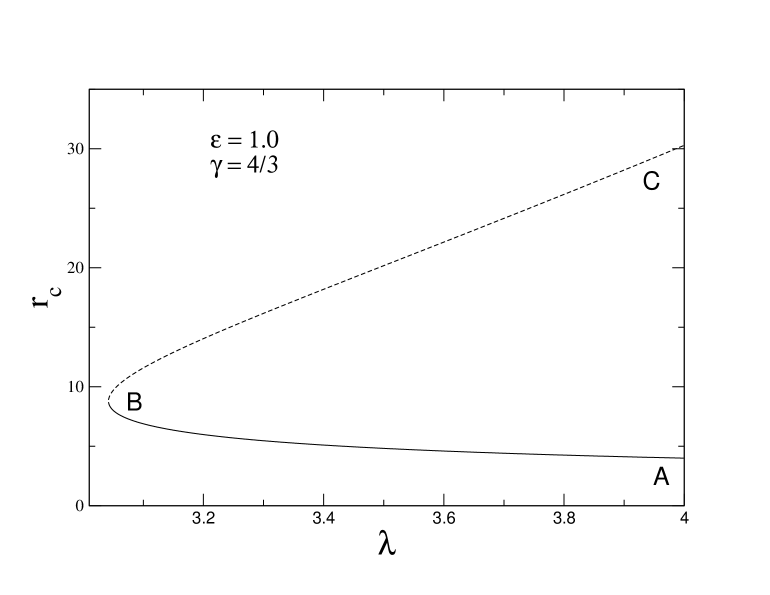
Figure 3: Zero energy (${\cal E}=1$) accretion flow with two critical points. The solid line AB represents the set of inner critical points. The flow passing through an inner critical point has a closed loop topology as shown in the side panel L₂ of Fig. 2. The dashed line represents the set of outer critical points. There is no steady solution passing through an outer critical point.

III.4 Multi-transonic accretion and wind

The wedge shaped region marked by A in the central figure corresponds to the multi-transonic accretion. For any $\left({\cal E},\lambda\right){\in}{\left[{\cal E},\lambda\right]}_{\bf A}$, the flow has three critical points The corresponding flow topology is shown in the panel figure marked by A. The line ABC₁C₂D represents a complete transonic solution passing through the saddle-type outer critical point B at $r_{c}=3310.88$. The solid circle $\bullet$ marks the outer sonic point at $r_{s}^{\rm outer}=2930.47$ where the flow Mach number is equal to one. The corresponding wind solution is shown by the line EBF. The crossed circle $\otimes$ marks the location of the centre-type middle critical point at $r_{c}^{\bf middle}=18.32$, through which a steady solution cannot be constructed. The line EIGH represents the incomplete accretion (GIH)/wind (EIG) solution passing through the saddle type inner critical point I at $r_{c}=5.097$. The corresponding inner sonic point $r_{s}^{\rm inner}$ (not shown in the figure) is located at $r_{s}=4.903$. Clearly, this loop structure is very similar to the zero energy accretion topology shown in the panel plot L₂.

The set $\left[{\cal E},\lambda\right]_{\bf A}$ (or more generally $\left[{\cal E},\lambda,\gamma\right]_{\bf A}$) thus produces doubly degenerate accretion/wind solutions. Such two fold degeneracy may be removed by the entropy considerations since the entropy rates ${\dot{S}}$($r_{c}^{\rm inner}$) and ${\dot{S}}$($r_{c}^{\rm outer}$) are generally not equal. For any $\left({\cal E},\lambda\right){\in}{\left[{\cal E},\lambda\right]}({\bf A})$, we find that the entropy rate ${\dot{S}}$ evaluated for the complete accretion solution passing through the outer critical point is less than that of the rate evaluated for the incomplete accretion/wind solution passing through the inner critical point. Since the quantity ${\dot{S}}$ is a measure of the specific entropy density of the flow, the solution passing through $r_{c}^{\rm outer}$ will naturally tend to make a transition to its higher entropy counterpart, i.e. the incomplete accretion solution passing through $r_{c}^{\rm inner}$. Hence, if there existed a mechanism for the solution ABC₁C₂D to increase its entropy accretion rate by an amount

$${\Delta}{\dot{S}}={\dot{S}}(r_{c}^{\rm inner})-{\dot{S}}(r_{c}^{\rm outer}),$$ (48)

there would be a transition to the incomplete solution GIH. Such a transition would take place at a radial distance somewhere between the radius of the inner sonic point and the radius of the accretion/wind turning point ($r=94.9$ for this case) marked by G. In this way one would obtain a combined accretion solution connecting $r{\rightarrow}{\infty}$ with $r=2$ which includes a part of the accretion solution passing through the inner critical, and hence the inner sonic point. One finds that for some specific values of $\left[{\cal E},\lambda,\gamma\right]{\subseteq}{\left[{\cal E},\lambda,\gamma\right]}_{\bf A}$, a standing Rankine-Hugoniot shock may accomplish this task. A supersonic accretion through the outer sonic point $r_{s}^{\rm outer}$ can generate entropy through such a shock formation and can join the flow passing through $r_{s}^{\rm inner}$. Although two shock locations, indicated by the vertical lines through C₁ and C₂ with a downward arrow, are found, only one of the two shocks is stable. We discuss the details of such a shock formation in section IV.

The wedge shaped region marked by W in the central figure represents the $\left[{\cal E},\lambda\right]$ zone for which three critical points, the inner, the middle and the outer are also found. However, in contrast to $\left[{\cal E},\lambda\right]_{\bf A}$, the set $\left[{\cal E},\lambda\right]_{\bf W}$ yields solutions for which ${\dot{S}}(r_{c}^{\rm inner})$ is less than ${\dot{S}}(r_{c}^{\rm outer})$. Besides, the topological flow profile of these solutions is different. One such solution topology is presented in the panel plot marked by W. Here the loop-like structure is formed through the outer critical point. Note a similarity with the topology L₁. This topology is interpreted in the following way. The flow HB passing through the inner critical point B at $r_{c}=4.25$ is the complete mono-transonic accretion flow, and ABC₂C₁D is its corresponding wind solution. The solution EFG passing through the outer critical point E at $r_{c}^{\rm outer}=301.53$, with the corresponding outer sonic point marked by a solid circle $\bullet$ located at $r_{s}^{\rm outer}=343.312$ represents the incomplete accretion (EF)/wind (FG) solution. The initially subsonic wind solution passing through $r_{c}^{\rm inner}$ encounters the outer sonic point at $r_{s}^{\rm inner}=(4.31$, and becomes supersonic. However, as ${\dot{S}}_{\rm ABC_{2}C_{1}D}$ turns out to be less than ${\dot{S}}_{\rm FEG}$, the solution branch ABC₂C₁D can make a shock transition to join its counter solution FEG and thereby increase the entropy accretion rate by the amount ${\Delta}{\dot{S}}={\dot{S}}_{\rm ABC_{2}C_{1}D}-{\dot{S}}_{\rm FEG}$. Here, two theoretical shock locations are obtained, out of which only one is stable. Hence the set $\left[{\cal E},\lambda,\gamma\right]_{\bf W}$ corresponds to mono-transonic accretion solutions with multi-transonic wind solutions with a shock.

Besides $\gamma=4/3$, for which Fig. 2 has been drawn, we could perform a similar classification for any astrophysically relevant value of $\gamma$ as well. Some characteristic features of $\left[{\cal E},\lambda\right]$ would be changed as we vary $\gamma$. For example, if ${\cal E}_{\rm max}$ is the maximum value of the energy and if $\lambda_{\rm max}$ and $\lambda_{\rm min}$ are the maximum and the minimum values of the angular momentum, respectively, for $\left[{\cal E},\lambda\right]_{\bf A}$ for a fixed value of $\gamma$, then $\left[{\cal E}_{\rm max},\lambda_{\rm max},\lambda_{\rm min}\right]$ anti-correlates with $\gamma$. Hence, as the flow makes a transition from its ultra-relativistic to its purely non-relativistic limit, the area representing $\left[{\cal E},\lambda\right]_{\bf A}$ decreases.

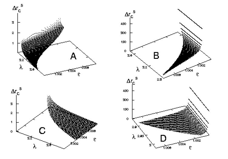
Figure 4: The difference $\Delta{r_{c}^{s}}$ between of the sonic points radius $r_{s}$ and the critical point radius $r_{c}$ as a function of the specific energy ${\cal E}$ and the specific angular momentum $\lambda$. The plots represent a mono-transonic flow passing through the inner critical point (plot A) and the outer critical point (plot B); a multi-transonic accretion passing through the inner critical point (plot C) and the outer critical point (plot D).

III.5 Dependence of $\Delta{r_{c}^{s}}$ on $\left[{\cal E},\lambda,\gamma\right]$

Here, we study the dependence of the radial difference between the critical points and the sonic points on fundamental accretion parameters. In Fig. 4, the difference ${\Delta}r_{c}^{s}$ defined by Eq. (46) is plotted as a function of the specific flow energy ${\cal E}$ and the specific angular momentum $\lambda$ for a mono-transonic flow passing through the inner critical point (plot A) and the outer critical point (plot B), and for a multi-transonic accretion flow passing through the inner critical point (plot C) and the outer critical point (plot D). Obviously, the radial difference between the sonic point and the critical point may be quite significant, especially for the accretion/wind flow passing through the outer critical and sonic points.The quantity ${\Delta}r_{c}^{s}$ anti-correlates with $\lambda$ for a general flow, whereas it correlates with ${\cal E}$ for a flow passing through the inner critical point and anti-correlates with ${\cal E}$ for a flow passing through the outer critical point.

III.6 Onset of chaotic behaviour in multi-transonic flow

In the central part of figure 2 the boundary between the O and the A zone, and between the W and the I zone, provides interesting information about the possibility of the onset of chaotic behaviour of the multi-transonic accretion flow. According to the theory of dynamical systems (see, e.g. jordan ), if a small change of the control parameters leads to profound effects on the outcome of the whole system, the system may then be considered to exhibit chaotic behaviour. Along the boundary between O and A, an extremely small change of ${\lambda}$ or ${\cal E}$ (or $\gamma$ if there were a transition across the bounding surface between $\left[{\cal E},\lambda,\gamma\right]_{\bf O}$ and $\left[{\cal E},\lambda,\gamma\right]_{\bf A}$) would lead to a sharp transition from a mono-transonic to a multi-transonic flow (and vice versa). A similar situation arises for the $\left[{\cal E},\lambda\right]_{\bf W}{\longleftrightarrow}\left[{\cal E},\lambda\right]_{\bf I}$ transition.

The above phenomenon is an example of the bifurcation of critical points due to a slight change in the control parameters. It is possible to study the onset of chaotic behaviour even for a stationary system. Bray and Moore bray , for example, studied the spin-glass phase in terms of a $T=0$ fixed point, and established a criteria for the onset of chaos in such a system by proposing an effective Lyapunov exponent. In a similar way we propose an effective Lyapunov exponent for a transonic flow solution. Let $u_{1}(r)$ and $u_{2}(r)$ be the values of the advective velocity at any radial distance $r$ for two transonic solutions characterized by very close values of the angular momentum $\lambda_{1}$ and $\lambda_{2}$ respectively , i.e. $\left(\lambda_{1}-\lambda_{2}\right){\longrightarrow}0$, with ${\cal E}$ and $\gamma$ kept fixed. Let $u_{1}(r+R)$ and $u_{2}(r+R)$ be the corresponding velocities for the above-mentioned transonic flow solutions at the radial distance $r+R$. We then define the effective Lyapunov exponent $L_{eff}$, so that the following condition holds:

$$\frac{u_{1}(r+R)-u_{2}(r+R)}{u_{1}(r)-u_{2}(r)}\sim e^{L_{eff}R}.$$ (49)

The quantity $L_{eff}$ can also be calculated by varying ${\cal E}$ instead of $\lambda$. Next, one can show that the system will be sensitive to the initial boundary conditions if $L_{eff}>0$. The preliminary calculation naku indeed indicates such values of $L_{eff}>0$ for a transition from mono- to multi-transonic flow, and vice versa. Hence, transonic flow solutions exhibit chaotic behaviour. Investigation of chaos in black-hole accretion discs may shed a new light on the explanation of the variability mechanism of active galactic nuclei (for details about AGN variability, see, e.g. milwit ). However, the details of the calculation are beyond the scope of this paper and will be presented elsewhere.

IV Shock formation in relativistic accretion

IV.1 A general overview

Perturbations of various kinds may produce discontinuities in an astrophysical fluid flow. By discontinuity at a surface in a fluid flow we understand any discontinuous change of a dynamical or a thermodynamic quantity across the surface. The corresponding surface is called a surface of discontinuity. Certain boundary conditions must be satisfied across such surfaces and according to these conditions, surfaces of discontinuities are classified into various categories. The most important such discontinuities are shock waves or shocks. In an adiabatic flow of the Newtonian fluid, the shocks obey the following conditions landau :

$$\left[\left[{\rho}u\right]\right]=0,~{}\left[\left[p+{\rho}u^{2}\right]\right]=0,~{}\left[\left[\frac{u^{2}}{2}+h\right]\right]=0,$$ (50)

where $[[f]]$ denotes the discontinuity of $f$ across the surface of discontinuity, i.e.

$$\left[\left[f\right]\right]=f_{2}-f_{1},$$ (51)

with $f_{2}$ and $f_{1}$ being the boundary values of the quantity $f$ on the two sides of the surface. Such shock waves are quite often generated in various kinds of supersonic astrophysical flows having intrinsic angular momentum, resulting in a flow which becomes subsonic. This is because the repulsive centrifugal potential barrier experienced by such flows is sufficiently strong to brake the infalling motion and a stationary solution could be introduced only through a shock. Rotating, transonic astrophysical fluid flows are thus believed to be ‘prone’ to the shock formation phenomena.

One also expects that a shock formation in black-hole accretion discs might be a general phenomenon because shock waves in rotating astrophysical flows potentially provide an important and efficient mechanism for conversion of a significant amount of the gravitational energy into radiation by randomizing the directed infall motion of the accreting fluid. Hence, the shocks play an important role in governing the overall dynamical and radiative processes taking place in astrophysical fluids and plasma accreting onto black holes. The study of steady, standing, stationary shock waves produced in black hole accretion has acquired a very important status in recent years. For details and for an exhaustive list of references see, e.g. apj1 .

Generally, the issue of the formation of steady, standing shock waves in black-hole accretion discs is addressed in two different ways. First, one can study the formation of Rankine-Hugoniot shock waves in a polytropic flow. Radiative cooling in this type of shock is quite inefficient. No energy is dissipated at the shock and the total specific energy of the accreting material is a shock-conserved quantity. Entropy is generated at the shock and the post-shock flow possesses a higher entropy accretion rate than its pre-shock counterpart. The flow changes its temperature permanently at the shock. Higher post-shock temperature puffs up the post-shock flow and a quasi-spherical, quasi-toroidal centrifugal pressure supported region is formed in the inner region of the accretion disc apj1 .

Another class of the shock studies concentrates on the shock formation in isothermal black-hole accretion discs. The characteristic features of such shocks are quite different from the non-dissipative shocks discussed above. In isothermal shocks, the accretion flow dissipates a part of its energy and entropy at the shock surface to keep the post-shock temperature equal to its pre-shock value. This maintains the vertical thickness of the flow exactly the same just before and just after the shock is formed. Simultaneous jumps in energy and entropy join the pre-shock supersonic flow to its post-shock subsonic counterpart. For detailed discussion and references see, e.g. apj2 ; tsuruta .

In this work, the basic equations governing the flow are the energy and baryon number conservation equations which contain no dissipative terms and the flow is assumed to be inviscid. Hence, the shock which may be produced in this way can only be of Rankine-Hugoniot type which conserves energy. The shock thickness must be very small in this case, otherwise non-dissipative flows may radiate energy through the upper and the lower boundaries because of the presence of strong temperature gradient in between the inner and outer boundaries of the shock thickness. In the presence of a shock the flow may experience the following profile. A subsonic flow starting from infinity first becomes supersonic after crossing the outer sonic point and somewhere in between the outer sonic point and the inner sonic point the shock transition takes place and forces the solution to jump onto the corresponding subsonic branch. The hot and dense post-shock subsonic flow produced in this way becomes supersonic again after crossing the inner sonic point and ultimately dives supersonically into the black hole. A flow heading towards a neutron star can have the liberty of undergoing another shock transition after it crosses the inner sonic point , because the hard surface boundary condition of a neutron star by no means prevents the flow from hitting the star surface subsonically.

IV.2 The relativistic Rankine-Hugoniot conditions

For the complete general relativistic accretion flow discussed in this work, the energy momentum tensor ${T}^{{\mu}{\nu}}$, the four-velocity $v_{\mu}$, and the speed of sound $c_{s}$ may have discontinuities at a hypersurface $\Sigma$ with its normal $\eta_{\mu}$. Using the energy momentum conservation and the continuity equation, one has

$$\left[\left[{\rho}v^{\mu}\right]\right]{\eta}_{\mu}=0,\left[\left[{T}^{\mu\nu}\right]\right]{\eta}_{\nu}=0.$$ (52)

For a perfect fluid, one can thus formulate the relativistic Rankine-Hugoniot conditions as

$$\left[\left[{\rho}u\Gamma_{u}\right]\right]=0,$$ (53)

$$\left[\left[{T}_{t\mu}{\eta}^{\mu}\right]\right]=\left[\left[(p+\epsilon)v_{t}u\Gamma_{u}\right]\right]=0,$$ (54)

$$\left[\left[{T}_{\mu\nu}{\eta}^{\mu}{\eta}^{\nu}\right]\right]=\left[\left[(p+\epsilon)u^{2}\Gamma_{u}^{2}+p\right]\right]=0,$$ (55)

where $\Gamma_{u}=1/\sqrt{1-u^{2}}$ is the Lorentz factor. The first two conditions (53) and (54) are trivially satisfied owing to the constancy of the specific energy and mass accretion rate. The constancy of mass accretion yields

$$\left[\left[K^{-\frac{1}{\gamma-1}}\left(\frac{\gamma-1}{\gamma}\right)^{\frac{1}{\gamma-1}}\left(\frac{c_{s}^{2}}{\gamma-1-c_{s}^{2}}\right)^{\frac{1}{\gamma-1}}uc_{s}\sqrt{\frac{r^{3}-{\lambda^{2}}\left(r-2\right)}{\gamma-\left(1+c_{s}^{2}\right)}}\right]\right]=0.$$ (56)

The third Rankine-Hugoniot condition (55) may now be written as

$$\left[\left[K^{-\frac{1}{\gamma-1}}\left(\frac{\gamma-1}{\gamma}\right)^{\frac{\gamma}{\gamma-1}}\left(\frac{c_{s}^{2}}{\gamma-1-c_{s}^{2}}\right)^{\frac{\gamma}{\gamma-1}}\left\{\frac{u^{2}\left(\gamma-c_{s}^{2}\right)+c_{s}^{2}}{c_{s}^{2}\left(1-u^{2}\right)}\right\}\right]\right]=0.$$ (57)

Simultaneous solution of Eqs. (56) and (57) yields the ‘shock invariant’ quantity

$${\cal S}_{h}=\frac{u^{2}\left(\gamma-c_{s}^{2}\right)+c_{s}^{2}}{c_{s}{u}\left(1-u^{2}\right)\sqrt{\gamma-1-c_{s}^{2}}}$$ (58)

which changes continuously across the shock surface. We also define the shock strength ${\cal S}_{i}$ and the entropy enhancement $\Theta$ as the ratio of the pre-shock to post-shock Mach numbers (${\cal S}_{i}=M_{-}/M_{+}$), and as the ratio of the post-shock to pre-shock entropy accretion rates ($\Theta={\dot{S}}_{+}/{\dot{S}}_{-}$) of the flow, respectively.

IV.3 Shock locations in multi-transonic accretion and wind

The shock location in multi-transonic accretion is found in the following way. Consider the multi-transonic flow topology A in Fig. 2. Integrating along BC₁C₂D, we calculate the shock invariant ${\cal S}_{h}$ in addition to $u$, $c_{s}$ and $M$. We also calculate ${\cal S}_{h}$ while integrating the sector HIG, starting from the inner sonic point up to the point of inflexion G. We then determine the radial distance $r_{sh}$, where the numerical values of ${\cal S}_{h}$, obtained by integrating the two different sectors described above, are equal. Generally, for any value of $\left({\cal E},\lambda,\gamma\right)$ allowing shock formation, one finds two shock locations marked by C₁ (the ‘outer’ shock – between the outer and the middle sonic points) and C₂ (the ‘inner’ shock – between the inner and the middle sonic points) in the figure. According to a standard local stability analysis kafatos , for a multi-transonic accretion one can show that only the shock formed between the middle and the outer sonic point is stable. Hence, in the multi-transonic accretion with the topology A, the shock at C₁ is stable and that at C₂ is unstable. Hereafter, whenever we mention the shock location, we refer to the stable shock location only.

The topology W in Fig. 2 shows the shock formation in the multi-transonic wind. Here the numerical values of ${\cal S}_{h}$ along the wind solution passing through the inner sonic point (line BC₂C₁D) are compared with the numerical values of ${\cal S}_{h}$ along the wind solution passing through the outer sonic point, and the shock locations $C_{1}$ and $C_{2}$ for the wind are found accordingly.

IV.4 Geometry of the accretion with shock and generation of accretion-powered outflow

As a consequence of the shock formation in an accretion, the post-shock flow temperature will also increase abruptly. In Fig. 5, we plot the temperature of the combined accretion flow BC₁IH of the topology A presented in Fig. 2. The segment AB corresponds to the pre-shock flow (BC₁ in the topology A of Fig. 2), while the segment CD corresponds to the post-shock flow. The vertical segment BC is a discontinuous increase of the flow temperature due to the shock formation. The length of BC, which measures the post- to pre-shock temperature ratio $T_{+}/T_{-}$ is, in general, a sensitive function of $\left[{\cal E},\lambda,\gamma\right]$.

In Fig. 6, we present the disc structure obtained by solving Eq. (29) for the combined accretion flow BC₁IH with the topology A in Fig. 2. The point BH represents the black-hole event horizon. The pre- and post-shock regions of the disc are clearly distinguished in the figure and show that the post-shock disc puffs up significantly. It is clear from Fig. 5 that the bulk flow temperature will be increased in the post-shock region. Such an increased disc temperature may lead to a disc evaporation resulting in the formation of an optically thick halo. Besides, a strong temperature enhancement may lead to the formation of thermally driven outflows. The generation of centrifugally driven and thermally driven outflows from black-hole accretion discs has been discussed in the post-Newtonian framework dc99 ; santosh . The post-Newtonian approach may be extended to general relativity using the formalism presented here.

Owing to the very high radial component of the infall velocity of accreting material close to the black hole, the viscous time scale is much larger than the infall time scale. Hence, in the vicinity of the black hole, a rotating inflow entering the black hole will have an almost constant specific angular momentum for any moderate viscous stress. This angular momentum yields a very strong centrifugal force which increases much faster than the gravitational force. These two forces become comparable in size at some specific radial distance. At that point the matter starts piling up and produces a boundary layer supported by the centrifugal pressure, which may break the inflow to produce the shock. This actually happens not quite at the point where the gravitational and centrifugal forces become equal but slightly farther out owing to the thermal pressure. Still closer to the black hole, gravity inevitably wins and matter enters the horizon supersonically after passing through a sonic point. The formation of such a layer may be attributed to the shock formation in accreting fluid. The post-shock flow becomes hotter and denser and, for all practical purposes, behaves as the stellar atmosphere as far as the formation of outflows is concerned. A part of the hot and dense shock-compressed in-flowing material is then ‘squirted’ as an outflow from the post-shock region. Subsonic outflows originating from the puffed up hotter post-shock accretion disc (as shown in the figure) pass through the outflow sonic points and reach large distances as in a wind solution.

The generation of such shock-driven outflows is a reasonable assumption. A calculation describing the change of linear momentum of the accreting material in the direction perpendicular to the plane of the disc is beyond the scope of the disc model used in this work because the explicit variation of dynamical variables along the Z axis (axis perpendicular to the equatorial plane of the disc) cannot be treated analytically. The enormous post-shock thermal pressure is capable of providing a substantial amount of ‘hard push’ to the accreting material against the gravitational attraction of the black hole. This ‘thermal kick’ plays an important role in re-distributing the linear momentum of the inflow and generates a non-zero component along the Z direction. In other words, the thermal pressure at the post-shock region, being anisotropic in nature, may deflect a part of the inflow perpendicular to the equatorial plane of the disc. Recent work shows that monica such shock-outflow model can be applied to successfully investigate the origin and dynamics of the strong X-ray flares emaneting out from our galactic centre.

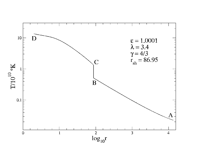
Figure 5: Bulk temperature profile of a multi-transonic accretion flow for $\left({\cal E},\lambda,\gamma\right)$ shown with a shock at $r_{sh}$ . The vertical axis is the flow temperature in units of 10¹⁰ K and the horizontal axis is the radial distance in logarithmic scale. The sector AB represents the pre-shock flow, the sector CD the post-shock flow, and the segment BC is the discontinuous increase of the flow temperature due to the shock formation.

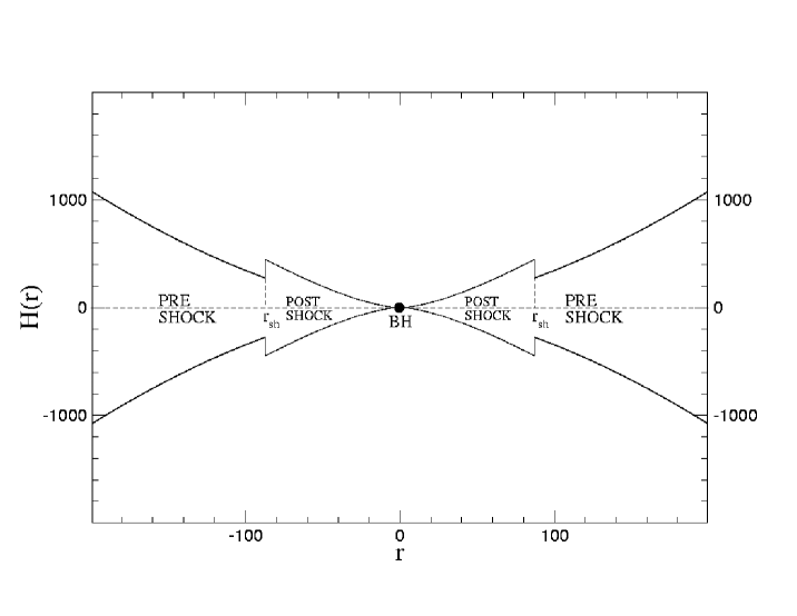
Figure 6: Disc structure of a multi-transonic accretion flow with a shock at $r_{sh}$. The disc height (vertical axis) is plotted as a function of the radial distance (horizontal axis). The point BH represents the black-hole event horizon.

IV.5 Dependence of the shock location on $\left[{\cal E},\lambda,\gamma\right]$

We find that the shock location correlates with $\lambda$. This is obvious because the higher the flow angular momentum, the greater the rotational energy content of the flow. As a consequence, the strength of the centrifugal barrier which is responsible to break the incoming flow by forming a shock will be higher and the location of such a barrier will be farther away from the event horizon. However, the shock location anti-correlates with ${\cal E}$ and $\gamma$. This means that for the same ${\cal E}$ and $\lambda$, in the purely non-relativistic flow the shock will form closer to the black hole compared with the ultra-relativistic flow. Besides, we find that the shock strength ${\cal S}_{i}$ anti-correlates with the shock location $r_{sh}$, which indicates that the closer to the black hole the shock forms , the higher the strength ${\cal S}_{i}$ and the entropy enhancement ratio $\Theta$ are. The ultra-relativistic flows are supposed to produce the strongest shocks. The reason behind this is also easy to understand. The closer to the black hole the shock forms, the higher the available gravitational potential energy must be released, and the radial advective velocity required to have a more vigorous shock jump will be larger. Besides we note that as the flow gradually approaches its purely non-relativistic limit, the shock may form for lower and lower angular momentum, which indicates that for purely non-relativistic accretion, the shock formation may take place even for a quasi-spherical flow. However, it is important to mention that a shock formation will be allowed not for every $\left({\cal E},\lambda\right){\in}{\left[{\cal E},\lambda\right]}({\bf A})$ (or $\left({\cal E},\lambda\right){\in}{\left[{\cal E},\lambda\right]}({\bf W})$) . Equation (58) will be satisfied only for a specific subset of $\left[{\cal E},\lambda\right]({\bf A})$ (or $\left[{\cal E},\lambda\right]({\bf W})$), for which a steady, standing shock solution will be found.

V Acoustic geometry, acoustic horizons, and phonon quantization

Before delving into the calculation of $T_{AH}$ for various kinds of sonic horizon generated in the accretion disc, we would first like to discuss the relevant features of the acoustic geometry.

V.1 Nonrelativistic acoustic geometry

Let $\psi$ denote the velocity potential describing the fluid flow in Newtonian space-time, i.e. let ${\vec{u}}=-{\nabla}\psi$, where ${\vec{u}}$ is the velocity vector describing the dynamics of a Newtonian fluid. The specific enthalpy $h$ of a barotropic Newtonian fluid satsfies ${\nabla}h=(1/{\rho}){\nabla}p$, where $\rho$ and $p$ are the density and the pressure of the fluid. One then writes the Euler equation as

$$-{\partial}_{t}{\psi}+h+\frac{1}{2}\left({\nabla}{\psi}\right)^{2}+\Phi=0,$$ (59)

where $\Phi$ represents the potential associated with any external driving force. Assuming small fluctuations around some steady background $\rho^{0},p^{0}$ and $\psi^{0}$, one can linearize the continuity and the Euler equations and obtain a wave equation in the form (for derivation see appendix A)

$${\partial}_{\mu}\left(f^{\mu{\nu}}{\partial}_{\nu}{\varphi}\right)=0,$$ (60)

where ${\varphi}$ is the first order term in the expansion $\psi=\psi^{0}+\epsilon\varphi+{\cal O}(\epsilon^{2})$ and the quantity $f^{\mu{\nu}}$ in this equation is a $4\times 4$ symmetric matrix defined by (102). Equation (60) describes the propagation of the linearized scalar potential $\varphi$. The function $\varphi$ represents the low amplitude fluctuations around the steady background $(\rho^{0},p^{0},\psi^{0})$ and thus describes the propagation of acoustic perturbances, .i.e. the propagation of sound waves.

The form of Eq. (60) suggests that it may be regarded as a d’Alembert equation in curved space-time geometry. In any pseudo-Riemannian manifold the d’Alembertia operator can be expressed as mtw

$$\Box=\frac{1}{\sqrt{-\left|g_{\mu{\nu}}\right|}}{\partial}_{\mu}{\sqrt{-\left|g_{\mu{\nu}}\right|}}g^{\mu{\nu}}{\partial}_{\nu}\,,$$ (61)

where $\left|g_{\mu{\nu}}\right|$ is the determinant and $g^{\mu{\nu}}$ is the inverse of the metric $g_{\mu{\nu}}$. Next, if one identifies

$$f^{\mu{\nu}}=\sqrt{-\left|g_{\mu{\nu}}\right|}g^{{\mu}\nu},$$ (62)

one can recast the acoustic wave equation in the form visser

$$\frac{1}{\sqrt{-\left|G_{\mu{\nu}}\right|}}{\partial}_{\mu}\left({\sqrt{-\left|G_{\mu{\nu}}\right|}}G^{\mu{\nu}}\right){\partial_{\nu}}\varphi=0,$$ (63)

where $G_{\mu{\nu}}$ is the acoustic metric tensor for the Newtonian fluid. The explicit form of ${G}_{\mu{\nu}}$ is obtained as

$$G_{\mu\nu}\equiv{\rho^{0}}\left[\matrix{-(c_{s}^{2}-u^{2})&\vdots&-{{\vec{u}}}\cr\cdots\cdots\cdots\cdots&\cdot&\cdots\cdots\cr-{\vec{u}}&\vdots&{I}\cr}\right]$$ (64)

Thus, the propagation of acoustic perturbation, or the sound wave, embedded in a barotropic, irrotational, non-dissipative Newtonian fluid flow may be described by a scalar d’Alembert equation in a curved acoustic geometry. The corresponding acoustic metric tensor is a matrix that depends on dynamical and thermodynamic variables parameterizing the fluid flow.

The acoustic metric (64) in many aspects resembles a black-hole type geometry in general relativity. For example, the notions such as ‘ergo region’ and ‘horizon’ may be introduced in full analogy with those of general relativistic black holes. For a stationary flow, the time translation Killing vector $\xi\equiv\partial/\partial t$ leads to the concept of acoustic ergo sphere as a surface at which $G_{\mu\nu}\xi^{\mu}\xi^{\nu}$ changes its sign. The acoustic ergo sphere is the envelop of the acoustic ergo region where $\xi^{\mu}$ is space-like with respect to the acoustic metric. Through the equation $G_{\mu\nu}\xi^{\mu}\xi^{\nu}=g_{tt}=u^{2}-c_{s}^{2}$, it is obvious that inside the ergo region the fluid is supersonic. The ‘acoustic horizon’ can be defined as the boundary of a region from which acoustic null geodesics or phonons, cannot escape. Alternatively, the acoustic horizon is defined as a time like hypersurface defined by the equation

$$c_{s}^{2}-u_{\perp}^{2}=0,$$ (65)

where $u_{\perp}$ is the component of the fluid velocity perpendicular to the acoustic horizon. Hence, any steady supersonic flow described in a stationary geometry by a time independent velocity vector field forms an ergo-region, inside which the acoustic horizon is generated at those points where the normal component of the fluid velocity is equal to the speed of sound.

V.2 Acoustic geometry in a curved space-time

The above formalism may be extended to relativistic fluids in curved space-time background bilic . The propagation of acoustic disturbance in a perfect relativistic inviscid irrotational fluid is also described by the wave equation of the form (63) in which the acoustic metric tensor and its inverse are defined as

$${G}_{\mu\nu}=\frac{\rho}{hc_{s}}\left[g_{\mu\nu}+(1-c_{s}^{2})v_{\mu}v_{\nu}\right];\;\;\;\;G^{\mu\nu}=\frac{hc_{s}}{\rho}\left[g^{\mu\nu}+(1-\frac{1}{c_{s}^{2}})v^{\mu}v^{\mu}\right],$$ (66)

where $\rho$ and $h$ are, respectively, the rest-mass density and the specific enthalpy of the relativistic fluid, $v^{\mu}$ is the four-velocity, and $g_{\mu\nu}$ the background space-time metric. The ergo region is again defined as the region where the stationary Killing vector $\xi$ becomes spacelike and the acoustic horizon as a timelike hypersurface the wave velocity of which equals the speed of sound at every point. The defining equation for the acoustic horizon is again of the form (65) in which the three-velocity component perpendicular to the horizon is given by

$$u_{\perp}=\frac{\left(\eta^{\mu}v_{\mu}\right)^{2}}{\left(\eta^{\mu}{v_{\mu}}\right)^{2}+\eta^{\mu}\eta_{\mu}},$$ (67)

where $\eta^{\mu}$ is the unit normal to the horizon.

It may be shown that, for an axisymmetric flow, the acoustic metric discriminant defined as

$${\cal D}=G_{t\phi}^{2}-G_{tt}G_{\phi\phi}$$ (68)

vanishes at the acoustic horizon. A supersonic flow is characterized by the condition ${\cal D}>0$, whereas for a subsonic flow, ${\cal D}<0$ abraham . According to the classification of Bercelo et al. berceloetal , a transition from a subsonic (${\cal D}<0$) to a supersonic (${\cal D}>0$) flow is an acoustic black hole, whereas a transition from a supersonic to a subsonic flow is an acoustic white hole. Hence, for the relativistic disc geometry presented in our paper, one can show that for multi-transonic shocked accretion and wind, an acoustic white hole produced at the shock location $r_{sh}$ is flanked by two acoustic black holes produced at the inner and the outer sonic points. The situation is precisely the same as in the accretion geometry with a constant thin disc height considered in abraham where a detailed description of the emergence of such black or white holes and of the corresponding causal structures is given.

V.3 Quantization of phonons and the Hawking effect

The purpose of this section is to demonstrate how the quantization of phonons in the presence of the acoustic horizon yields acoustic Hawking radiation. The acoustic perturbations considered here are classical sound waves or phonons that satisfy the massles wave equation in curved background, i.e. the general relativistic analogue of (63), with the metric $G_{\mu\nu}$ given by (66). Irrespective of the underlying microscopic structure acoustic perturbations are quantized. A precise quantization scheme for an analogue gravity system may be rather involved stuz . However, at the scales larger than the atomic scales below which a perfect fluid description breaks down, the atomic substructure may be neglected and the field may be considered elementary. Hence, the quantization proceeds in the same way as in the case of a scalar field in curved space bir with a suitable UV cutoff for the scales below a typical atomic size of a few Å.

For our purpose, the most convenient quantization prescription is the Euclidean path integral formulation. Consider a 2+1-dimensional disc geometry. The equation of motion (63) with (66) follows from the variational principle applied to the action functional

$$S[\varphi]=\int dtdrd\phi\,\sqrt{-G}\,G^{\mu\nu}\partial_{\mu}\varphi\partial_{\nu}\varphi\,.$$ (69)

We define the functional integral

$$Z=\int{\cal D}\varphi e^{-S_{\rm E}[\varphi]},$$ (70)

where $S_{\rm E}$ is the Euclidean action obtained from (69) by setting $t=i\tau$ and continuing the Euclidean time $\tau$ from imaginary to real values. For a field theory at zero temperature, the integral over $\tau$ extends up to infinity. Here, owing to the presence of the acoustic horizon, the integral over $\tau$ will be cut at the inverse Hawking temperature $2\pi/\kappa$ where $\kappa$ denotes the analogue surface gravity. To illustrate how this happens, consider, for simplicity, a non-rotating fluid ($v_{\phi}=0$) in the Schwarzschild space-time. It may be easily shown that the acoustic metric takes the form

$$ds^{2}=g_{tt}\frac{c_{s}^{2}-u^{2}}{1-u^{2}}dt^{2}-2u\frac{1-c_{s}^{2}}{1-u^{2}}drdt-\frac{1}{g_{tt}}\frac{2-c_{s}^{2}u^{2}}{1-u^{2}}dr^{2}+r^{2}d\phi^{2}\,,$$ (71)

where $g_{tt}=-(1-2/r)$, $u=|v_{r}|/\sqrt{-g_{tt}}$, and we have omitted the irrelevant conformal factor $\rho/(hc_{s})$. Using the coordinate transformation

$$dt\rightarrow dt+\frac{u}{g_{tt}}\frac{1-c_{s}^{2}}{c_{s}^{2}-u^{2}}dr$$ (72)

we remove the off-diagonal part from (71) and obtain

$$ds^{2}=g_{tt}\frac{c_{s}^{2}-u^{2}}{1-u^{2}}dt^{2}-\frac{1}{g_{tt}}\left[\frac{2-c_{s}^{2}u^{2}}{1-u^{2}}+\frac{u^{2}(1-c_{s}^{2})^{2}}{(c_{s}^{2}-u^{2})(1-u^{2})}\right]dr^{2}+r^{2}d\phi^{2}.$$ (73)

Next, we evaluate the metric near the acoustic horizon at $r=r_{\rm s}$ using the expansion in $r-r_{\rm s}$ at first order

$$c_{s}^{2}-u^{2}\approx 2c_{s}\left.\frac{\partial}{\partial r}(c_{s}-u)\right|_{r_{\rm s}}(r-r_{\rm s})$$ (74)

and making the substitution

$$r-r_{\rm s}=\frac{-g_{tt}}{2c_{s}(1-c_{s}^{2})}\left.\frac{\partial}{\partial r}(c_{s}-u)\right|_{r_{\rm s}}R^{2},$$ (75)

where $R$ denotes a new radial variable. Neglecting the first term in the square brackets in (73) and setting $t=i\tau$, we obtain the Euclidean metric in the form

$$ds_{\rm E}^{2}=\kappa^{2}R^{2}d\tau^{2}+dR^{2}+r_{\rm s}^{2}d\phi^{2}\,,$$ (76)

where

$$\kappa=\frac{-g_{tt}}{1-c_{s}^{2}}\left|\frac{\partial}{\partial r}(u-c_{s})\right|_{r_{\rm s}}\,.$$ (77)

Hence, the metric near $r=r_{\rm s}$ is the product of the metric on S¹ and the Euclidean Rindler space-time

$$ds_{\rm E}^{2}=dR^{2}+R^{2}d(\kappa\tau)^{2}.$$ (78)

With the periodic identification $\tau\equiv\tau+2\pi/\kappa$, the metric (78) describes $\mathbb{R}^{2}$ in plane polar coordinates.

Furthermore, making the substitutions $R=e^{\kappa x}/\kappa$ and $\phi=y/r_{\rm s}+\pi$, the Euclidean action takes the form of the 2+1-dimensional free scalar field action at non-zero temperature

$$S_{\rm E}[\varphi]=\int_{0}^{2\pi/\kappa}d\tau\int_{-\infty}^{\infty}dx\int_{-\infty}^{\infty}dy\frac{1}{2}(\partial_{\mu}\varphi)^{2},$$ (79)

where we have set the upper and lower bounds of the integral over $dy$ to $+\infty$ and $-\infty$, respectively, assuming that $r_{\rm s}$ is sufficiently large. Hence, the functional integral $Z$ in (70) is evaluated over the fields $\varphi(x,y,\tau)$ that are periodic in $\tau$ with period $2\pi/\kappa$. In this way, the functional $Z$ is just the partition function for a grandcanonical ensemble of free bosons at the Hawking temperature $T_{\rm H}=\kappa/(2\pi\kappa_{B})$. However, the radiation spectrum will not be exactly thermal since we have to cut off the scales below the atomic scale 95unruh . The choice of the cutoff and the deviation of the acoustic radiation spectrum from the thermal spectrum is cloasely related to the so-called transplanckian problem of Hawking radiation jacc .

In the Newtonian approximation, equation (77) reduces to the usual non-relativistic expression for the acoustic surface gravity visser

$$\kappa=\left|\frac{\partial}{\partial r}(u-c_{s})\right|_{r_{\rm s}}\,.$$ (80)

VI Analogue temperature of sonic horizons in a black-hole accretion disc

In general, the ergo-sphere and the acoustic horizon do not coincide. However, for some specific stationary geometry they do. This is the case, e.g. in the following two examples:

1. Stationary spherically symmetric configuration where fluid is radially falling into a pointlike drain at the origin. Since $u=u_{\perp}$ everywhere, there will be no distinction between the ergo-sphere and the acoustic horizon. An astrophysical example of such a situation is the stationary spherically symmetric Bondi-type accretion bondi onto a Schwarzschild black hole.

2. Two-dimensional axisymmetric configuration, where the fluid is radially moving towards a drain placed at the origin. Since only the radial component of the velocity is non-zero, $u=u_{\perp}$ everywhere. Hence, for this system, the acoustic horizon will coincide with the ergo region. An astrophysical example is an axially symmetric accretion with zero angular momentum onto a Schwarzschild black hole or onto a non-rotating neutron star.

Here we consider the axisymmetric accretion in which the ergo-sphere and the acoustic horizon do not coincide. For a transonic accretion disc, the collection of sonic points at a fixed radial distance forms a surface, the generators of which are the trajectories of phonons, because at those points $u_{\perp}=c_{s}$. This surface is an acoustic event horizon.

The analogue surface gravity at the acoustic horizon can be calculated as a function of fundamental accretion parameters, i.e. as a function of $\left[{\cal E},\lambda,\gamma\right]$. In complete analogy to the classical black-hole horizon, the acoustic horizon emits the analogue Hawking radiation consisting of thermal phonons. The temperature of the analogue Hawking radiation $T_{AH}$ is related to the analogue surface gravity as usual visser . An axisymmetric transonic accretion disc round an astrophysical black hole is thus a natural example of analogue gravity model where two types of horizon (the gravitational and the acoustic), exist simultaneously.

For a stationary configuration, the surface gravity can be computed in terms of the Killing vector

$$\chi^{\mu}=\xi^{\mu}+\Omega\phi^{\mu}$$ (81)

that is null at the acoustic horizon. Following the standard procedure bilic ; wald one finds that the expression

$$\kappa\chi^{\mu}=\frac{1}{2}G^{\mu\nu}\eta_{\nu}\frac{\partial}{\partial{\eta}}(G_{\alpha\beta}\chi^{\alpha}\chi{\beta})$$ (82)

holds at the acoustic horizon. Here the constant $\kappa$ is the surface gravity, the vector $\eta_{\mu}$ is the unit normal to the acoustic horizon and $\partial/{\partial}\eta$ denotes the normal derivative

$$\frac{\partial}{\partial{\eta}}\equiv\eta^{\mu}\partial_{\mu}=\frac{1}{\sqrt{g_{rr}}}\frac{\partial}{\partial r}\,.$$ (83)

From equation (82) we deduce the magnitude of the surface gravity as bilic

$$\kappa=\left|\frac{\sqrt{-{\chi}^{\nu}{\chi}_{\nu}}}{1-c_{s}^{2}}\frac{\partial}{\partial{\eta}}\left(u-c_{s}\right)\right|_{\rm r=r_{s}},$$ (84)

where $r_{s}$ denotes the location of the acoustic horizon.

For the transonic disc geometry described in section II, we calculate the norm of $\chi^{\mu}$ at the acoustic horizon as

$$\left.\sqrt{-\chi^{\mu}\chi_{\nu}}\right|_{\rm r=r_{s}}=r_{s}^{-2}\sqrt{\left(r_{s}-2\right)\left(r_{s}^{3}-\lambda^{2}r_{s}+2\lambda^{2}\right)}.$$ (85)

The surface gravity is thus obtained as

$$\kappa=\left(1-\frac{2}{r_{s}}\right)\sqrt{1-\frac{\lambda^{2}}{r_{s}^{2}}+\frac{2\lambda^{2}}{r_{s}^{3}}}\,\left|\frac{1}{1-c_{s}^{2}}\frac{d}{dr}\left(u-c_{s}\right)\right|_{\rm r=r_{s}},$$ (86)

with the corresponding analogue Hawking temperature given by

$$T_{AH}=\frac{\kappa}{2\pi\kappa_{B}}\,,$$ (87)

where we have used the units in which $\hbar=c=1$.

It is now easy to calculate $T_{AH}$ for each kind of sonic points (classified according to section III) as a function of $\left[{\cal E},\lambda,\gamma\right]$. We now define the quantity $\tau$ as the ratio of the analogue to the black-hole Hawking temperature

$$\tau=\frac{T_{AH}}{T_{H}}\,.$$ (88)

This ratio turns out to be independent of the black-hole mass. Hence, we are able to compare the properties of the analogue and black-hole horizons for an accreting black hole with any mass, ranging from the primordial black holes in the early Universe to the supermassive black holes at galactic centres.

In Fig. 7, we plot the value of $\tau$ as a function of the specific energy ${\cal E}$ and the specific angular momentum $\lambda$ of the flow. Four representative cases are shown:

A

Mono-transonic flow passing through the single inner type sonic point. The range of $\left({\cal E},\lambda\right)$ here corresponds to the central region of Fig. 2 marked by I, except that ${\cal E}$ is extended up to 2.

B

Mono-transonic flow passing through the single outer type sonic point. The range of$\left({\cal E},\lambda\right)$ used to obtain the result for this region corresponds to the central region of Fig.2 marked by O.

C

Multi-transonic accretion passing through the inner sonic point. The range of $\left({\cal E},\lambda\right)$ corresponds to the central region of Fig. 2 marked by A

D

Multi-transonic accretion passing through the outer sonic point. The range of $\left({\cal E},\lambda\right)$ corresponds to the central region of Fig. 2 marked by A

Similar figures can be drawn for other types of transonic flow for any value of $\left({\cal E},\lambda,\gamma\right)$ allowing a real physical transonic solution.

It is obvious from Fig. 7 that for $\gamma=4/3$, the temperature $T_{AH}$ asymptotically approaches $T_{H}$ and is never higher than $T_{H}$. However, we observe that $\tau$ increases non-linearly with $\gamma$, and at very high values of $\gamma$, e.g. $\gamma=1.63$, one does obtain $\left[{\cal E},\lambda\right]$ (mainly for high values of ${\cal E}$) for which the analogue Hawking temperature exceeds the black-hole Hawking temperature.

In Fig. 8, we plot the variation of $\tau$ with $\lambda$ for a fixed ${\cal E}$ for two values of $\gamma$. Obviously, the ratio of the analogue to the black-hole Hawking temperature keeps increasing with $\gamma$.

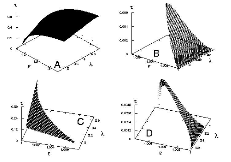
Figure 7: The ratio of the analogue to Hawking temperature $\tau$ (vertical axis) as a function of the specific energy of the flow ${\cal E}$ and the specific angular momentum $\lambda$. The representative cases shown are: mono-transonic flow passing through the single inner type sonic point (A), mono-transonic flow passing through the single outer type sonic point (B), multi-transonic accretion passing through the inner sonic point (C), and multi-transonic accretion passing through the outer sonic point (D).

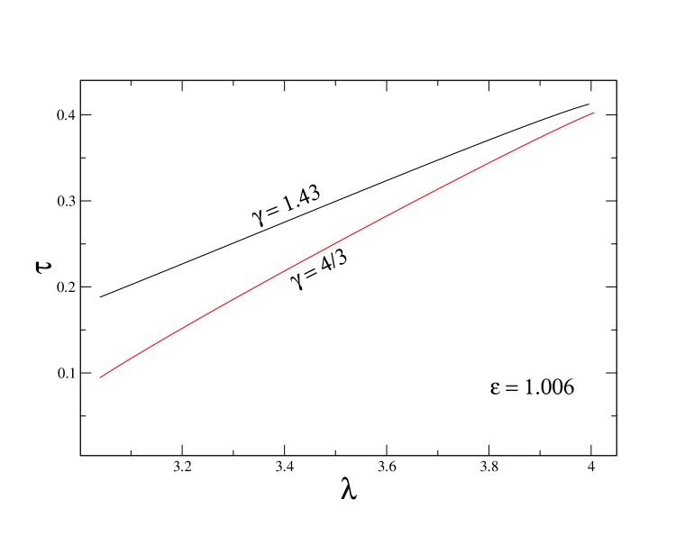
Figure 8: The ratio of the analogue to Hawking temperature $\tau$ as a function of specific angular momentum $\lambda$ for for a fixed specific energy ${\cal E}$ and two values of polytropic index $\gamma$.

VII Discussion

In this work, we have established that the general relativistic axisymmetric accretion disc round an astrophysical black hole can be considered as an example of classical analogue gravity realized in nature. To accomplish this task, we have first formulated and solved the equations describing the general relativistic axisymmetric accretion flow round a compact object. We then show that such accretion is transonic, and the collection of sonic points forms an acoustic horizon. The acoustic horizon is characterized by analogue surface gravity and the corresponding analogue Hawking radiation . We have calculated the corresponding analogue temperature as a function of fundamental accretion parameters. We have shown that for some region of parameter space spanned by the specific energy ${\cal E}$, the specific angular momentum $\lambda$ and the adiabatic index of the flow $\gamma$, the analogue Hawking temperature may exceed the Hawking temperature of the accreting black hole. Generally, this happens for high values of ${\cal E}$ and $\gamma$.

Note that the formalism presented in this work is not restricted to analogue effects in the black hole accretion only. Hydrodynamic accretion onto any astrophysical object, e.g. a weakly magnetized neutron star, if it happens to be transonic, will produce an acoustic horizon, and thus the analogue effects in such systems can be studied using the methodology developed here. Thus, we show in general, that a hydrodynamic transonic accretion in astrophysics may be regarded as a natural example of analogue gravity model.

It is important to note that the accreting astrophysical black holes are the only real physical candidates for which both the black-hole event hoizon and and the analogue sonic horizon may co-exist. Hence, our application of the analogue Hawking effect to the theory of transonic astrophysical accretion may be useful to compare the properties of these two types of horizons.

However, in our work, the analogy has been applied to describe the classical perturbation of the fluid in terms of a field satisfying the wave equation in an effective geometry. It is not our aim to provide a formulation by which the phonon field generated in this system could be quantized. To accomplish this task, one would need to show that the effective action for the acoustic perturbation is equivalent to a field theoretical action in curved space, and the corresponding commutation and dispersion relations should directly follow (see, e.g. stuz ). Such considerations are beyond the scope of this paper. Also note that for all types of accretion discussed here, the analogue temperature $T_{\rm AH}$ is many orders of magnitude lower compared with the fluid temperature of accreting matter.

In constructing a model for the disc height we have followed Abramowicz et al. discheight , although a number of other models for the disc height exist in the literature nt73 ; riffert ; pariev ; peitz ; lasota . The use of any other disc height model would not alter our conclusion that black-hole accretion disc solutions form an important class of analogue gravity models. However, the numerical values of $T_{AH}$ and other related quantities would be different for different disc heights.

In this work, the viscous transport of the angular momentum is not explicitly taken into account. Viscosity, however, is quite a subtle issue in studying the analogue effects for disc accretion. Thirty two years after the discovery of standard accretion disc theory nt73 ; ss73 , exact modeling of viscous transonic black-hole accretion, including proper heating and cooling mechanisms, is still quite an arduous task, even for a Newtonian flow. On the other hand, from the analogue model point of view, viscosity is likely to destroy Lorenz invariance, and hence the assumptions behind building up an analogue model may not be quite consistent. Nevertheless, extremely large radial velocity close to the black hole implies $\tau_{inf}\ll\tau_{visc}$, where $\tau_{inf}$ and $\tau_{visc}$ are the infall and the viscous time scales, respectively. Large radial velocities even at larger distances are due to the fact that the angular momentum content of the accreting fluid is relatively low belo ; igubelo ; proga . Hence, our assumption of inviscid flow is not unjustified from an astrophysical point of view. However, one of the most significant effects of the introduction of viscosity would be the reduction of the angular momentum. We found that the location of the sonic points anti-correlates with $\lambda$, i.e. weakly rotating flow makes the dynamical velocity gradient steeper, which indicates that for viscous flow the acoustic horizons will be pushed further out and the flow would become supersonic at a larger distance for the same set of other initial boundary conditions.

In our model, we have performed the computation of $T_{AH}$ for non-rotating black holes. Recently, the spacetime geometry on the equatorial slice through a Kerr black hole has been shown to be equivalent to the geometry experienced by phonons in a rotating fluid vortex silke . Since many astrophysical black holes are expected to possess non-zero spin (the Kerr parameter $a$), a clear understanding of the influence of spin on analogue models will be of great importance. Our initial calculation indicates that the black-hole spin enhances the analogue effect, i.e. the analogue Hawking temperature increases with the Kerr parameter $a$.

In connection to the acoustic geometry, one can define an ‘anti-trapped surface’ to be a hypersurface in which the fluid flow will be outward directed with the normal component of the three-velocity greater than the local speed of sound. In stationary geometry, an anti-trapped surface will naturally be constructed by the collection of sonic points corresponding to a spherically symmetric or axisymmetric transonic wind solution emanating out from an astrophysical source. Transonic outflow (wind) is ubiquitous in astrophysics, spanning a wide range from solar/stellar winds to large-scale outflows from active galaxies, quasars, galactic micro-quasars and energetic gamma ray bursts (GRB). In section III, we have shown how to identify the critical and the sonic points corresponding to the wind solutions. Such a formalism can be useful in studying the transonic properties of outflow from astrophysical sources. Hence our formalism presented in this paper can be applied to study the analogue effects in transonic winds as well. Recently Kinoshita et al.  kinoshita performed the causality analysis of the spherical GRB outflow using the concept of effective acoustic geometry. Such an investigation can be extended into a more robust form by incorporating our work to study the causal structure of the transonic GRB outflows in axisymmetry, i.e. for energetic directed outflow originating from a black-hole accretion disc system progenitor.

In recent years, considerable attention has been focused on the study of gravitational collapse of massive matter clump, in particular, on the investigation of the final fate of such collapse (for a review see, e.g. krolak ). Goswami and Joshi panu have studied the role of the equation of state and initial data in determining the final fate of the continual spherical collapse of barotropic fluid in terms of naked singularities and the black-hole formation. It is tempting to study the analogue effects in such a collapse model. Since at some stage the velocity of the collapsing fluid will exceed the velocity of local acoustic perturbation one might encounter a sonic horizons at the radial locations of the corresponding transonic points in a stationary configuration. One should, however, be careful about the issue that many results in analogue models are based on the assumption of a stationary flow, whereas a collapse scenario is a full time dependent dynamical process.

The correspondence between general relativity and analogue gravity has so far been exploited only on a kinematical, i.e. geometrical level. The analogue gravity systems lack a proper dynamical scheme, such as Einstein’s field equations in general relativity and hence the analogy is not complete. A certain progress in this direction has recently been made by Cadoni and Mignemi cadoni ; mignemi who have established a dynamical correspondence between analogue and dilaton gravity in 1+1 dimensions. We believe that our approach in which an arbitrary background geometry serves as a source for fluid dynamics may shed a new light towards a full analogy between general relativity and analogue gravity.

Appendix A Derivation of the acoustic wave equation

This derivation is based in part on references landau ; visser . The continuity and Euler’s equations may be expressed as:

$$\frac{\partial{\rho}}{\partial{t}}+{\nabla}\cdot\left(\rho{\vec{u}}\right)$$ (89)

$$\rho\frac{d{\vec{u}}}{dt}{\equiv}\rho\left[\frac{\partial{\vec{u}}}{\partial{t}}+\left({\vec{u}}\cdot{\nabla}\right){\vec{u}}\right]=-\nabla{p}+{\vec{F}}$$ (90)

with ${\vec{F}}$ being the sum of all external forces acting on the fluid wich may be expressed in terms of a potential

$${\vec{F}}=-{\rho}{\nabla}{\Phi},$$ (91)

Euler’s equation may now be recast in the form

$$\frac{\partial{\vec{u}}}{\partial{t}}={\vec{u}}\times(\nabla\times{\vec{u}})-{1\over\rho}\nabla p-\nabla\left({{1\over 2}}u^{2}+\Phi\right)$$ (92)

Next we assume the fluid to be inviscid, irrotational, and barotropic. Introducing the specific enthalpy $h$ such that

$${\nabla}h=\frac{\nabla{p}}{\rho}$$ (93)

and the velocity potential $\psi$ for which ${\vec{u}}=-{\nabla}\psi$, Eq. (92) may be writen as

$$-\frac{\partial{\psi}}{\partial{t}}+h+{1\over 2}(\nabla\psi)^{2}+\Phi=0$$ (94)

One now linearizes the continuity and Euler’s equation around some unperturbed background flow variables $\rho_{0}$, $p_{0}$, $\psi_{0}$. Introducing

$$\rho=\rho_{0}+\epsilon\rho_{1}+{\cal O}(\epsilon^{2}), p=p_{0}+\epsilon p_{1}+{\cal O}(\epsilon^{2}),$$

$$\psi=\psi_{0}+\epsilon\psi_{1}+{\cal O}(\epsilon^{2}), h=h_{0}+\epsilon h_{1},$$ (95)

from the continuity equation we obtain

$$\frac{\partial\rho_{0}}{\partial{t}}+\nabla\cdot(\rho_{0}\;{\vec{u}}_{0})=0;\;\;\;\;\;\frac{\partial\rho_{1}}{\partial{t}}+\nabla\cdot(\rho_{1}\;{\vec{u}}_{0}+\rho_{0}\;{\vec{u}}_{1})=0.$$ (96)

Equation (93) implies

$$h_{1}=p_{1}\frac{dh}{dp}=\frac{p_{1}}{\rho_{0}}\,.$$ (97)

Using this the linearized Euler equation reads

$$-\frac{\partial{\psi_{0}}}{\partial{t}}+h_{0}+{1\over 2}(\nabla\psi_{0})^{2}+\Phi=0;\;\;\;\;\;-\frac{\partial{\psi_{0}}}{\partial{t}}+{p_{1}\over\rho_{1}}-{\vec{u}}_{0}\cdot\nabla\psi_{1}=0.$$ (98)

Re-arrangement of the last equation together with the barotropic assumption yields

$$\rho_{1}={\partial\rho\over\partial p}\;p_{1}={\partial\rho\over\partial p}\;\rho_{0}\;(\partial_{t}\psi_{1}+{\vec{u}}_{0}\cdot\nabla\psi_{1})\,.$$ (99)

Substitution of this into the linearized continuity equation gives the sound wave equation

$$-\frac{\partial}{\partial{t}}\left[{\partial\rho\over\partial p}\;\rho_{0}\;\left(\frac{\partial\psi_{1}}{\partial{t}}+{\vec{u}}_{0}\cdot\nabla\psi_{1}\right)\right]+\nabla\cdot\left[\rho_{0}\;\nabla\psi_{1}-{\partial\rho\over\partial p}\;\rho_{0}\;{\vec{v}}_{0}\;\left(\frac{\partial\psi_{1}}{\partial{t}}+{\vec{v}}_{0}\cdot\nabla\psi_{1}\right)\right]=0.$$ (100)

Next, we define the local speed of sound by

$$c_{s}^{2}={\partial{p}}/{\partial\rho},$$ (101)

where the partial derivative is taken at constant specific entropy. With help of the $4\times{4}$ matrix

$$f^{\mu\nu}\equiv{\rho^{0}}\left[\matrix{-{I}&\vdots&-{\vec{u}}\cr\cdots\cdots&\cdot&\cdots\cdots\cdots\cdots\cr-{\vec{u}}&\vdots&(c_{s}^{2}-{{u}^{2}})\cr}\right]$$ (102)

where ${I}$ is the $3\times 3$ identity matrix, one can put Eq. (100) to the form

$${\partial}_{\mu}\left(f^{\mu{\nu}}{\partial}_{\nu}{\psi_{1}}\right)=0.$$ (103)

References

- (1) Barcelo, C., Liberati, S., and Visser, M., 2005, ‘Analogue Gravity’, Living Reviews in Relativity, Vol. 8, no. 12, websource http://relativity.livingreviews.org/Articles/lrr-2005-12/, also at gr-qc/0505065
- (2) Cardoso, V., 2005, Acoustic black holes, physics/0503042
- (3) Novello, Visser & Volovik (ed.) 2002, Artificial Black Holes. World Scientific, Singapore.
- (4) Unruh, W. G. 1981, Phys. Rev. Lett. 46, 1351
- (5) Jacobson, T. A. 1991, Phys. Rev. D. 44, 1731
- (6) Unruh, W. G. 1995, Phys. Rev. D. 51, 2827
- (7) Visser, M. 1998, Class. Quant. Grav. 15, 1767
- (8) Jacobson, T. A. 1999, Prog. Theor. Phys. Suppl. 136, 1
- (9) Bili, N. 1999, Class. Quant. Grav. 16, 3953
- (10) Bondi, H. 1952, MNRAS, 112, 195
- (11) Moncrief, V. 1980, ApJ. 235, 1038
- (12) Anderson, M. 1989, MNRAS, 239, 19
- (13) Das, T. K. 2004, Class. Quant. Grav. 21, 5253
- (14) Dasgupta, S., Bili, N., and Das, T. K., 2005, General Relativity & Gravitation (GRG), Volume 37, Number 11, 1877-1890
- (15) Abraham, H., Bilić, N., & Das, T. K., 2006, Class. Quant. Grav. 23, 2371
- (16) Bardeen, J. M., Press, W. H., & Teukolsky, S. A. 1972, ApJ, 178, 347
- (17) Novikov, I., & Thorne, K. S. 1973, in Black Holes,eds. c. De Witt and B. De Witt(Gordon and Breach, New York).
- (18) Abramowicz, M. A., & Zurek, W. H. 1981, ApJ, 246, 314
- (19) Matsumoto, R., Kato. S., Fukue. J., & Okazaki. A. T. 1984, PASJ, 36, 71
- (20) Lu, J. F. 1985, A & A, 148, 176
- (21) Muchotrzeb-Czerny, B. 1986, Acta Astronomica, 36, 1.
- (22) Fukue, J. 1987, PASJ, 39, 309
- (23) Abramowicz, M. A., & Kato, S., 1989, ApJ, 336, 304
- (24) Chakrabarti, S. K. 1989, ApJ, 347, 365
- (25) Yang, R., & Kafatos, M. 1995, A & A, 295, 238
- (26) Pariev, V. I. 1996, MNRAS, 283, 1264
- (27) Peitz, J. & Appl, S. 1997, MNRAS, 286, 681
- (28) Lu, J. F., Yu, K. N., Yuan, F., & Young, E. C. M. 1997, A & A, 321, 665
- (29) Das, T. K. 2002, ApJ, 577, 880
- (30) Das, T. K. 2004, MNRAS, 375, 384
- (31) Illarionov, A.F., & Sunyaev, R. A. 1975a, A & A, 39, 205
- (32) Liang, E. P. T., & Nolan, P. L. 1984, Space Sci. Rev., 38, 353
- (33) Bisikalo, A. A., Boyarchuk, V. M., Chechetkin, V. M., Kuznetsov, O. A., & Molteni, D. 1998, MNRAS, 300, 39
- (34) Illarionov, A. F. 1988, Soviet Astron., 31, 618
- (35) Ho, L. C. 1999, in Observational Evidence For Black Holes in the Universe, ed. S. K. Chakrabarti (Dordrecht: Kluwer), 153
- (36) Igumenshchev, I. V. & Abramowicz, M. A. 1999, MNRAS, 303, 309
- (37) Boyer, R. H., & Lindquist, R. W. 1967, J. Math. Phys. 8, 265
- (38) Manmoto, T. 2000, ApJ, 534, 734
- (39) Abramowicz, M. A., Lanza, A., & Percival, M. J. 1997, ApJ, 479, 179
- (40) Ferrari, A., Trussoni, E., Rosner, R., and Tsinganos, K. 1985, ApJ, 294, 397
- (41) Paczyński, B., & Wiita, P. J. 1980, A & A, 88, 23
- (42) Frank, J., King, A. R. & Raine, D. J. 1992, Accretion Power in Astrophysics (2nd ed.; Cambridge: Cambridge Univ.Press)
- (43) Parker, E. N., 1965, Space Science Reviews, vol. 4, p.666.
- (44) Jordan, D. W., & Smith, P. 1999, ‘Nonlinear ordinary differential equations: An introduction to dynamical systems’, Oxford University Press, USA, 3rd edition, October 21, 1999.
- (45) Bray, A. J., & Moore, M. A. 1987, Phys. rev. Lett. 58, 57
- (46) Bhattacharjee, J. K., Das, T. K., & Nag, S. ‘Chaotic behaviour in transonic black hole accretion’, in preperation.
- (47) Miller, R. C. (ed.) & Wiita, P. J. (ed), 1991, ‘Variability of Active Galactic Nuclei’, Cambridge University Press.
- (48) Landau, L. D., & Lifshitz, E. D. 1959, Fluid Mechanics, New York: Pergamon
- (49) Das, T. K., Pendharkar, J. K., & Mitra, S. 2003, ApJ, 592, 1078
- (50) Fukumura, K., & Tsuruta, S., 2004, ApJ, 611, 964
- (51) Das, T. K., & Chakrabarti, S. K. 1999, Class. Quantum Grav. 16, 3879
- (52) Das, T. K., Rao, A. R., & Vadawale, S. R. 2003, MNRAS, 343, 443
- (53) Moscibrodzka, M., Das, T. K., & Czerny, B. 2006, ‘The pattern of accretion flow onto Sgr A∗’, submitted to MNRAS.
- (54) Misner, C. W., Thorne, K. S., & Wheeler, J. A., 1973, Gravitation (San Francisco, CA: Freeman)
- (55) Wald, R. M., 1984, General Relativity (Chicago, IL: University of Chicago Press)
- (56) Barceló, C., Liberati, S., Sonego, S., & Visser, M., 2004, New J. Phys. 6 186, gr-qc/0408022
- (57) Birrell, N. D., & Davies, P. C. W. 1982, Quantum fields in curved space, Cambridge University Press, Cambridge.
- (58) Unruh, W. G. & Schtzhold, R. 2003, Phys. Rev. D. 68, 024008
- (59) Jacobson, T. 1991, Phis. Rev. D 44, 1731; 1992, Phys. Rev. D 48, 728; Corley, S., & Jacobson, T. 1996, Phys. Rev. D 54, 1568.
- (60) Riffert, H., & Herold, H. 1995, ApJ, 450, 508
- (61) Lasota, J. P., & Abramowicz, M. A. 1997, Class. Quantum Grav. 14, A237
- (62) Shakura, N. I., & Sunyaev, R. A. 1973, A & A, 24, 337
- (63) Beloborodov, A. M., & Illarionov, A. F. 1991, MNRAS, 323, 167
- (64) Igumenshchev, I. V., & Beloborodov, A. M., 1997, MNRAS, 284, 767
- (65) Proga, D., & Begelman, M. C., 2003, ApJ, 582, 69
- (66) Visser, M. & Weinfurtner, S., 2005, Class. Quant. Grav. 22, 2493
- (67) Artemova, I. V., Björnsson, G., & Novikov, I. D. 1996, ApJ, 461, 565
- (68) Nowak, A. M., & Wagoner, R. V. 1991, ApJ, 378, 656
- (69) Kinoshita, S., Sendouda, Y., & Takahashi, K., 2004, Phys. Rev. D., 70, 123006
- (70) Krolak, A., 1999, Progress of Theoretical Physics Supplement, 136, 45
- (71) Goswami, R., & Joshi, P., 2004, Class. Quant. Grav. 21, 3645
- (72) Cadoni, M., 2005, Class. Quant. Grav. 22, 409
- (73) Cadoni, M., & Mignemi, S., 2005, Acoustic analogues of black hole singularities, Phys. Rev. D 72, 084012, gr-qc/0504143.