Exact Analytic Spectrum of Relic Gravitational Waves in Accelerating Universe

Abstract

An exact analytic calculation is presented for the spectrum of relic gravitational waves in the scenario of accelerating Universe $\Omega_{\Lambda}+\Omega_{m}=1$. The spectrum formula contains explicitly the parameters of acceleration, inflation, reheating, and the (tensor/scalar) ratio, so that it can be employed for a variety of cosmological models. We find that the spectrum depends on the behavior of the present accelerating expansion. The amplitude of gravitational waves for the model $\Omega_{\Lambda}=0.65$ is about $\sim 50\%$ greater than that of the model $\Omega_{\Lambda}=0.7$, an effect accessible to the designed sensitivities of LIGO and LISA. The spectrum sensitively depends on the inflationary models with $a(\tau)\propto|\tau|^{1+\beta}$, and a larger $\beta$ yields a flatter spectrum, producing more power. The current LIGO results rule out the inflationary models of $\beta\geq-1.8$. The LIGO with its design sensitivity and the LISA will also be able to test the model of $\beta=-1.9$. We also examine the constraints on the spectral energy density of relic gravitational waves. Both the LIGO bound and the nucleosynthesis bound point out that the model $\beta=-1.8$ is ruled out, but the model $\beta=-2.0$ is still alive. The exact analytic results also confirm the approximate spectrum and the numerical one in our previous work.

I Introduction

Recently much progress has been made in the Laser Interferometer Gravitational waves Observatory (LIGO) with the typical sensitivity $10^{-22}$ to $10^{-23}$ being reached in the frequency range $100\sim 1000$Hz abbott r-abbott b-abbott1 b-abbott2 . The chance to detect directly the gravitational waves (GW) has thus increased. Therefore, it is necessary to examine the possible objects of detections, such as the relic GW, which has a spectrum distributed over a rather broad range of frequencies. The stochastic background of relic GW has long been studied starobinsky rubakov harari . The calculations of spectrum generated during the transitions from the inflationary era to the radiation-dominated era, or, to the matter-dominated era, have been carried out allen sahni grishchuk maia riazuelo tashiro henriques . More recently, studies has been made on the effects of the detailed slow-roll inflationary on the relic GW gong ungarelli smith , and on the other post-inflationary physical effects on the relic GW boyle . A constraint on the the tensor-to-scalar ratio $r$ has been derived, using the CMB-galaxy cross-correlation cooray . The relic GW can influence CMB and cause magnetic type of CMB polarizations, which can serve as another distinct signal of the relic GW. This kind of effects have been studied in Refs. Hu ; zalda ; kami ; keat ; zhz . On both theoretical and observational issues of the relic GW, a recent review is given by Grishchuk r-grishchuk .

The observations on the SN Ia riess perlmutter indicate that the Universe is currently under accelerating expansion, which may be driven by the cosmic dark energy ($\Omega_{\Lambda}\sim 0.7$) plus the dark matter ($\Omega_{m}\sim 0.3$) with $\Omega_{\Lambda}+\Omega_{m}=1$ bahcall spergel zhy . The evolution of relic GW after being generated during the inflationary stage depends on the subsequent expansion behaviors of the spacetime background. The current accelerating expansion of Universe will have an impact on the relic GW and its spectrum. The spectrum of relic GW has been studied in specific models for dark energy, such as the Chaplyngin gas model fbris and the X-fluid model santos . In previous study we have studied the effects on the relic GW caused by the acceleration of the Universe for fixed $\Omega_{\Lambda}=0.7$ and $\Omega_{m}=0.3$, and have obtained an approximate zh , and a numerical spectrum zh2 of the relic GW. It was shown that, in comparison with the decelerating models, both the shape and amplitude of the spectrum have been modified due to the current accelerating expansion. However, in the previous work, the dependence of the spectrum upon the dark energy fraction $\Omega_{\Lambda}$ has not been examined. Extending these previous studies, in this paper we present an exact analytic calculation of the spectrum for any fraction $\Omega_{\Lambda}$ of the dark energy. We will demonstrate how $\Omega_{\Lambda}$ affects the spectrum, discuss the dependence of spectrum upon the inflationary models. We will also examine the resulting spectrum by comparing with the sensitivity curves of the gravitational wave detections, such as the LIGO and LISA, and constrain the corresponding spectral energy density by the resent LIGO bound and by the nucleosynthesis bound. The resulting formula of spectrum will contain explicitly the parameter for the dark energy, as well as the parameters for the inflationary expansion, the reheating, the initial normalization of the amplitude, and the ratio of (tensor/scalar), so that it can be quite general and can be used in other possible applications. In this way the paper is also to serve as a useful compilation. Thus we have also listed the main formulae and the relevant specifications involved in the calculation of the spectrum. Throughout the paper we adopt notations similar to that of grishchuk zh for convenience.

II Expansion Stages of the Universe

The overall expansion of the spatially flat Universe is described by the Robertson-Walker metric $ds^{2}=a^{2}(\tau)[d\tau^{2}-\delta_{ij}dx^{i}dx^{j}]$, where $\tau$ is the conformal time. The scalar factor $a(\tau)$ is given by the following for various stages.

The initial stage (inflationary)

$$a(\tau)=l_{0}\mid{\tau}\mid^{1+\beta},\,\,\,\,\,-\infty<\tau\leq\tau_{1},$$ (1)

where $1+\beta<0$, and $\tau_{1}<0$. The special case of $\beta=-2$ is the de Sitter expansion of inflation.

The reheating stage

$$a(\tau)=a_{z}(\tau-\tau_{p})^{1+\beta_{s}},\,\,\,\,\,\tau_{1}\leq\tau\leq\tau_{s}.$$ (2)

This stage is introduced to allow a general reheating epoch grishchuk zh .

The radiation-dominated stage

$$a(\tau)=a_{e}(\tau-\tau_{e}),\,\,\,\,\,\tau_{s}\leq\tau\leq\tau_{2}.$$ (3)

The matter-dominated stage

$$a(\tau)=a_{m}(\tau-\tau_{m})^{2},\,\,\,\,\,\tau_{2}\leq\tau\leq\tau_{E},$$ (4)

where $\tau_{E}$ is the time when the dark energy density $\rho_{\Lambda}$ is equal to the matter energy density $\rho_{m}$. The redshift $z_{E}$ at the time $\tau_{E}$ is given by $1+z_{E}=(\frac{\Omega_{\Lambda}}{\Omega_{m}})^{1/3}$. If the current values $\Omega_{\Lambda}\sim 0.7$ and $\Omega_{m}\sim 0.3$ are taken, then $1+z_{E}\sim 1.33$. For $\Omega_{\Lambda}\sim 0.65$ and $\Omega_{m}\sim 0.25$ , then $1+z_{E}\sim 1.23$ zh .

The accelerating stage (up to the present time $\tau_{H}$)

$$a(\tau)=l_{H}|\tau-\tau_{a}|^{-\gamma},\,\,\,\,\,\tau_{E}\leq\tau\leq\tau_{H},$$ (5)

where the parameter $\gamma=1.0$ is the de Sitter acceleration for $\Omega_{\Lambda}=1$ and $\Omega_{m}=0$. For the realistic model with $\Omega_{\Lambda}=0.7$ and $\Omega_{m}=0.3$ at present, we have numerically solved the Friedman equation

$$(\frac{a^{\prime}}{a^{2}})^{2}=H^{2}(\Omega_{\Lambda}+\Omega_{m}a^{-3})$$ (6)

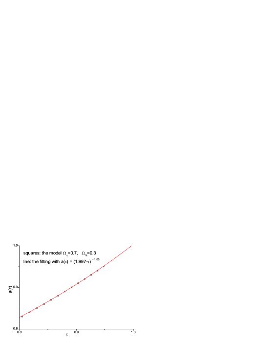
Figure 1: For the accelerating expansion with $\Omega_{\Lambda}=0.7$ the scale factor $a(\tau)$ can be fitted by Eq.(5) with the parameter $\gamma=1.05$.

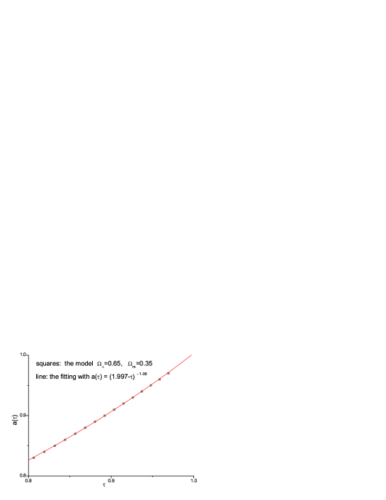
Figure 2: For the accelerating expansion with $\Omega_{\Lambda}=0.65$ the scale factor $a(\tau)$ can be fitted by Eq.(5) with $\gamma=1.06$.

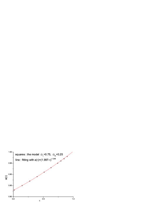
Figure 3: For the accelerating expansion with $\Omega_{\Lambda}=0.75$ the scale factor $a(\tau)$ can be fitted by Eq.(5) with $\gamma=1.048$.

where $a^{\prime}\equiv da(\tau)/d\tau$. The resulting $a(\tau)$ is plotted in Fig.1. We have found that the expression of (5) with $\gamma=1.05$ gives a good fitting to the numerical solution $a(\tau)$. Similar calculations show that $\gamma=1.06$ fits the model of $\Omega_{\Lambda}=0.65$ (in Fig.2), $\gamma=1.048$ fits the model $\Omega_{\Lambda}=0.75$ ( in Fig.3), and $\gamma=1.042$ fits the model $\Omega_{\Lambda}=0.80$. Thus, for the spatially flat Universe ($\Omega_{\Lambda}+\Omega_{m}=1$), as long as the dark energy dominates over the matter component ($\Omega_{\Lambda}>\Omega_{m}$), the generic fitting formula Eq.(5) is effectively valid, and the range of values for the parameter $\gamma$ are close to $1.0$. The constant $\tau_{a}$ in Eq.(5) can be taken to be the same value, not very sensitive to the various values of $\Omega_{\Lambda}$ and $\Omega_{m}$.

There are ten constants in the above expressions of $a(\tau)$, except $\beta$, $\beta_{s}$, and $\gamma$ , that are imposed upon as the model parameters. By the continuity conditions of $a(\tau)$ and $a(\tau)^{\prime}$ at the four given joining points $\tau_{1}$, $\tau_{s}$, $\tau_{2}$, and $\tau_{E}$, one can fix only eight constants. The other two constants can be fixed by the overall normalization of $a$ and by the observed Hubble constant as the expansion rate. Specifically, we put $a(\tau_{H})=l_{H}$ as the normalization, i.e.

$$|\tau_{H}-\tau_{a}|=1,$$ (7)

and the constant $l_{H}$ is fixed by the following calculation

$$\frac{1}{H}\equiv\left(\frac{a^{2}}{a^{\prime}}\right)_{\tau_{H}}=\frac{l_{H}}{\gamma}.$$ (8)

As we have shown that $\gamma\simeq 1.0$ in the realistic models of acceleration expansion, so $l_{H}$ is just the Hubble radius at present. Then everything in the expressions of $a(\tau)$ from Eq.(1) through Eq.(5) is fixed up. For instance, one obtains

$$l_{0}=l_{H}b\gamma\zeta_{E}^{-(1+\frac{1+\beta}{\gamma})}\zeta_{2}^{\frac{\beta-1}{2}}\zeta_{s}^{\beta}\zeta_{1}^{\frac{\beta-\beta_{s}}{1+\beta_{s}}},$$ (9)

where $b\equiv|1+\beta|^{-(1+\beta)}$, $\zeta_{E}\equiv\tau_{E}/\tau_{H}$, $\zeta_{2}\equiv(\tau_{E}/\tau_{2})^{2}$, $\zeta_{s}\equiv\tau_{2}/\tau_{s}$, and $\zeta_{1}\equiv(\tau_{s}/\tau_{1})^{1+\beta_{s}}$.

To completely fix the joining conditions we need to specify the time instants $\tau_{1}$, $\tau_{2}$, $\tau_{s}$, and $\tau_{E}$ that separate two consecutive expansion stages. From the consideration of physics of the Universe, we take the following specifications zh : $a(\tau_{H})/a(\tau_{E})=1.33$, $a(\tau_{E})/a(\tau_{2})=3454$, $a(\tau_{2})/a(\tau_{s})=10^{24}$, and $a(\tau_{s})/a(\tau_{1})=300$. From these, one makes use of the continuity conditions of $a$ and $a^{\prime}$, and obtains

$$|\tau_{E}-\tau_{a}|=(1+z_{E})^{\frac{1}{\gamma}},$$

$$|\tau_{E}-\tau_{m}|=\frac{2(1+z_{E})}{\gamma},$$

$$|\tau_{2}-\tau_{m}|=\frac{2(1+z_{E})}{\gamma\sqrt{3454}},$$

$$|\tau_{2}-\tau_{e}|=\frac{(1+z_{E})}{\gamma\sqrt{3454}},$$

$$|\tau_{s}-\tau_{e}|=\frac{(1+z_{E})\times 10^{-24}}{\gamma\sqrt{3454}},$$

$$|\tau_{s}-\tau_{p}|=(1+\beta_{s})\frac{(1+z_{E})\times 10^{-24}}{\gamma\sqrt{3454}},$$

$$|\tau_{1}-\tau_{p}|=\frac{(1+\beta_{s})}{300^{\frac{1}{\beta_{s}+1}}}\frac{(1+z_{E})\times 10^{-24}}{\gamma\sqrt{3454}},$$

$$|\tau_{1}|=\frac{|1+\beta|}{300^{\frac{1}{\beta_{s}+1}}}\frac{(1+z_{E})\times 10^{-24}}{\gamma\sqrt{3454}}.$$ (10)

The above expressions all depend on the model parameters $\beta$, $\beta_{s}$, and $\gamma$ explicitly, thus depend on $\Omega_{\Lambda}$. So we can expect that the spectrum of relic GW will depend on the present acceleration behavior of the Universe through $\gamma$.

In the expanding Robertson-Walker spacetime the physical wavelength $\lambda$ is related to the comoving wave number $k$ by

$$\lambda\equiv\frac{2\pi a(\tau)}{k}.$$ (11)

By Eq.(7) the wave number corresponding to the present Hubble radius is $k_{H}=2\pi a(\tau_{H})/l_{H}=2\pi$. There is another wave number, $k_{E}\equiv 2\pi a(\tau_{E})H=k_{H}/(1+z_{E})$, whose corresponding wavelength is the Hubble radius $1/H$ at the time $\tau_{E}$.

III Equation of Gravitational Waves

Incorporating the perturbations to the Robertson-Walker metric, one writes

$$ds^{2}=a^{2}(\tau)[d\tau^{2}-(\delta_{ij}+h_{ij})dx^{i}dx^{j}],$$ (12)

where $h_{ij}$ is $3\times 3$ symmetric, representing the perturbations. The gravitational wave field is the tensorial portion of $h_{ij}$, which is transverse-traceless $\partial_{i}h^{ij}=0$, $\delta^{ij}h_{ij}=0$, and the wave equation is

$$\partial_{\mu}(\sqrt{-g}\partial^{\mu}h_{ij}({\bf{x}},\tau))=0.$$ (13)

For a fixed wave vector $\bf k$ and a fixed polarization state $\sigma$, the wave equation reduces to the second-order ordinary differential equation zh grish

$$h_{k}^{(\sigma)^{\prime\prime}}+2\frac{a^{\prime}}{a}h_{k}^{(\sigma)^{\prime}}+k^{2}h^{(\sigma)}_{k}=0,$$ (14)

where the prime denotes $d/d\tau$. Since the equation of $h_{\bf k}^{(\sigma)}(\tau)$ for each polarization $\sigma$ is the same, we denote $h_{\bf k}^{(\sigma)}(\tau)$ by $h_{\bf k}(\tau)$ in the following. Once the mode function $h_{k}(\tau)$ is known, the spectrum $h(k,\tau)$ of relic GW is given by

$$h(k,\tau)=\frac{4l_{Pl}}{\sqrt{\pi}}k|h_{k}(\tau)|,$$ (15)

which is defined by the following equation

$$\int^{\infty}_{0}h^{2}(k,\tau)\frac{dk}{k}\equiv<0|h^{ij}({\bf x},\tau)h_{ij}({\bf x},\tau)|0>,$$ (16)

where the right-hand-side is the vacuum expectation value of the operator $h^{ij}h_{ij}$. The spectral energy density parameter $\Omega_{g}(k)$ of the GW is defined through the relation

$$\frac{\rho_{g}}{\rho_{c}}=\int\Omega_{g}(k)\frac{dk}{k},$$

where $\rho_{g}=\frac{1}{32\pi G}h_{ij,\,0}h^{ij}_{\,\,,\,0}$ is the energy density of the GW, and $\rho_{c}$ is the critical energy density. Then, one reads

$$\Omega_{g}(k)=\frac{\pi^{2}}{3}h^{2}(k,\tau_{H})(\frac{k}{k_{H}})^{2},$$ (17)

which is dimensionless. Note that the there might be divergences in the integration for $\rho_{g}$, either infrared or ultraviolet. As is known, the infrared divergence is avoided if a infrared cutoff is introduced. This can be done since the very long waves with wavelengths comparable to, or longer than, the Hubble length do not contribute to the GW energy density zeldovich . As for the very short wavelength portion, the ultraviolet divergences is also avoided by considering the Parker’s adiabatic theorem parker2 , which states that, during a transition between expansion epochs with a characteristic time duration $\Delta t$, the gravitons created will be suppressed for wavenumbers $k>1/\Delta t$. Thus, the spectrum segments in both the very low and very high frequency ranges should be discarded from these physical considerations.

IV Initial Amplitude of Spectrum

Regarding to the relic GW, the initial conditions are taken to be during the inflationary stage. For a given wave number $k$, the corresponding wave crossed over the horizon at a time $\tau_{i}$, i.e. when the wave length was equal to the Hubble radius: $\lambda_{i}=2\pi a(\tau_{i})/k$ to $1/H(\tau_{i})$. From Eq.(1) yields $H(\tau_{i})=l_{0}^{-1}|1+\beta|\cdot|\tau_{i}|^{2+\beta}$, and, for the case of exact de Sitter expansion of $\beta=-2$, one has $H(\tau_{i})=l_{0}^{-1}$. Thus a different $k$ corresponds to a different time $\tau_{i}$. Now choose the initial condition of the mode function $h_{k}(\tau)$ as

$$|h_{k}(\tau_{i})|=\frac{1}{a(\tau_{i})}.$$ (18)

Then the initial amplitude of the spectrum is grishchuk zh

$$h(k,\tau_{i})=A(\frac{k}{k_{H}})^{2+\beta},$$ (19)

where the constant

$$A=8\sqrt{\pi}b\frac{l_{Pl}}{l_{0}}.$$ (20)

The power spectrum for the primordial perturbations of energy density is $P(k)\propto|h(k,\tau_{H})|^{2}$, and its spectral index $n$ is defined as $P(k)\propto k^{n-1}$. Thus one reads off the relation $n=2\beta+5$. The exact de Sitter expansion of $\beta=-2$ leads to $n=1$, yielding an initial spectrum independent of $k$, called the scale-invariant primordial spectrum. Other values of $\beta$ will differ from the scale-invariant one.

As is known, any calculation of the spectrum of the relic GW always has some overall uncertainty, originating from the normalization of the amplitude. Currently, from the observational perspective, the best that one can do is to use the CMB anisotropies to constrain the amplitude, as they receive the contributions from both the scalar (density) and the tensorial (GW) primordial perturbations. However, there is a well known problem of how much relative contribution is from the relic GW, in comparison with the scalar type contribution (the density perturbations). There have been a number of discussion on the ratio of the relic GW to the scalar contribution,

$$r=P_{h}/P_{s}.$$ (21)

Theoretically, it is, in our view, a problem of initial conditions on the ratio of the scalar and tensorial modes of comic perturbations. So far, in regards to the very long wavelength, some preliminary conclusion on the upper limit of GW contributions has been given, based upon the analysis on WMAP and the observational results of SDSS, for instance, $r<0.37$ (95% c.l.) Peiris Seljak . The final conclusion on this issue might be eventually rely on the more observations of CMB anisotropies and polarization (such as the Planck project in near future). In the following, the ratio $r$ is treated as a parameter, representing the relative contribution by the relic GW to the CMB anisotropies $\Delta T/T$ at low multipoles. This will determine the overall factor $A$ in (19). Using the observed CMB anisotropies spergel is $\Delta T/T\simeq 0.37\times 10^{-5}$ at $l\sim 2$, which corresponds to the anisotropies on the scale of Hubble radius, we put

$$h(k_{H},\tau_{H})=0.37\times 10^{-5}r.$$ (22)

Then the spectrum $h(k,\tau_{H})$ at the present time $\tau_{H}$ is fixed. If we take the upper limit $r=0.37$, then $h(k_{H},\tau_{H})\simeq 0.14\times 10^{-5}$. For smaller $r$, our calculation is still similar except the resulting spectrum is reduced by the corresponding numerical factor.

V Analytic Solution

Writing the mode function $h_{k}(\tau)=\mu_{k}(\tau)/a(\tau)$ in Eq.(14), the equation for $\mu_{k}(\tau)$ becomes

$$\mu^{\prime\prime}_{k}+(k^{2}-\frac{a^{\prime\prime}}{a})\mu_{k}=0.$$ (23)

For a scale factor of power-law form $a(\tau)\propto\tau^{\alpha}$, the general exact solution is of the following form

$$\mu_{k}(\tau)=c_{1}(k\tau)^{\frac{1}{2}}J_{\alpha-\frac{1}{2}}(k\tau)+c_{2}(k\tau)^{\frac{1}{2}}J_{\frac{1}{2}-\alpha}(k\tau),$$

where the constant $c_{1}$ and $c_{2}$ are to determined by continuity of the function $\mu_{k}(\tau)$ and the time derivative $(\mu_{k}(\tau)/a(\tau))^{\prime}$ at the time instance joining two consecutive stages.

The inflationary stage has the solution

$$\mu_{k}(\tau)=x^{\frac{1}{2}}[A_{1}J_{\beta+\frac{1}{2}}(x)+A_{2}J_{-(\beta+\frac{1}{2})}(x)],\,\,\,\,-\infty<\tau\leq\tau_{1},$$ (24)

where $x\equiv k\tau$, and the two constants $A_{1}$ and $A_{2}$, determining the initial states, are taken to be

$$A_{1}=-\frac{i}{\cos\beta\pi}\sqrt{\frac{\pi}{2}}e^{i\pi\beta/2},\,\,\,\,\,\,\,A_{2}=iA_{1}e^{-i\pi\beta},$$ (25)

both are independent of k. With Eq.(25) the mode function $\mu_{k}(\tau)$ is proportional to the Hankel’s function $H_{\beta+\frac{1}{2}}^{(2)}$,

$$\mu_{k}(\tau)=A_{1}e^{-i\pi\beta}\sin(\beta\pi+\frac{\pi}{2})x^{\frac{1}{2}}H_{\beta+\frac{1}{2}}^{(2)}(x),$$ (26)

which, in the high frequency limit, approaches to the positive frequency mode

$$\lim_{k\rightarrow\infty}\mu_{k}(\tau)\rightarrow e^{-ik\tau}.$$

Thus the initial state fixed by Eq.(25) corresponds to the so-called adiabatic vacuum in the high frequency limit parker bunch .

The reheating stage has

$$\mu_{k}(\tau)=t^{\frac{1}{2}}[B_{1}J_{\beta_{s}+\frac{1}{2}}(t)+B_{2}J_{-\beta_{s}-\frac{1}{2}}(t)],\,\,\,\,\,\,\tau_{1}<\tau\leq\tau_{s},$$ (27)

where the variable $t\equiv k(\tau-\tau_{p})$, and the two coefficients $B_{1}$ and $B_{2}$ are fixed by joining the functions $\mu_{k}(\tau)$ and $(\mu_{k}(\tau)/a(\tau))^{\prime}$ continuously at the time $\tau_{1}$ when the reheating epoch begins:

$$B_{1}=\sqrt{\frac{x_{1}}{t_{1}}}\frac{J_{\beta+\frac{1}{2}}(x_{1})J_{-\beta_{s}-\frac{3}{2}}(t_{1})+J_{\beta+\frac{3}{2}}(x_{1})J_{-\beta_{s}-\frac{1}{2}}(t_{1})}{J_{\beta_{s}+\frac{1}{2}}(t_{1})J_{-\beta_{s}-\frac{3}{2}}(t_{1})+J_{-\beta_{s}-\frac{1}{2}}(t_{1})J_{\beta_{s}+\frac{3}{2}}(t_{1})}A_{1}$$

$$+\sqrt{\frac{x_{1}}{t_{1}}}\frac{J_{-\beta-\frac{1}{2}}(x_{1})J_{-\beta_{s}-\frac{3}{2}}(t_{1})-J_{-\beta-\frac{3}{2}}(x_{1})J_{-\beta_{s}-\frac{1}{2}}(t_{1})}{J_{\beta_{s}+\frac{1}{2}}(t_{1})J_{-\beta_{s}-\frac{3}{2}}(t_{1})+J_{-\beta_{s}-\frac{1}{2}}(t_{1})J_{\beta_{s}+\frac{3}{2}}(t_{1})}A_{2},$$ (28)

$$B_{2}=\sqrt{\frac{x_{1}}{t_{1}}}\frac{J_{\beta+\frac{1}{2}}(x_{1})J_{\beta_{s}+\frac{3}{2}}(t_{1})-J_{\beta+\frac{3}{2}}(x_{1})J_{\beta_{s}+\frac{1}{2}}(t_{1})}{J_{\beta_{s}+\frac{1}{2}}(t_{1})J_{-\beta_{s}-\frac{3}{2}}(t_{1})+J_{-\beta_{s}-\frac{1}{2}}(t_{1})J_{\beta_{s}+\frac{3}{2}}(t_{1})}A_{1}$$

$$+\sqrt{\frac{x_{1}}{t_{1}}}\frac{J_{-\beta-\frac{3}{2}}(x_{1})J_{\beta_{s}+\frac{1}{2}}(t_{1})+J_{-\beta-\frac{1}{2}}(x_{1})J_{\beta_{s}+\frac{3}{2}}(t_{1})}{J_{\beta_{s}+\frac{1}{2}}(t_{1})J_{-\beta_{s}-\frac{3}{2}}(t_{1})+J_{-\beta_{s}-\frac{1}{2}}(t_{1})J_{\beta_{s}+\frac{3}{2}}(t_{1})}A_{2}$$ (29)

with $x_{1}\equiv k\tau_{1}$, $t_{1}\equiv k(\tau_{1}-\tau_{p})$, and $(1+\beta_{s})x_{1}=(1+\beta)t_{1}$, which follows from the continuity of $a(\tau)$ and $a^{\prime}(\tau)$ at the time $\tau_{1}$.

The radiation-dominated stage has

$$\mu_{k}(\tau)=C_{1}e^{-iy}+C_{2}e^{iy},\,\,\,\,\,\,\,\,\tau_{s}\leq\tau\leq\tau_{2},$$ (30)

where the variable $y\equiv k(\tau-\tau_{e})$, and $C_{1}$ and $C_{2}$ are given by

$$C_{1}=\frac{e^{iy_{s}}t_{s}^{\frac{1}{2}}}{2i}\left\{[(i-\frac{1}{y_{s}})J_{\beta_{s}+\frac{1}{2}}(t_{s})+J_{\beta_{s}+\frac{3}{2}}(t_{s})]B_{1}+[(i-\frac{1}{y_{s}})J_{-\beta_{s}-\frac{1}{2}}(t_{s})-J_{-\beta_{s}-\frac{3}{2}}(t_{s})]B_{2}\right\},$$ (31)

$$C_{2}=\frac{-e^{-iy_{s}}t_{s}^{\frac{1}{2}}}{2i}\left\{[-(i+\frac{1}{y_{s}})J_{\beta_{s}+\frac{1}{2}}(t_{s})+J_{\beta_{s}+\frac{3}{2}}(t_{s})]B_{1}+[-(i+\frac{1}{y_{s}})J_{-\beta_{s}-\frac{1}{2}}(t_{s})-J_{-\beta_{s}-\frac{3}{2}}(t_{s})]B_{2}\right\},$$ (32)

where $t_{s}\equiv k(\tau_{s}-\tau_{p})$, $y_{s}\equiv k(\tau_{s}-\tau_{e})$, and $t_{s}=(1+\beta_{s})y_{s}$.

The matter-dominated stage has

$$\mu_{k}(\tau)=\sqrt{\frac{\pi z}{2}}[D_{1}J_{\frac{3}{2}}(z)+D_{2}J_{-\frac{3}{2}}(z)],\,\,\,\,\,\tau_{2}\leq\tau\leq\tau_{E},$$ (33)

where $z\equiv k(\tau-\tau_{m})$, and $D_{1}$ and $D_{2}$ are given by

$$D_{1}=[-e^{iy_{2}}-\frac{i}{2y_{2}}e^{iy_{2}}+\frac{e^{iy_{2}}+e^{-3iy_{2}}}{8y_{2}^{2}}]C_{1}+[-e^{-iy_{2}}+\frac{i}{2y_{2}}e^{-iy_{2}}+\frac{e^{-iy_{2}}+e^{3iy_{2}}}{8y^{2}_{2}}]C_{2},$$ (34)

$$D_{2}=[ie^{iy_{2}}-\frac{e^{iy_{2}}}{2y_{2}}-\frac{i}{8y_{2}^{2}}(e^{iy_{2}}-e^{-3iy_{2}})]C_{1}-[ie^{-iy_{2}}+\frac{e^{-iy_{2}}}{2y_{2}}+\frac{i}{8y_{2}^{2}}(e^{3iy_{2}}-e^{-iy_{2}})]C_{2},$$ (35)

with $y_{2}\equiv k(\tau_{2}-\tau_{e})$.

The accelerating stage has

$$\mu_{k}(\tau)=\sqrt{\frac{\pi s}{2}}[E_{1}J_{\gamma+\frac{1}{2}}(s)+E_{2}J_{-\gamma-\frac{1}{2}}(s)],\,\,\,\,\,\tau_{E}\leq\tau\leq\tau_{H},$$ (36)

where $s\equiv k(\tau-\tau_{a})$, and $E_{1}$ and $E_{2}$ are given by

$$E_{1}=\Delta^{-1}\frac{z_{E}}{s_{E}}\left\{J_{\frac{3}{2}}(z_{E})[-\frac{J_{-\gamma-\frac{1}{2}}(s_{E})}{s_{E}}-J_{-\gamma-\frac{3}{2}}(s_{E})]-J_{\frac{5}{2}}(z_{E})J_{-\gamma-\frac{1}{2}}(s_{E})\right\}D_{1}$$

$$+\left\{J_{-\frac{3}{2}}(z_{E})[-\frac{J_{-\gamma-\frac{1}{2}}(s_{E})}{s_{E}}-J_{-\gamma-\frac{3}{2}}(s_{E})]+J_{-\frac{5}{2}}(z_{E})J_{-\gamma-\frac{1}{2}}(s_{E})\right\}D_{2},$$ (37)

$$E_{2}=\Delta^{-1}\frac{z_{E}}{s_{E}}\left\{J_{\frac{5}{2}}(z_{E})J_{\gamma+\frac{1}{2}}(s_{E})-J_{\frac{3}{2}}[-\frac{J_{\gamma+\frac{1}{2}}}{s_{E}}(s_{E})+J_{\gamma+\frac{3}{2}}(s_{E})]\right\}D_{1}$$

$$+\left\{-J_{-\frac{5}{2}}(z_{E})J_{\gamma+\frac{1}{2}}(s_{E})-J_{-\frac{3}{2}}[-\frac{J_{\gamma+\frac{1}{2}}}{s_{E}}(s_{E})+J_{\gamma+\frac{3}{2}}(s_{E})]\right\}D_{2}.$$ (38)

$$\Delta=J_{\gamma+\frac{1}{2}}(s_{E})[-\frac{J_{-\gamma-\frac{1}{2}}(s_{E})}{s_{E}}-J_{-\gamma-\frac{3}{2}}(s_{E})]-J_{-\gamma-\frac{1}{2}}(s_{E})[-\frac{J_{\gamma+\frac{1}{2}}(s_{E})}{s_{E}}+J_{\gamma+\frac{3}{2}}(s_{E})]$$ (39)

where $z_{E}\equiv k(\tau_{E}-\tau_{m})$, $s_{E}\equiv k(\tau_{E}-\tau_{a})$, and $\gamma z_{E}=-2s_{E}$.

With all these coefficients having been fixed, the mode function $h_{k}(\tau_{H})$ is known as a function of the wave number $k$ at present time $\tau_{H}$, so is the spectrum

$$h(k,\tau_{H})=\frac{4l_{Pl}}{\sqrt{\pi}}k|h_{k}(\tau_{H})|,$$ (40)

as defined in Eq.(15). The above results form a useful compilation for computing the relic GW. To make use of the formulation (40), one substitutes $h_{k}(\tau_{H})=\mu_{k}(\tau_{H})/a(\tau_{H})$, where $\mu_{k}(\tau_{H})$ is given in Eq.(36). Of course, to specify $\mu_{k}(\tau_{H})$, all the coefficients $E_{1}$ , $E_{2}$ throughout $A_{1}$, $A_{2}$ have to be employed. One may, in his own computation, choose proper values of the parameters $\beta$, $\beta_{s}$, and $\gamma$ for the specific expansion behavior, as well as the initial amplitude $A$ in Eq.(22).

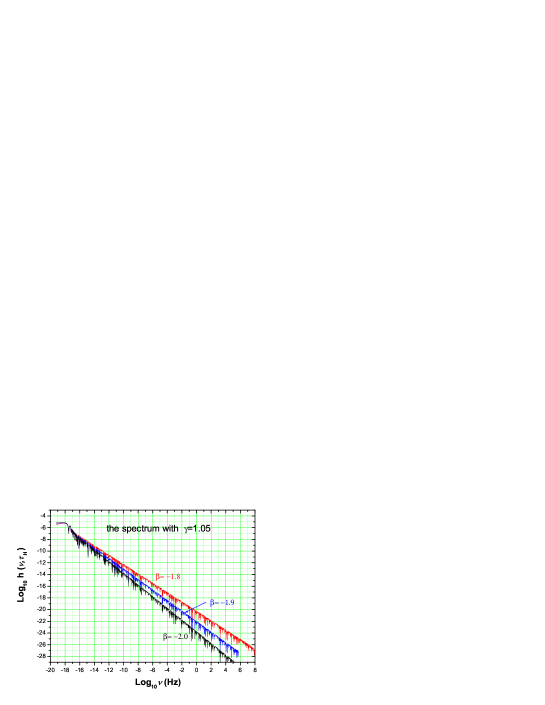
Figure 4: For a fixed acceleration parameter $\gamma=1.05$ the exact spectrum $h(\nu,\tau_{H})$ is plotted for three inflationary models of $\beta=-1.8$, $\beta=-1.9$, and $\beta=-2.0$, respectively.

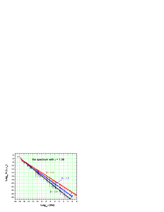
Figure 5: For a fixed acceleration parameter $\gamma=1.06$ the exact spectrum $h(\nu,\tau_{H})$ is plotted for three inflationary models of $\beta=-1.8$, $\beta=-1.9$, and $\beta=-2.0$, respectively.

For illustrations, taking the (tensor/scalr) ratio in Eq.(21) $r=0.37$, we have plotted the exact spectrum $h(k,\tau_{H})$ as a function of the frequency $\nu=k/2\pi a$ in Fig.4 for $\gamma=1.05$, and in Fig.5 for $\gamma=1.06$. In each of these figures of fixed $\gamma$, three spectra are shown for three inflationary models with $\beta=-1.8,-1.9$, and $-2.0$, and the parameter $\beta_{s}=0.598$, $-0.552$, and $-0.689$ are taken, respectively zh . As these figures show, the spectrum is scale-invariant with a flat segment in the range $\nu\leq 10^{-18}$Hz and a slope segment in the range $\nu\geq 10^{-18}$Hz.

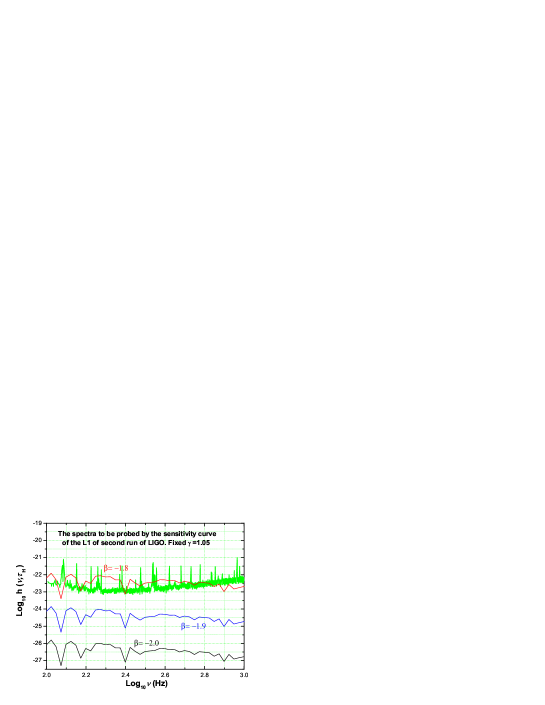
Figure 6: For a fixed acceleration parameter $\gamma=1.05$ the exact spectrum $h(\nu,\tau_{H})$ is plotted within the range of $\nu=10^{2}-10^{3}$Hz for three inflationary models of $\beta=-1.8$, $\beta=-1.9$, and $\beta=-2.0$, to compare with the sensitivity curve of second run from LIGO L1 b-abbott2 .

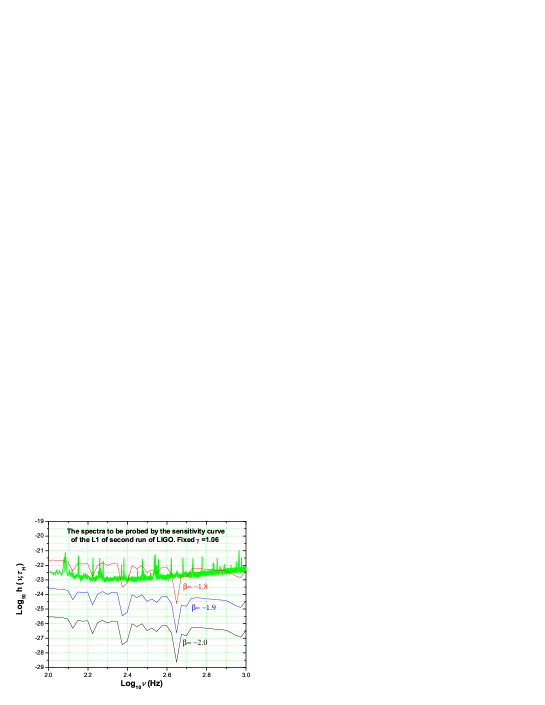
Figure 7: For a fixed acceleration parameter $\gamma=1.06$ the exact spectrum $h(\nu,\tau_{H})$ is plotted within the range of $\nu=10^{2}-10^{3}$Hz for three inflationary models of $\beta=-1.8$, $\beta=-1.9$, and $\beta=-2.0$, to compare with the sensitivity curve of second run from LIGO L1 b-abbott2 .

Now we make a comparison of the exact spectrum $h(\nu,\tau_{H})$ with the sensitivity curve from the recent S2 of LIGO abbott r-abbott b-abbott2 with the sensitivity $10^{-22}$ to $10^{-23}$ in the frequency range $\nu=10^{2}\sim 10^{3}$Hz. $h(\nu,\tau_{H})$ is given in Fig.6 for $\gamma=1.05$ and in Fig.7 for $\gamma=1.06$. Both figures have plotted three spectra for inflationary models $\beta=-1.8$, $\beta=-1.9$, and $\beta=-2.0$, respectively. It is found that the inflationary models with $\beta\geq-1.8$ has an amplitude about an order higher than the LIGO sensitive curve. Even if we take a much lower value for the (tensor/scalar) ratio, say $r=0.05$, the spectrum is still within the region detectable by the LIGO. Thus, the inflationary model $\beta=-1.8$ generating the relic GW with $r>0.05$ is ruled out by the LIGO null results. The models $\beta\leq-1.9$ are still alive by this test alone. Moreover, when LIGO reaches its design sensitivity $\sim 10^{-24}$ in the frequency range in the forthcoming runs, it will also be able to test the model of $\beta=-1.9$.

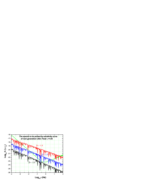
Figure 8: For a fixed acceleration parameter $\gamma=1.05$ the exact spectrum $h(\nu,\tau_{H})$ is plotted within the range of $\nu=10^{-4}-10^{2}$Hz for three inflationary models of $\beta=-1.8$, $\beta=-1.9$, and $\beta=-2.0$, to compare with the sensitivity from LISA the Next Generation lisa .

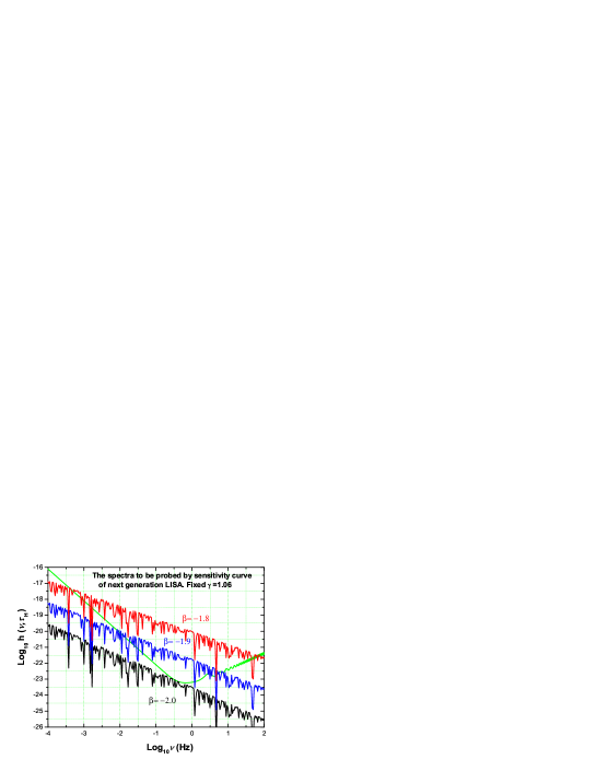
Figure 9: For a fixed acceleration parameter $\gamma=1.06$ the exact spectrum $h(\nu,\tau_{H})$ is plotted within the range of $\nu=10^{-4}-10^{2}$Hz for three inflationary models of $\beta=-1.8$, $\beta=-1.9$, and $\beta=-2.0$, to compare with the sensitivity from LISA the Next Generation lisa .

Fig.8 for $\gamma=1.05$ and Fig.9 for $\gamma=1.06$ give a comparison of the exact spectrum $h(\nu,\tau_{H})$ with the sensitivity curve from LISA the Next Generation lisa in the lower frequency range $\nu=10^{-4}\sim 10^{2}$Hz. It is interesting to notice that, when the LISA, as being designed, runs in space in the near future, it will be able to examine directly not only the model $\beta=-1.8$ but also the model $\beta=-1.9$. For the latter model, even if a much lower value of the ratio $r=0.05$ is taken, the LISA will still be able to detect it. This will be an improvement over the LIGO detection on the earth. However, as the two figures show, the inflationary model $\beta=-2.0$ seems to be still difficult to detect by the LISA with the capability as presently designed.

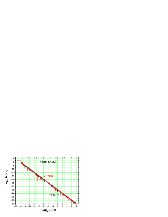
Figure 10: For a fixed inflationary parameter $\beta=-2.0$ the spectrum $h(\nu,\tau_{H})$ is plotted for different acceleration models of $\gamma=1.05$ and $\gamma=1.06$. The two spectra are quite close to each other, and the difference in amplitudes of $h(\nu,\tau_{H})$ is quite small, and difficult to tell in this figure.

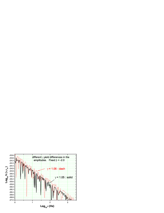
Figure 11: This enlarged picture is a portion of Fig.10 in the range $\nu=1-10^{3}$ Hz to show fine differences in the spectrum $h(\nu,\tau_{H})$ for different acceleration models. Note that the amplitude of $h(\nu,\tau_{H})$ for the model $\gamma=1.06$ is about $\sim 50\%$ higher than that of model $\gamma=1.05$. But in the range $\nu=10^{2}-10^{3}$Hz the amplitude is only about $\leq 3\times 10^{-26}$, not accessible to the current LIGO yet.

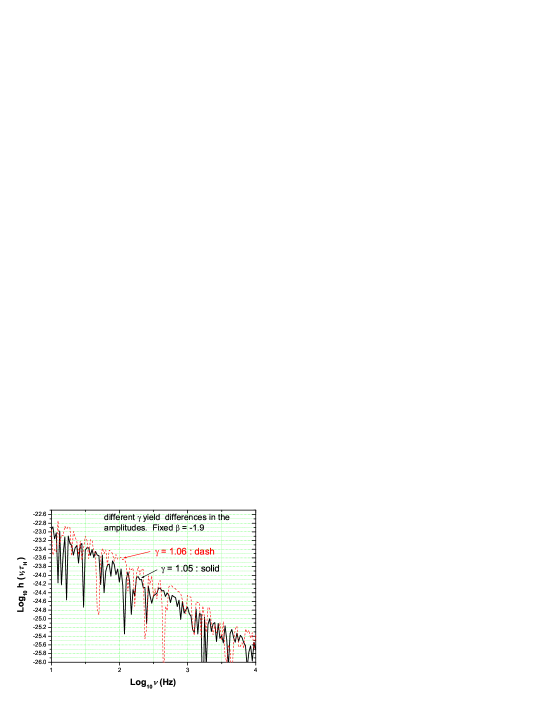
Figure 12: For a fixed $\beta=-1.9$ this enlarged picture in the range $\nu=10-10^{4}$Hz shows fine differences in the spectrum $h(\nu,\tau_{H})$ for different acceleration models. Again the amplitude of $h(\nu,\tau_{H})$ for the model $\gamma=1.06$ is about $\sim 50\%$ higher than that of model $\gamma=1.05$. Now in the range $\nu=10^{2}-3\times 10^{2}$Hz the amplitude is about $\sim 10^{-24}$, accessible to the LIGO as it approaches its designed sensitivity $10^{-24}$.

Let us examine the dependence of the spectrum $h(\nu,\tau_{H})$ upon the dark energy $\Omega_{\Lambda}$ through the acceleration model parameter $\gamma$. In Fig.10 for a fixed $\beta=-2.0$ we plot two spectra $h(\nu,\tau_{H})$ for the acceleration models $\gamma=1.05$ and $\gamma=1.06$ in a broad range of frequencies. As is seen, the difference between these two acceleration models are small. To show the details in the enlarged pictures, in Fig.12 and Fig.11 we have plotted the spectra in a narrow range of frequencies. It can be read that the amplitude of the model $\gamma=1.06$ is about $\sim 50\%$ greater than that of the model $\gamma=1.05$. That is, in the accelerating Universe with $\Omega_{\Lambda}=0.65$ the amplitude of relic GW is $\sim 50\%$ higher than the one with $\Omega_{\Lambda}=0.7$. Note that the spectrum amplitude $h(\nu,\tau_{H})$ itself is very small, so this amount of $\sim 50\%$ of difference is probably difficult to detect at present. However, in principle, it does provide a new way to tell the dark energy fraction $\Omega_{\Lambda}$ in the Universe. With the LIGO approaching its designed sensitivity, hopefully this difference can be detected thereby. As the LISA is currently designed, it will also be able detect this effect.

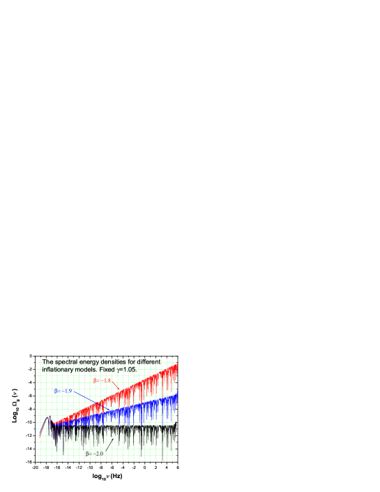
Figure 13: For a fixed $\gamma=1.05$ the spectral energy density $\Omega_{g}(\nu)$ is plotted for the models of $\beta=-1.8$, $\beta=-1.9$, and $\beta=-2.0$. Obviously, the inflationary model of $\beta=-1.8$ has an $\Omega_{g}(\nu)$ increasing too fast with the frequency $\nu$, thus is ruled out by the LIGO bound and the necleosynthesis bound. $\Omega_{g}(\nu)$ in the model of $\beta=-1.9$ is narrowly below the necleosynthesis bound, but since $\Omega_{g}(\nu)$ increases also too fast with $\nu$ so it will barely survive. The model of $\beta=-2.0$ has a flat spectral energy density with a value $\sim 10^{-10}$, much smaller than the necleosynthesis bound. Thus the model $\beta=-2.0$ is robust.

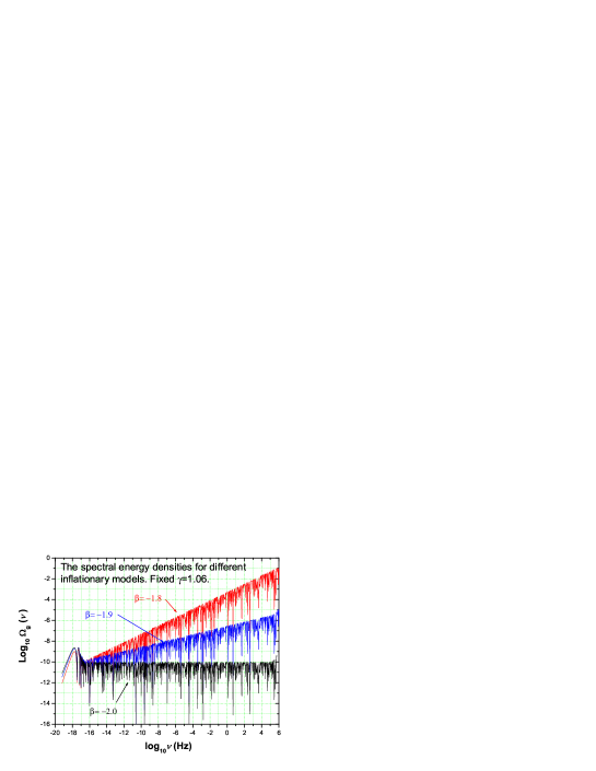
Figure 14: This picture is similar to Fig.13 but for a fixed $\gamma=1.06$. The conclusions are also similar to Fig.13.

Let us examine the spectral energy density $\Omega_{g}(\nu)$ and their constraints. Fig.13 and Fig.14 are the plots of the spectral energy density $\Omega_{g}(\nu)$ defined in Eq.(17) for $\gamma=1.05$ and $\gamma=1.06$, respectively. These plots of the exact analytic results agree with the numerical one in zh2 . If we use the result LIGO third science run b-abbott1 of the energy density bound for the flat spectrum with $\Omega_{0}<8.4\times 10^{-4}$ in the $69-156$ Hz band, then the model $\beta=-1.8$ is ruled out, but the models $\beta\leq-1.9$ survive. However, this LIGO constraint on the GW energy density is not as stringent as the constraint by the so-called nucleosynthesis bound maggiore maia2 , whose main idea is the following: In the early Universe at a temperature $T\sim$ a few Mev the nucleosynthesis process is going on. The relic GW will contribute to the total energy density $\rho$ that drives the Universe expansion, thus will increase the effective number of species of particles $g_{*}$. More relic GW energy will enhance the freeze-out temperature for the process $pe\leftrightarrow n\nu$, and will lead to more neutrons available for the production of helium-4 (${}^{4}He$). In practice the effective number of neutrino species $N_{\nu}$ is used in place of $g_{*}$. Analysis has led to the nucleosynthesis bound on the relic GW energy density at the present time maggiore :

$$\int\Omega_{g}(\nu)\,d(\log\nu)\leq 0.56\times 10^{-5}.$$ (41)

where the value $\rho_{\gamma}\simeq 2.481\times 10^{-5}\rho_{c}$ and the conservative value $N_{\nu}<4$ have been used. Note that this is bound on the total GW energy density integrated over all frequencies. The integrand function should also have a bound $\Omega_{g}(\nu)<0.56\times 10^{-5}$ in the interval of frequencies $\delta(\log\nu)\simeq 1$. By this constraint it is also seen from Fig.13 and Fig.14 that the model $\beta=-1.8$ has an $\Omega_{g}(\nu)$ too high, is therefore ruled out, the same conclusion that we arrived at from Fig.6 and Fig.7. The model with $\beta=-1.9$ are barely alive, as its energy density $\Omega_{g}(\nu)$ tends to be growing higher with high frequencies. The model $\beta=-2.0$ are still robust since its spectral energy density $\Omega_{g}(\nu)$ is a flat function much lower than the limit in Eq.(41).

VI Analytic Approximation

We now want to give an approximation to the above exact solution $h(k,\tau_{H})$ to recover the approximate analytic one given in zh . The following approximation for the Bessel functions will be used

$$J_{\mu}(x)\approx\sqrt{\frac{2}{\pi x}}\cos(x-\frac{\mu\pi}{2}-\frac{\pi}{4}),\,\,\,\,\,x\gg 1,$$ (42)

$$J_{\mu}(x)\approx\frac{1}{\Gamma(\mu+1)}(\frac{x}{2})^{\mu},\,\,\,\,\,x\ll 1.$$ (43)

Note that the coefficients $D_{1},D_{2}$, $B_{1}$, $B_{2}$, $C_{1}$, $C_{2}$, $E_{1}$, and $E_{2}$ are all functions of $k$, and they need to be approximated according to the value of $k$.

In the long-wave limit, $\ x_{1}=k\tau_{1}\ll 1$ and $t_{1}=(1+\beta_{s})x_{1}/(1+\beta)\ll 1$, from Eqs.(V) and (V) one has

$$D_{1}\approx 2^{-\beta+\beta_{s}}(\frac{1+\beta}{1+\beta_{s}})^{\beta+1}t_{1}^{\beta-\beta_{s}}A_{1},\,\,\,\,\,\,\,D_{2}\approx t_{1}^{\beta+\beta_{s}+3}A_{1}.$$ (44)

$D_{2}$ is higher order of $t_{1}$ and can be neglected in the following.

From Eqs.(31) and (32), in the long-wave limit $t_{s}\ll 1$ and $y_{s}\ll 1$, one has

$$B_{1}\approx it_{s}^{\beta_{s}}D_{1}\propto k^{\beta},\,\,\,\,\,\,\,B_{2}\approx-B_{1}.$$ (45)

From Eqs.(34) and (35) , in the long-wave limit $k\ll 1/\tau_{2}$, one has

$$C_{1}\approx-\frac{3i}{2y_{2}}B_{1}\sim k^{\beta-1},\,\,\,\,\,C_{2}\ll C_{1},$$ (46)

so $C_{2}$ can be neglected. In the shortwave limit $k\gg 1/\tau_{2}$, one has

$$C_{1}\approx-2iB_{1}\sin z_{2},\,\,\,\,\,C_{2}\approx 2iB_{1}\cos z_{2}.$$ (47)

From Eqs.(V) and (V), for $k\tau_{E}\ll 1$, one has

$$E_{1}\approx C_{1},\,\,\,\,\,E_{2}\approx C_{2},$$ (48)

which also holds approximately for $k\tau_{E}\gg 1$, with some extra oscillating factors.

With all these coefficients being estimated, now we can evaluate the approximation of the spectrum in Eq.(15) at the present time $\tau_{H}$, which is written as

$$h(k,\tau_{H})=A\frac{l_{0}}{2\pi b}k|\frac{\mu_{k}(\tau_{H})}{a(\tau_{H})}|.$$

Substituting the expressions Eq.(36) for $\mu_{k}(\tau_{H})$ and Eq.(9) for $l_{0}$ into the above leads to

$$h(k,\tau_{H})=A[\gamma(\zeta_{E}^{-(1+\frac{1+\beta}{\gamma})}\zeta_{2}^{\frac{\beta-1}{2}}\zeta_{s}^{\beta}\zeta_{1}^{\frac{\beta_{s}-\beta}{1+\beta_{s}}}]\frac{k}{k_{H}}\sqrt{\frac{\pi s_{H}}{2}}|E_{1}J_{\gamma+\frac{1}{2}}(s_{H})+E_{2}J_{-\gamma-\frac{1}{2}}(s_{H})|.$$ (49)

Using the results from Eq.(42) through Eq.(48), we approximate this expression by the leading term of power-law of $k$ in various ranges of $k$. By some straightforward calculations, using $|(\tau_{H}-\tau_{a})/(\tau_{E}-\tau_{2})|=1/(1+z_{E})$, we obtain the following expressions for the analytic approximate spectrum

$$h(k,\tau_{H})=A(\frac{k}{k_{H}})^{2+\beta},\,\,\,\,\,k\leq k_{E};$$ (50)

$$h(k,\tau_{H})\approx A(\frac{k}{k_{H}})^{\beta-1}\frac{1}{(1+z_{E})^{3+\epsilon}},\,\,\,\,\,k_{E}\leq k\leq k_{H};$$ (51)

$$h(k,\tau_{H})\approx A(\frac{k}{k_{H}})^{\beta}\frac{1}{(1+z_{E})^{3+\epsilon}},\,\,\,\,\,k_{H}\leq k\leq k_{2};$$ (52)

$$h(k,\tau_{H})\approx A(\frac{k}{k_{H}})^{\beta+1}\frac{k_{H}}{k_{2}}\frac{1}{(1+z_{E})^{3+\epsilon}},\,\,\,\,\,\,\,k_{2}\leq k\leq k_{s};$$ (53)

$$h(k,\tau_{H})\approx A(\frac{k_{s}}{k_{H}})^{\beta_{s}}\frac{k_{H}}{k_{2}}(\frac{k}{k_{H}})^{\beta-\beta_{s}+1}\frac{1}{(1+z_{E})^{3+\epsilon}},\,\,\,\,\,\,\,k_{s}\leq k\leq k_{1},$$ (54)

where the small parameter $\epsilon\equiv(1+\beta)(1-\gamma)/\gamma$, also depending on the behavior of the acceleration expansion through $\gamma$. The model $\gamma=1$ gives $\epsilon=0$, and the results of Eqs.(50) through (54) reduce to exactly our early result given in zh . The influence of detailed accelerating expansion on the $h(k,\tau_{H})$ is mainly demonstrated through the factor $1/(1+z_{E})^{3+\epsilon}$, causing a variation in the magnitude of $h(k,\tau_{H})$. For the inflationary expansion with $\beta\approx-2$ , the model of $\gamma=1.05$ ($\Omega_{\Lambda}=0.7$) gives $1/(1+z_{E})^{3+\epsilon}=0.423$, and the model $\gamma=1.06$ ($\Omega_{\Lambda}=0.65$) gives $1/(1+z_{E})^{3+\epsilon}=0.533$, yielding roughly the amplitude of the model $\gamma=1.06$ greater than that of the $\gamma=1.05$ by about $\sim 30\%$. The more accurate computation from the exact solutions shows an average difference of $\sim 50\%$, as plotted in Figs.(12) and (11). Note that the factor $1/(1+z_{E})^{\epsilon}=0.987$ for the model $\gamma=1.05$, and $1/(1+z_{E})^{\epsilon}=0.989$ for the model $\gamma=1.06$, differing by only $0.2\%$, too small to tell by the current experimental detections. Therefore, in regards to the amplitude of relic GW, one can simply put $\epsilon=0$ in the approximate spectrum given in Eqs.(50) through (54), just as it was in the model $\gamma=1$, causing only a difference of $0.2\%$ in the amplitude for a variety of models with various $\gamma$.

We remark that each of these expressions from Eq.(51) to (54) holds up to a numerical factor $A$, which contains certain oscillating factors of the form $\cos(k\tau_{H})$, or $\cos(y_{2})$ and $\sin(t_{s})$. In comparison with the decelerating models grishchuk , Eq.(51) is a new segment of spectrum in $k_{E}<k<k_{H}$, whose occurrence is due to the acceleration of current expansion of the Universe. Besides, the three segments of spectrum, i.e., Eqs .(52), (53), and (54), all have the extra factor $(1+z_{E})^{-3-\epsilon}=(\Omega_{m}/\Omega_{\Lambda})^{1+\epsilon/3}$ that are missing in the corresponding three segments in the decelerating models.

VII Conclusion

We have presented a detailed calculation of the exact analytic spectrum of relic GW in the present flat $\Omega_{\Lambda}+\Omega_{m}=1$ Universe in accelerating expansion. The resulting exact spectrum explicitly depends on the detailed behavior of the present accelerating expansion, characterized by the parameter $\gamma$ in the scale factor $a(\tau)\propto|\tau|^{-\gamma}$. It also explicitly depends on the inflationary model $\beta$, the reheating model $\beta_{s}$, and the (tensor/scalar) ratio $r$ as well. Therefore, the result is general enough to describe the GW spectrum $h(\nu,\tau_{H})$ produced from in a variety of accelerating cosmological models. One can use the formula in other applications by choosing a set of parameters $\beta$, $\beta_{s}$, $\gamma$, and $r$. Besides, the analysis of the exact result gives the following conclusions:

The GW amplitude of the model $\gamma=1.06$ is about $\sim 50\%$ greater than that of the model $\gamma=1.05$, i.e., in the accelerating Universe with $\Omega_{\Lambda}=0.65$ the amplitude of relic GW is $\sim 50\%$ higher than the one with $\Omega_{\Lambda}=0.7$. Although it is probably difficult to detect at present, the effect does provide a new way to tell the dark energy fraction $\Omega_{\Lambda}$ in the Universe. Hopefully this difference can be detected when the LIGO approaches its designed sensitivity $\sim 10^{-24}$, and the LISA runs in future.

The spectrum depends sensitively on the parameter $\beta$ of the inflationary models. A larger value of $\beta$ yields a flatter spectrum $h(\nu,\tau_{H})$ with more power on the higher frequencies. The sensitivity curve of current LIGO rules out the inflationary models with $\beta\geq-1.8$. The LIGO with its design sensitivity and the LISA in future will also be able to test the $\beta=-1.9$ model directly.

The relic GW is also constrained through its spectral energy density $\Omega_{g}(\nu)$ by the resent LIGO bound and the nucleosynthesis bound. While both bounds rule out the inflationary model $\beta=-1.8$, the nucleosynthesis bound puts the model $\beta=-1.9$ in danger. However, the model $\beta=-2.0$ (de Sitter) is robust, since its spectral energy density $\Omega_{g}(\nu)$ is flat and is $\sim 10^{-10}$, much smaller than the nucleosynthesis bound.

Finally, the exact analytic spectrum reduces to the approximate analytic and the numerical ones given in our previous study for the case $\gamma=1$.

References

- (1) R.Abbott, et. al. Phys.Rev. D72 (2005) 062001, gr-qc/0505029.
- (2) R. Abbott, Phys.Rev.Lett. 94, 181103 (2005).
- (3) B. Abbott, et. al. Phys.Rev.Lett. 95 (2005) 221101, gr-qc/0507254.
- (4) B. Abbott, et. al. Phys.Rev. D72 (2005) 102004, gr-qc/0508065.
- (5) A.A.Starobinsky, JEPT Lett. 30, 682 (1979).
- (6) V.A. Rubakov, M.V.Sazhin, and A.V.Veryaskin, Phys.Lett.115B, 189 (1982).
- (7) L.F.Abbott and D.D.Harari, Nucl.Phys. B264, 487 (1986).
- (8) B.Allen, Phys.Rev.D37, 2078 (1988).
- (9) V.Sahni, Phys.Rev.D42, 453 (1990).
- (10) L.Grishchuk, Class.Quant.Grav. 14 1445 (1997); Lecture Notes Physics 562, 164 (2001), in “Gyros, Clocks, Interferometers…: Testing Relativistic Gravity in Space”, Lammerzahl, et. al. (Eds).
- (11) M.R.G. Maia and J.D. Barrow, Phys.Rev.D50, 6262 (1994).
- (12) A. Riszuelo and J-P Uzan, Phys.Rev.D62, 083506, (2000).
- (13) H. Tashiro, K. Chiba, and M. Sasaki, Class.Quant.Grav. 21 1761 (2004).
- (14) A.B. Henriques, Class.Quant.Grav. 21, 3057 (2004); A.B. Henriques and L.M.Mendes, Phys.Rev.D52 2083 (1995).
- (15) G. Gong, Class.Quant.Grav. 21 (2004) 5555-5562.
- (16) C. Ungarelli, et. al. Class.Quant.Grav. 22 S955-S964 (2005).
- (17) T. L. Smith, M. Kamionkowski, and A. Cooray, astro-ph/0506422.
- (18) L.B. Boyle and P.J. Steinhardt, astro-ph/0512014 .
- (19) A. Cooray, et. al. Phys.Rev. D72 023514 (2005).
- (20) W.Hu and M. White, Phys.Rev.D56 (1997) 597.
- (21) M.Zaldarriaga and D.D.Harari, Phys.Rev. D52 (1995) 3276; D.Harari and M.Zaldarriaga, Phys.Lett.B310 (1993) 96;
- (22) M.Kamionkowski, A.Kosowsky, A.Stebbins, Phys.Rev. D55 (1997) 7368.
- (23) B.Keating, et al, Astrophys.J. 495 (1998) 580.
- (24) Y.Zhang, H.Hao and W.Zhao, Acta.Astron.Sinica 46 (2005) 1.
- (25) L.Grishchuk, Uspekhi Fiz. Nauk v.176 (2006), gr-qc/0504018.
- (26) A. Riess, et al., AJ 116, 1009 (1998).
- (27) S.Perlmutter, et al., Astrophys.J.517, 565 (1999).
- (28) N.A. Bahcall, J.P.Ostriker, S.Perlmutter, P.J.Steinhardt, Science 284, 1481 (1999).
- (29) D.N.Spergel, et al., Astrophys.J. Suppl. 148, 175 (2003).
- (30) Y. Zhang, Gen.Rel.Grav. 34, 2155 (2002); Gen.Rel.Grav. 35, 689 (2003).
- (31) J.C. Fbris, S.V.B. Goncalves, and M.S. Santos, Gen. Rel. Grav.36 2559 (2004).
- (32) M.S. Santos, Proc. of the Conference on Magnetic Fields in the Universe: from laboratories and stars to primordial structures, AIP(NY), eds. E. M. de Gouveia Dal Pino, G. Lugones and A. Lazarian (2005). gr-qc/0504032.
- (33) Y. Zhang, et. al., Class.Quant.Grav. 22, 1383 (2005).
- (34) Y. Zhang and W. Zhao, Chin.Phys.Lett. 22, 1817 (2005).
- (35) L.Grishchuk, Sov.Phys.JETP, Vol. 40, No.3, 409 (1974).
- (36) Ya. B. Zel’dovich and I.D. Novikov, The Structure and Evolution of the Universe, The University of Chicago Press, (1983), Vol.2.
- (37) L. Parker, Phys.Rev. 183 (1969) 1057.
- (38) H.V.Peiris, et al. Astrophys.J.Suppl. 148 (2003) 213.
- (39) U.Seljak et al., Phys.Rev.D71 (2005) 103515.
- (40) L.Parker, ”The production of elementary particles by strong gravitational fields” in “Asymptotic Structure of Space-Time”, eds. S.Deser and M.Levy (New York: Plenum) (1979).
- (41) N.D. Bunch and P.C.W. Davies, “Quantum Fields in Curved Space”, Cambridge University Press (1982).
- (42) LISA sensitivity curve can be obtained from — http://www.srl.caltech.edu/ shane/sensitivity/
- (43) M. Maggiore, Phys. Rept. 331 (2000), 283.
- (44) M.R. G. Maia, Phys.Rev.D48, 647 (1993).