Confronting quintessence models with recent high-redshift supernovae data

Abstract

We confront the predictions of different quintessence models with recent measurements of the luminosity distance from two sets of supernovae type Ia. In particular, we consider the 157 SNe Ia in the Gold dataset with $z<1.7$, and the more recent data containing 71 supernovae obtained by the Supernova Legacy Survey (SNLS) with $z<1$. We numerically solve the evolution equations for the Ratra-Peebles inverse power law model, the double exponential and the hyperbolic cosine quintessence models. We obtain confidence regions from the two datasets in the $\Omega_{M}-\alpha$ and $\Omega_{M}-w_{\phi}$ planes for the different models and compare their predictions with dark energy models with constant equation of state.

I Introduction

The growing observational evidence from high-redshift supernovae Gold ; SNLS and other cosmological data WMAP suggests that the dominant component of the universe today is some sort of dark energy fluid with negative pressure review ; review2 . Indeed a component with constant equation of state $p_{X}=w_{X}\rho_{X}$ and $w_{X}<-0.78$ WMAP fits the existing data with reasonable goodness (XCDM model). In particular, it includes the most economical explanation for the present state of accelerated expansion of the universe, i.e., the presence of a pure cosmological constant with $w_{X}=-1$. However, ther are other models in which the equation of state depends on redshift and which are also able to fit the data with comparable quality. This is the case of the so called quintessence models RP ; quintessence , in which it is the presence of an evolving scalar field with appropriate potential term what plays the role of dark energy.

Quintessence models exhibit an interesting property usually called tracking behaviour tracking . This means that there is a wide range of initial conditions for which the evolution of the scalar fields converges to a common evolutionary track. Furthermore in such a tracking regime the equation of state of quintessence $w_{\phi}$ remains almost constant. Moreover there are particular models, usually called scaling models scaling ; scaling2 ; scaling3 , in which $w_{\phi}$ mimics the equation of state of the dominant component throughout the cosmological evolution. These properties allow quintessence models to alleviate the fine tuning problem of XCDM models, although in any case the scale of the quintessence potential has always to be tuned in order to reproduce the data.

Apart from quintessence, other models have been proposed in the literature. Thus for instance, scalar fields with non-canonical kinetic terms (k-essence) k-essence ; the generalized Chaplygin gas model Chaplygin , which in principle allows for an unification of dark energy and dark matter; infrared modifications of General Relativity, as for instance in extra dimensional theories infrared or the modification of the Friedmann equation in the so called Cardassian models Cardassian ; Bento .

The present SNe Ia data are not very constraining when trying to determine the nature of dark energy and different dataset favor different regions of the parameter space. Thus for instance, it is known that the Gold dataset Gold prefers models with $w_{X}<-1$ ness1 ; pref_phantom , the so called phantom dark energy models, whereas for the more recent Supernova Legacy Survey (SNLS) SNLS , the best fit is closer to a pure cosmological constant Nesseris ; pref_LCDM . Therefore it is worth exploring what kind of constraints are imposed in each case, and this is the aim of the present work. However the information we will obtain will be very limited because even the highest redshift points in those sets explore only relatively recent epochs, and therefore the present supernovae data alone are not able to discriminate between the different models (although larger future supernovae catalogues are expected to improve in an important way the present constraints). Accordingly we should rely on complementary information in order to distinguish quintessence models from a cosmological constant or other alternatives alter1 ; alter . Thus for instance, in the particular case of quintessence, dark energy is generated by a scalar field, and there exists the possibility of having density or velocity perturbations which could affect CMB anisotropies DEperturbations . In constrast, the pure cosmological constant case does not support such perturbations.

In this work we will concentrate on different quintessence models and derive constraints on their parameters from the two mentioned Gold and SNLS datasets. We consider three models: an inverse power-law Ratra-Peebles (RP) model RP , $V(\phi)=M^{4+\alpha}/\phi^{\alpha}$, the double exponential (DE) potential $V(\phi)=M^{4}(e^{\alpha\phi}+e^{\beta\phi})$ DE ; DE2 which exhibits scaling behaviour and the hyperbolic cosine (HC) $V(\phi)=M^{4}(\cosh(\lambda\phi)-1)^{\alpha}$ HC , which posseses an oscillatory behaviour at recent epochs. Unlike previous works param_w ; ichikawa , we do not parametrize the equation of state $w_{\phi}(z)$ in order to obtain explicit expressions for the luminosity distance-redshift relation $d_{L}(z)$. Instead, we solve numerically the evolution equation for the scalar field and the universe scale factor. This allows us to numerically obtain $d_{L}(z)$ for each model. The value of the fitted cosmological parameters is known to have a strong dependence on the particular parametrization chosen for the equation of state (see bassett ; review2 and references therein). In particular, at least three parameters are needed in order to take into account properly all the information encoded in the SNIa data. Our approach does not rely on particular parametrizations, but instead we consider the full redshift dependence by numerically solving the evolution equations.

The plan of the paper goes as follows, in section 2 we review the models properties and obtain the appropriate equations of motion. In section 3, we compute the luminosity distance expressions and perform the corresponding cosmological fits. Section 4 contains the main results of the paper with the confidence regions for different spaces of parameters and finally we include a brief section with conclusions.

II Quintessence models and evolution equations

II.1 Inverse power law potential

In the first model that we will consider, the potential reads:

$$V(\phi)=\frac{M^{4+\alpha}}{\phi^{\alpha}}$$ (1)

This model has a tracker attractor, but it is not scaling, although the equation of state is determined by that of the dominant component:

$$w_{\phi}=\frac{\alpha w_{R,M}-2}{\alpha+2}$$ (2)

where, for $\alpha>-2$, in the radiation or matter eras we have $w_{\phi}<w_{R,M}$ respectively, i.e. the energy density decreases more slowly than the dominant component and it eventually becomes dominant at late times. The corresponding equations of motion reduce to the Friedmann equation for the scale factor, together with the scalar field evolution equation:

$$H^{2} = \frac{8\pi G}{3}\left(\frac{\dot{\phi}^{2}}{2}+V(\phi)+\sum_{i=M,R}\rho_{i,0}a^{-3(w_{i}+1)}\right)$$

$$\ddot{\phi} + 3H\dot{\phi}+V^{\prime}(\phi)=0$$ (3)

where $\rho_{i,0}/\rho_{0}=\Omega_{i}$ with $i=M,R$ and $\rho_{0}$ is the critical density. Here a dot denotes derivative with respect to cosmological time.

In order to solve these equations numerically, we transform them into dimensionless equations, defining: $\tau=H_{0}t$ and $\tilde{\phi}=(8\pi G)^{1/2}\phi$. Now a prime will denote derivative with respect to $\tau$:

$$\frac{\tilde{\phi}^{\prime\prime}}{3} + \tilde{\phi}^{\prime}\frac{a^{\prime}}{a}+\tilde{V}^{\prime}(\tilde{\phi})=0$$

$$\left(\frac{a^{\prime}}{a}\right)^{2} = \frac{\tilde{\phi}^{\prime 2}}{6}+\tilde{V}(\tilde{\phi})+\Omega_{R}a^{-4}+\Omega_{M}a^{-3}$$ (4)

where

$$\tilde{V}(\tilde{\phi}) = \frac{A}{\tilde{\phi}^{\alpha}}$$

$$A = \frac{M^{4+\alpha}(\sqrt{8\pi G})^{\alpha+2}}{3H_{0}^{2}}$$ (5)

The initial conditions for $\tilde{\phi}$ and $a$ will be given by: $\tilde{\phi}(0)=5\cdot 10^{-1}$, $\tilde{\phi}^{\prime}(0)=0$ and $a(0)=10^{-3}$. We will explore the parameters range $\alpha=0-5.5$ and $A=0.3-8\cdot 10^{4}$. Notice that for those values of the parameters, the initial scalar field energy density is a small fraction of $\rho_{M}$ and $\rho_{R}$. Notice also that thanks to the attractor behaviour, the late time evolution is not very sensitive to the particular initial conditions chosen.

II.2 Double exponential potential

In this case:

$$V(\phi)=M^{4}(e^{\alpha\kappa\phi}+e^{\beta\kappa\phi})$$ (6)

where $\kappa=\sqrt{8\pi G}$. The energy density in this model follows a scaling behaviour at early time, whereas it becomes dominant at late times with appropriate equation of state: $w_{\phi}\simeq-1$. The corresponding dimensionless potential now reads:

$$\tilde{V}(\tilde{\phi}) = A(e^{\alpha\tilde{\phi}}+e^{\beta\tilde{\phi}})$$

$$A = \frac{M^{4}(8\pi G)}{3H_{0}^{2}}$$ (7)

and the corresponding equations of motion are given in (4). The initial conditions are $\tilde{\phi}(0)=0.5$, $\tilde{\phi}^{\prime}(0)=0$ and $a(0)=10^{-3}$. The range of parameters considered are $\beta=20$, $\alpha=0.1-1.5$ and $A=0.4-120$, where for simplicity we have fixed the constant $\beta$. The $\alpha$ and $\beta$ constants essentially fix the value of $w_{\phi}$ today, and we have checked that fixing $\beta$ still allows us to cover a wide range of values in $w_{\phi}$, just varying $\alpha$. Again for those particular values, the initial energy density in the scalar field is a small fraction of the radiation and matter densities.

II.3 Hyperbolic cosine potential

In this case the dimensionless potential reads:

$$\tilde{V}(\tilde{\phi}) = A(\cosh(\lambda\tilde{\phi})-1)^{\alpha}$$

$$A = \frac{M^{4}(8\pi G)}{3H_{0}^{2}}$$ (8)

In the limit $\lambda\tilde{\phi}\gg 1$, i.e. at early times, the potential behaves as a single exponential and it is possible to choose the parameters so that the model posseses a scaling behaviour. In the opposite limit, $\lambda\tilde{\phi}\ll 1$ (late times), the potential can be approximated by $\tilde{V}(\tilde{\phi})\propto(\lambda\tilde{\phi})^{2\alpha}$, and the scalar field oscillates around $\tilde{\phi}=0$. When oscillations start, the equation of state no longer mimics the dominant component, but it also start oscillating with average value given by:

$$\langle w_{\phi}\rangle=\frac{\alpha-1}{\alpha+1}$$ (9)

Accordingly, the value of $\alpha$ determines the present equation of state. For $\alpha=1$ the oscillations behaves as nonrelativistic matter, whereas if we require accelerated expansion today, i.e. $w_{\phi}<-1/3$ then we should have $\alpha<1/2$.

The numerical integration of equations (4) now has an additional difficulty. In the interesting case ($\alpha<1/2$), the potential derivative $\tilde{V}^{\prime}$ appearing in the first equation diverges at the origin. Since both $\tilde{\phi}$ and $\tilde{\phi}^{\prime}$ are continuous at the origin, in order to avoid numerical instabilities we have smoothed the divergence modifiying the potential as $V(\tilde{\phi})=A(\cosh(\lambda\tilde{\phi})-(1-\epsilon))^{\alpha}$. We have checked that for sufficiently small values, the results do not depend on the $\epsilon$ parameter.

The initial conditions considered are $\tilde{\phi}(0)=1.6$, $\tilde{\phi}^{\prime}(0)=0$, $a(0)=10^{-3}$. The free parameters are $\alpha=0.02-0.4$, $A=0.3-14$ and we have fixed $\lambda\alpha=5$, which ensures again that initially quintessence is not the dominant component of the energy density and that it follows a scaling behaviour.

III Cosmological data fit

After numerically solving (4), we obtain a discrete time evolution for the scale factor $a(t)$ and the scalar field $\phi(t)$ for a given set of parameters $(A,\alpha)$. The time dependence will be used to compute the theoretical values of the luminosity distance to each SNe Ia with a given redshift z. Thus we use the well known expression, derived from the FRW metric under flat prior, expressed in terms of the dimensionless time variable $\tau$.

$$d_{L}(\tau)=\frac{a(\tau_{0})}{a(\tau_{1})}\int_{\tau_{0}}^{\tau_{1}}\frac{d\tau}{a(\tau)}$$ (10)

The observations of supernovae measure essentially the distance modulus $\mu$, which is the diference between the apparent magnitude m and the absolute magnitude M, and relates to the luminosity distance as:

$$\mu_{th}=m-M = 5\log{d_{L}}+5\log\left(\frac{cH_{0}^{-1}}{\mbox{Mpc}}\right)+25$$ (11)

$$= 5\log{d_{L}}+\tilde{M}$$

The $M$ value can be assumed constant once the necessary corrections are applied on $m(z)$.

Assuming $\tau_{0}$ to be the value for which $a(\tau_{0})=1$, the scale factor depends on redshift as $a(\tau)=(z+1)^{-1}$. As a consequence, for each supernovae in a given set, we derive $a(\tau_{1})$ from its redshift and obtain $\tau_{1}$ from the numerical output data of (4). Hence the integral (10) can be numerically evaluated to obtain $\mu_{th}$ for each ($A$, $\alpha$), once the value of $H_{0}$ is fixed.

Once we obtain $\mu_{th}$, the comparison to its observational value will enable us to carry out a $\chi^{2}$ statistical analysis. For this purpose, we have considered two sets of supernovae. On one hand, the Gold set, compiled by Riess et. al. Gold , containing 143 points from previously published data, plus 14 points with $z>1$ discovered with the HST, all reduced under the same criteria in order to improve the errors arising from systematics. On the other, the SNLS set, comprising 71 distant supernovae ($0.15<z<1$) discovered during the first year of the Supernova Legacy Project (SNLS) SNLS , alongside with 44 SNe Ia from other sources that feeds the nearby zone ($0.0015<z<0.125$), and which are also included in the Gold set.

The process followed to obtain $\chi^{2}$ is slightly different for each set. In the Gold set we have used the observational distance modulus $\mu_{exp}$ given by Riess et. al. together with its associated error $\sigma_{\mu}$ to compute $\chi^{2}$ as a function of the free parameters of the quintessence model.

$$\chi^{2}(A,\alpha,\tilde{M})=\sum_{i=1}^{N}\frac{(\mu_{obs}-\mu_{th}(A,\alpha,\tilde{M}))^{2}}{\sigma_{i\mu}^{2}}$$ (12)

The dependence on $H_{0}$ has been accounted for in (12) through the nuissance parameter $\tilde{M}$, which is independent of the data points and the data set. We have marginalized $\chi^{2}$ over all values of $\tilde{M}$ by expanding and minimizing (12) with respect to $\tilde{M}$ (see Bento ; Nesseris ; ness1 ).

On the other hand, for the SNLS data, a more detailed relation between $\mu$ and the observational measurements has to be considered in the statistical analysis, which implies recursively fitting two new non-cosmological parameters in the calculation of $\chi^{2}$.

The expression for the observational distance modulus used by the SNLS team includes these two parameters to measure the impact of the rest frame color parameter ($c$), and the light curve strecht ($s$), on the distance modulus.

$$\mu^{SNLS}_{obs}=m(z)-M+a_{1}(s-1)-a_{2}c$$ (13)

Introducing this equation into the expression for $\chi^{2}$

$$\chi^{2}(\alpha,A,a_{1},a_{2},M+\tilde{M})=$$

$$\sum_{i=1}^{N} \frac{(\mu_{obs}^{SNLS}(a_{1},a_{2},M)-\mu_{th}(A,\alpha,H_{0},\tilde{M}))^{2}}{\sigma_{i\mu}^{2}}$$

we obtain a six parameter dependence (five parameters in practice, since we can replace $M+\tilde{M}$ by a single additive constant) We minimize following the process suggested in SNLS , i.e. marginalizing with respect to $a_{1}$, $a_{2}$ and $M+\tilde{M}$ for each pair of $(A,\alpha)$ values. Notice that marginalizing over $M$ or $M+\tilde{M}$ is equivalent to marginalize with respect to $H_{0}$. Again $\mu$ and $\sigma_{\mu}$ are obtained from the data in SNLS .

IV Results and Model comparison

The best resulting cosmologies obtained after fitting each model to the Gold and SNLS sets are summarized in Table I and II respectively. In each sample, we find the same $\chi^{2}$ for the best fit with the three quintessence models considered in the paper, i.e. $\chi^{2}_{min}=177.0$ for the 157 SNe Ia of the Gold set, and $\chi^{2}_{min}=111.0$ for the 115 SNe Ia of the SNLS set. In addition, the minimun $\chi^{2}$ for all models corresponds to $\alpha=0$. For this value the RP and HC potentials turn into a cosmological constant term and we have used this fact to check our results, finding good agreement for the $\Omega_{M}$ value when compared to the Riess et. al., and Astier et. al. XCDM model. On the other hand, albeit the DE potential does not strictly behave as a $\Lambda$ term, due to the nonvanishing exponential, the $\omega_{\phi}$ value tends asymptotically to -1, leading to the same result as DE and HC. This implies that a quintessence potential, and a pure $\Lambda$CDM model, can not be distinguished only by fitting $(\Omega_{M},\omega_{\phi})$, since a quintessence model can be tuned to accurately resemble a cosmological constant, at least in the redshift interval explored by the actual SNe Ia sets. In any case, notice that $\rho_{\phi}$ evolves in time for any non-zero value of $\alpha$ for the three potentials.

	Gold
	$\Omega_{M}$	$\omega_{\phi}$	$\alpha$	$\chi^{2}$
RP	0.30$\pm^{0.06}_{0.11}$	-1$\pm^{0.24}_{\;-}$	0$\pm^{1.20}_{\;-}$	177.0
HC	0.30$\pm^{0.06}_{0.10}$	-1$\pm^{0.24}_{\;-}$	0$\pm^{1.35}_{\;-}$	177.0
DE	0.30$\pm^{0.06}_{0.07}$	-1$\pm^{0.22}_{\;-}$	0$\pm^{1.08}_{\;-}$	177.0

Table 1: Best fitting cosmological parameters, with their associated $68\%$ errors for the Gold set. The degeneracy in $\alpha=0$ leads to the same value of $\Omega_{M}$ for the three potentials in a set. Moreover, due to the form of the quintessence Lagrangian values of $\omega_{\phi}$ below -1 cannot be obtained.

Combining the data obtained by solving (4) for each potential, we may relate ($A,\alpha$), and its corresponding fitting $\chi^{2}$, to a single ($\omega_{\phi},\Omega_{M}$) pair which allows us to plot the confidence regions for the two parameter combinations $(\alpha,\Omega_{M})$ and $(\omega_{\phi},\Omega_{M})$.

For the HC model, we use directly $\langle\omega_{\phi}\rangle=\frac{1-p}{1+p}$, instead of the value derived from eq.(4), due to the difficulties arising from the calculation of $\langle\omega_{\phi}\rangle^{num}$ in the cases when the oscillations fails to complete a whole period. Moreover, a comparison between $\langle\omega_{\phi}\rangle$ and $\langle\omega_{\phi}\rangle^{num}$ shows a small average discrepancy, $\Delta\omega_{\phi}=10^{-3}$, which justifies our approximation, and serves as a check of the numerical solution.

	SNLS
	$\Omega_{M}$	$\omega_{\phi}$	$\alpha$	$\chi^{2}$
RP	$<$0.36	$<$-0.58	$>$0	111.0
HC	$<$0.36	$<$-0.61	$<$0.3	111.0
DE	$<$0.36	$<$-0.54	$<$1.27	111.0

Table 2: Best fitting cosmological parameters, and upper bounds at $95\%$ C.L. for the SNLS set. The constraints on the cosmological paramaters hold for $\Omega_{M}>0.06$ for the RP and DE potentials, and $\Omega_{M}>0.12$ for the HC.

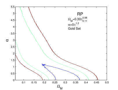
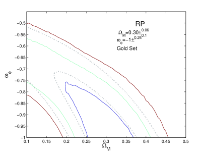
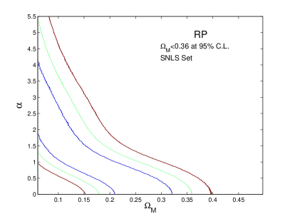
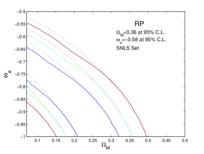
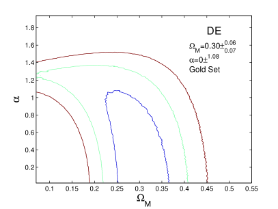
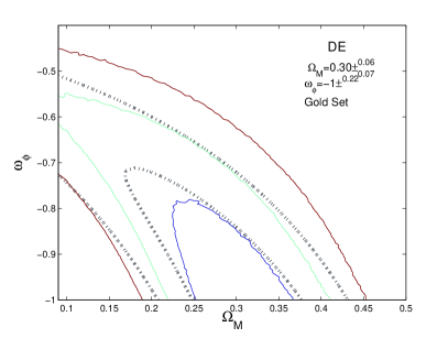
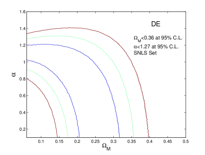
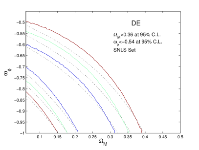
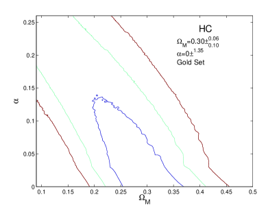
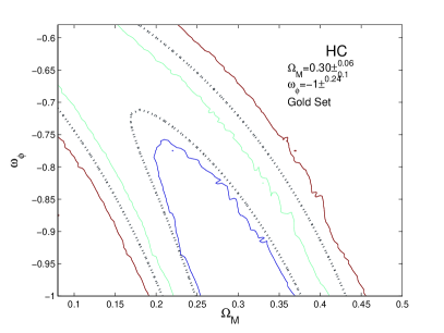
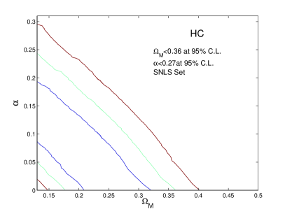
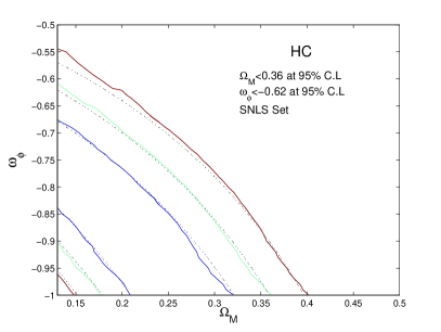
Fig.1 to Fig.3 show the confidence regions for the models in the $\alpha-\Omega_{M}$ and $\omega_{\phi}-\Omega_{M}$ planes, together with the XCDM contour plots. The XCDM regions have been calculated using the same code on the Friedmann equation with a dark energy term ($\rho_{X},\omega_{X}$) instead of a coupled scalar field. In the $\alpha-\Omega_{M}$ plots the contours grow asymptotically for decreasing $\Omega_{M}$ caresia . Nevertheless, as $\omega_{\phi}$ follows the same growing trend, it is possible to restrict the maximum value of $\omega_{\phi}$.

At the $95\%$ confidence level and for $\Omega_{M}>0.1$, we find $\omega^{gold}_{\phi}<$ -0.56, $\omega^{SNLS}_{\phi}<$ -0.58, for the RP model, and $\omega^{gold}_{\phi}<$ -0.55, $\omega^{SNLS}_{\phi}<-0.56$, for the DE model. The HC potential also shows similar results for $\Omega_{M}>0.15$, limiting $\omega^{gold}_{\phi}<$ -0.58, and $\omega^{SNLS}_{\phi}<$ -0.64. Notice that we do not extract any result for values below $\Omega_{M}=$0.1 for RP and DE or $\Omega_{M}=$0.15 for HC, since the computational effort increases in those regions. In fact in the HC model that region is also highly sensitive to the value of the smoothing factor, $\epsilon$.

By comparing the plots for the two datasets, we see that the width of the contours is essentially the same. However, the SNLS $68\%$ C.L. contour never closes for $\Omega_{M}>$0.06, whereas the Gold set constraints the cosmological parameters, for all models, within 0.25$<\Omega_{M}<$0.36 and -1$<\omega_{\phi}<$-0.75, at this significance level. For the RP potential, these results can be compared to analysis done with previous supernovae data in alter1 ; caresia .

Concerning the XCDM contours, one remarkable feature is that as $\omega_{\phi}\mapsto-1$, the SNLS confidence regions for quintessence and XCDM tends to overlap. This is an expected fact, since the best fitting value for XCDM according to Astier et. al., is $\omega_{\phi}=$-1.02, quite close to the quintessence best fit, which is precisely the degenerate case $\alpha=0$. On the other hand, the best fitting value for the Gold set, assuming no priors, is $\omega_{\phi}=$-2.3. This implies an important difference in $\chi^{2}$ with respect to the quintessence models, which prevents the confidence regions from matching. In spite of this, it is noticeable the similarity between contours given the fact that the $68\%$ C.L. region of XCDM is out of the plotted interval. Finally, for all models, the quintessence $99\%$ contours place an outer boundary containing all the XCDM regions, implying that any of the XCDM cosmologies, might be obtained from a quintessence potential.

Figure 1: Confidence regions at the $68\%$, $95\%$ and $99\%$ C.L. (corresponding to $\Delta\chi^{2}$=2.3, 6 and 11.8 for a two-parameter fit) for ($\alpha,\Omega_{M}$) (left panels) and ($\omega_{\phi},\Omega_{M}$) (right panels), in the Ratra-Peebles quintessence potential, obtained using the Gold (top panels) and the SNLS (bottom panels) samples. The dotted lines, on the right panels, show the probability contours for a XCDM model: at the $99\%$ and $95\%$ for the Gold set, and at the $99\%$, $95\%$, and $68\%$ for the SNLS set.

Figure 2: Confidence regions at the $68\%$, $95\%$ and $99\%$ C.L. (corresponding to $\Delta\chi^{2}$=2.3, 6 and 11.8 for a two-parameter fit) for ($\alpha,\Omega_{M}$) (left panels) and ($\omega_{\phi},\Omega_{M}$) (right panels), in the Double Exponential quintessence potential, obtained using the Gold (top panels) and the SNLS (bottom panels) samples. The dotted lines, on the right panels, show the probability contours for a XCDM model: at the $99\%$ and $95\%$ for the Gold set, and at the $99\%$, $95\%$, and $68\%$ for the SNLS set.

Figure 3: Confidence regions at the $68\%$, $95\%$ and $99\%$ C.L. (corresponding to $\Delta\chi^{2}$=2.3, 6 and 11.8 for a two-parameter fit) for ($\alpha,\Omega_{M}$) (left panels) ($\omega_{\phi},\Omega_{M}$) (right panels), in the Hyperbolic Cosine quintessence potential, obtained using the Gold (top panels) and the SNLS (bottom panels) samples. The dotted lines, on the right panels, show the probability contours for a XCDM model: at the $99\%$ and $95\%$ for the Gold set, and at the $99\%$, $95\%$, and $68\%$ for the SNLS set.

V Conclusions

We have compared the predictions of three quintessence models with the measurements of the luminosity distance vs. redshift from two SNe Ia catalogues, (Gold and SNLS surveys). We have obtained the corresponding confidence regions in the ($\alpha,\Omega_{M}$) and ($\omega_{\phi},\Omega_{M}$) planes and compared them with the predictions of dark energy models with constant equation of state (XCDM). From the plots we see that the different confidence regions for quintessence and XCDM models cover essentially the same areas in the ($\Omega_{M},w_{\phi}$) plots. This makes it difficult to discriminate between the different models just from SNe Ia data alone. In all the three cases, the best fit cosmology corresponds to the $\alpha=0$ case, in which the quintessence potential reduces effectively to a cosmological constant. Although SNLS data favor a pure cosmological constant, they yield larger confidence regions than the Gold dataset. Bounds on the cosmological parameters $\Omega_{M}$, $\omega_{\phi}$ and the potential paramaters $\alpha$ have also been obtained. In principle it could be interesting to use the differences in constraints between the two sets as an estimate of possible residual systematics in the SNe Ia data. However, in practice, since both datasets have been obtained and reduced in different ways and possibly the actual data is still dominated by statistical errors, it would be difficult to perform such estimations. In any case this is beyond the scope of the present work.

Acknowledgments: We would like to thank P. Astier for useful comments. This work has been partially supported by DGICYT (Spain) under project numbers FPA 2004-02602 and FPA 2005-02327

References

- (1) A.G. Riess at al. Astrophys.J. 607, 665 (2004)
- (2) P. Astier et al., astro-ph/0510447
- (3) D.N. Spergel et al., Astrophys. J. Suppl. 148, 175 (2003)
- (4) P. J. E. Peebles and B. Ratra, Rev. Mod. Phys. 75, 559 (2003)
- (5) E. J. Copeland, M. Sami and S. Tsujikawa, hep-th/0603057
- (6) B. Ratra and P.J.E. Peebles, Phys. Rev. D37, 3406 (1988)
- (7) C. Wetterich, Nucl. Phys. B302, 668 (1988); R.R. Caldwell, R. Dave and P.J. Steinhardt, Phys. Rev. Lett. 80, 1582 (1998)
- (8) P. J. Steinhardt, L. M. Wang and I. Zlatev, Phys. Rev. D59 123504 (1999)
- (9) E.J Copeland, A.R. Liddle and D. Wands, Phys. Rev. D57, 4686 (1998)
- (10) P. G. Ferreira and M. Joyce, Phys. Rev. D58, 023503 (1998)
- (11) S. Mizuno, S. J. Lee and E. J. Copeland, Phys. Rev. D70, 043525 (2004); E. J. Copeland, S. J. Lee, J. E. Lidsey and S. Mizuno, Phys. Rev. D71, 023526 (2005); M. Sami, N. Savchenko and A. Toporensky, Phys. Rev. D70, 123526 (2004); V. Pettorino, C. Baccigalupi and F. Perrotta, JCAP 0512, 003 (2005); F. Piazza and S. Tsujikawa, JCAP 0407, 004 (2004); S. Tsujikawa and M. Sami, Phys. Lett. B603, 113 (2004)
- (12) C. Armendariz-Picon, T. Damour and V. Mukhanov, Phys. Lett. B458, 209 (1999); T. Chiba, T. Okabe and M. Yamaguchi, Phys. Rev. D62, 023511 (2000)
- (13) A.Y. Kamenshchick, U. Moschella and V. Pasquier, Phys. Lett. B511, 265 (2001); N. Bilic, G.B. Tupper and R.D. Viollier, Phys. Lett. B535, 17 (2002); M.C. Bento, O. Bertolami and A.A. Sen, Phys. Rev. D66, 043507 (2002)
- (14) G. Dvali, G. Gabadadze and M. Porrati, Phys. Lett. B485, 208 (2000); S. Capozziello, S. Carloni and A. Troisi, astro-ph/0303041.
- (15) K. Freese and M. Lewis, Phys. Lett. B540, 1 (2002); S. Sen and A. A. Sen Astrophys.J. 588, 1 (2003)
- (16) M.C. Bento, O. Bertolami, N.M.C. Santos and A.A. Sen, Phys. Rev. D71, 063501 (2005)
- (17) S. Nesseris, L. Perivolaropoulos Phys.Rev. D70 043531 (2004)
- (18) U. Alam, V. Sahni, T. D. Saini, and A. A. Starobinsky, Mon. Not. R. Astron. Soc. 354, 275 (2004); T. R. Choudhury and T. Padmanabhan, Astron. Astrophys. 429, 807 (2005); Y. Wang and P. Mukherjee, Astrophys. J. 606, 654 (2004); D. Huterer and A. Cooray, Phys. Rev. 71, 023506 (2005);
- (19) S.Nesseris, L. Perivolaropoulos, Phys. Rev. D72, 123519 (2005),
- (20) H. K. Jassal, J. S. Bagla, T. Padmanabhan, astro-ph/0601389
- (21) R.R. Caldwell and M. Doran, Phys. Rev. D69, 103517 (2004)
- (22) M. Doran, M.J. Lilley, J. Schwindt and C. Wetterich, Astrophys. J. 559, 501 (2001); M.S. Movahed and S. Rahvar, Phys. Rev. D73, 083518 (2006)
- (23) W. Hu. Astrophys. J. 506, 485 (1998); T. Moroi and T. Takahashi, Phys. Rev. Lett. 92, 091301, (2004); C. Gordon and W. Hu, Phys. Rev. D70, 083003, (2004); A.L. Maroto, JCAP 0605:015 (2006)
- (24) T. Barreiro, E. J. Copeland and N.J. Nunes, Phys. Rev. D61, 127301 (2000)
- (25) A. A. Sen and S. Sheti , Phys.Rev. B532, 159 (2002); I.P. Neupane, Class. Quant. Grav. 21, 4383 (2004); I.P. Neupane, Mod. Phys. Lett. A19, 1093 (2004); L. Jarv, T. Mohaupt and F. Saueressig, JCAP 0408, 016 (2004)
- (26) V. Sahni and L. M. Wang Phys. Rev. D62, 103517 (2000)
- (27) R. Lazkoz, S. Nesseris, L. Perivolaropoulos, JCAP 0511, 010 (2005); V. Barger, E. Guarnaccia, D Marfatia, Phys. Lett. B635, 61-65 (2006)
- (28) K. Ichikawa and T. Takahashi, Phys. Rev. D73, 083526 (2006); Z.K. Guo, N. Ohta and Y.Z. Zhang, Phys. Rev. D72, 023504 (2005)
- (29) B.A. Bassett, P.S. Corasaniti and M. Kunz, Astrophys. J. 617, L1 (2004)
- (30) P. Caresia, S.Matarrese and L.Moscardini, Astrophys. J. 605, 21-29 (2004)