Do mean-field dynamos in nonrotating turbulent shear-flows exist?

Abstract

A plane-shear flow in a fluid with forced turbulence is considered. If the fluid is electrically-conducting then a mean electromotive force (EMF) results even without basic rotation and the magnetic diffusivity becomes a highly anisotropic tensor. It is checked whether in this case self-excitation of a large-scale magnetic field is possible (so-called $\bar{\mbox{\boldmath$W$}}\times\bar{\mbox{\boldmath$J$}}$-dynamo) and the answer is NO. The calculations reveal the cross-stream components of the EMF perpendicular to the mean current having the wrong signs, at least for small magnetic Prandtl numbers. After our results numerical simulations with magnetic Prandtl number $\simeq 1$ have only a restricted meaning as the Prandtl number dependence of the diffusivity tensor is rather strong.
If, on the other hand, the turbulence field is stratified in the vertical direction then a dynamo-active $\alpha$-effect is produced. The critical magnetic Reynolds number for such a self-excitation in a simple shear flow is slightly above 10 like for the other – but much more complicated – flow patterns used in existing dynamo experiments with liquid sodium or gallium.

gruediger@aip.de

1 Introduction

One of the most challenging problems in astrophysical fluid dynamics is the investigation of the interaction of rotation and/or magnetic fields with turbulence. The maintenance of differential rotation and the induction of global magnetic fields can be the consequences of such interactions. In most of the cases, however, the turbulence must be anisotropic and/or inhomogeneous to generate interesting global phenomena. There is one exception, however, where homogeneous and isotropic turbulence interacting with an inhomogeneous magnetic field leads to the well-known $\mbox{\boldmath${\it\Omega}$}\times\mbox{\boldmath$J$}$-term in the turbulent electromotive force (EMF) which together with differential rotation can be dynamo-active (Krause & Rädler 1980). The term, however, vanishes for spectra of the mixing-length type (Kitchatinov, Pipin & Rüdiger 1994).

Rotation may not be the only flow whose influence enables the turbulence to generate global fields. Any vortical large-scale motion can be suspected to do the same. The simplest case to probe the expectation theoretically or in laboratories is, probably, the plane shear flow.

In the present paper a plane shear flow is considered to analyze the main phenomena of the mean-field magnetohydrodynamics and to formulate predictions for its experimental realization. We shall show that the interaction of free homogeneous and isotropic turbulence with a plane shear flow does not lead to the so-called $\bar{\mbox{\boldmath$W$}}\times\bar{\mbox{\boldmath$J$}}$-dynamos (cf. Rogashevskii & Kleeorin 2003). Large-scale dynamos are possible only if the turbulence is not uniform along a direction normal to the plane of the shear. In this case an $\alpha$-effect is produced by the sheared turbulence which together with the shear itself generates global magnetic fields.

2 EMF of sheared turbulence

The magnetic-diffusivity tensor $\eta_{ijk}$ relates the mean electromotive force (EMF)

$${\mbox{\boldmath$\cal E$}}=\overline{\mbox{\boldmath$u$}^{\prime}\times\mbox{\boldmath$B$}^{\prime}}$$ (1)

to the gradients of the mean magnetic field via the relation

$${\cal E}_{i}=\eta_{ijk}\bar{B}_{j,k}.$$ (2)

If the influence of the shear flow is included to first order the general structure of the diffusivity tensor is

$$\eta_{ijk}=\eta_{0}\epsilon_{ijk}+\eta_{1}\epsilon_{ijp}\bar{u}_{k,p}+\eta_{2}\epsilon_{ijp}\bar{u}_{p,k}+$$

$$\quad\quad\quad+\eta_{3}\epsilon_{ikp}\bar{u}_{j,p}+\eta_{4}\epsilon_{ikp}\bar{u}_{p,j}.$$ (3)

Quasilinear derivations of the coefficients in (3) can now be performed. The electromotive force (1) may be constructed by a perturbation method. The fluctuating fields are represented by a series expansion,

$${\mbox{\boldmath$F$}}^{\prime}={\mbox{\boldmath$F$}}^{(0)}+{\mbox{\boldmath$F$}}^{(1)}+{\mbox{\boldmath$F$}}^{(2)}+...\ ,$$ (4)

where the upper index shows the order of the contributions in terms of the mean shear flow and magnetic field.

The zero-order terms represent the ‘original’ isotropic turbulence not yet influenced by the shear. The spectral tensor for the original turbulence is

$$\hat{Q}^{(0)}_{ij}=\frac{E(k,\omega)}{16\pi k^{2}}\left(\delta_{ij}-\frac{k_{i}k_{j}}{k^{2}}\right),$$ (5)

where the positive-definite spectrum $E$ gives the intensity of isotropic fluctuations, i.e.

$$\overline{{\mbox{\boldmath$u$}^{(0)}}^{2}}=\int\limits_{0}^{\infty}\!\!\int\limits_{0}^{\infty}E(k,\omega)\ {\rm d}k\ {\rm d}\omega.$$ (6)

We apply the quasilinear approximation (SOCA) to derive the higher-order terms in (1). They are generally found by a perturbation method from the linearized equations. E.g. the linearized momentum equation reads

$$\frac{\partial u^{(n)}_{i}}{\partial t}-\nu\Delta u^{(n)}_{i}=$$

$$\ \ \ \ \ -\frac{\partial}{\partial x_{k}}\left(\bar{u}_{k}u^{(n-1)}_{i}+\bar{u}_{i}u^{(n-1)}_{k}\right)-\frac{\partial p^{(n)}}{\partial x_{i}},$$ (7)

where the upper index shows the order in the mean shear. With this equation taken for $n=1$, the first-order correction, ${\mbox{\boldmath$u$}}^{(1)}$, can be expressed in terms of the given original turbulence.

As known, for the isotropic eddy diffusivity $\eta_{0}$ one finds

$$\eta_{0}=\frac{1}{3}\int\limits_{0}^{\infty}\!\!\int\limits_{0}^{\infty}\frac{\eta k^{2}E(k,\omega)}{\omega^{2}+\eta^{2}k^{4}}{\rm d}k\ {\rm d}\omega.$$ (8)

(see Rüdiger & Hollerbach 2004). The shear-related coefficients of (3) read

$$\eta_{i}=\int\limits_{0}^{\infty}\!\!\int\limits_{0}^{\infty}C_{i}(k,\omega)E(k,\omega){\rm d}k\ {\rm d}\omega,$$ (9)

for $i=1\dots 4$ with the nontrivial kernels

$$C_{1}=-\frac{5\nu^{3}\eta^{3}k^{12}+\omega^{2}\nu\eta\left(\eta^{2}+3\nu^{2}+6\nu\eta\right)k^{8}}{15\left(\omega^{2}+\nu^{2}k^{4}\right)^{2}\left(\omega^{2}+\eta^{2}k^{4}\right)^{2}}-$$

$$-\frac{\omega^{4}\eta\left(6\eta-\nu\right)k^{4}}{15\left(\omega^{2}+\nu^{2}k^{4}\right)^{2}\left(\omega^{2}+\eta^{2}k^{4}\right)^{2}}-\frac{\eta^{2}k^{4}\left(\eta^{2}k^{4}-3\omega^{2}\right)}{15\left(\omega^{2}+\eta^{2}k^{4}\right)^{3}},$$

$$C_{2}=-\frac{5\nu^{3}\eta^{3}k^{12}+\omega^{2}\nu\eta\left(\eta^{2}+3\nu^{2}-6\nu\eta\right)k^{8}}{15\left(\omega^{2}+\nu^{2}k^{4}\right)^{2}\left(\omega^{2}+\eta^{2}k^{4}\right)^{2}}+$$

$$+\frac{\omega^{4}\eta\left(6\eta+\nu\right)k^{4}}{15\left(\omega^{2}+\nu^{2}k^{4}\right)^{2}\left(\omega^{2}+\eta^{2}k^{4}\right)^{2}}+\frac{\eta^{2}k^{4}\left(\eta^{2}k^{4}-3\omega^{2}\right)}{15\left(\omega^{2}+\eta^{2}k^{4}\right)^{3}},$$

$$C_{3}=-\frac{8\omega^{2}\eta^{2}k^{4}}{15\left(\omega^{2}+\nu^{2}k^{4}\right)\left(\omega^{2}+\eta^{2}k^{4}\right)^{2}},$$

$$C_{4}=\frac{4\omega^{2}\eta^{2}k^{4}}{15\left(\omega^{2}+\nu^{2}k^{4}\right)\left(\omega^{2}+\eta^{2}k^{4}\right)^{2}}+$$

$$\quad\quad\quad\quad\quad\quad+\frac{5\omega^{4}-6\omega^{2}\eta^{2}k^{4}-3\eta^{4}k^{8}}{15\left(\omega^{2}+\eta^{2}k^{4}\right)^{3}}.$$ (10)

$C_{3}$ is negative-definite. Another important property here is that the kernels $C_{3}$ and $C_{4}$ also exist in the limit $\nu\to 0$, i.e.

$$C_{3}=-\frac{8}{15}\frac{\eta^{2}k^{4}}{(\omega^{2}+\eta^{2}k^{4})^{2}},$$

$$C_{4}=\frac{1}{15}\frac{5\omega^{4}-2\omega^{2}\eta^{2}k^{4}+\eta^{4}k^{8}}{(\omega^{2}+\eta^{2}k^{4})^{3}}.$$ (11)

For sufficiently small magnetic Prandtl number ${\rm Pm}=\nu/\eta$ the kernel $C_{4}$ is thus positive-definite. This is not true, however, for Pm of the order unity. For ${\rm Pm}=1$ one obtains from (10)₄

$$C_{4}=\frac{1}{15}\frac{(\omega^{2}-\eta^{2}k^{4})(5\omega^{2}+3\eta^{2}k^{4})}{(\omega^{2}+\eta^{2}k^{4})^{3}},$$ (12)

which has no definite sign. The high-frequency parts of the spectrum provide positive contributions to the integral and the low-frequency parts provide negative contributions to the integrals. White noise (with $\partial E/\partial\omega=0$) leads to positive-definite values of $\eta_{4}$ while the $\tau$-approximation ($E\propto\delta(\omega)$) leads to $\eta_{4}<0$. Numerical simulations with ${\rm Pm}\simeq 1$ do have thus only a restricted meaning as the Prandtl number dependence of $\eta_{4}$ is rather strong.

The so-called $\tau$-approximation can be applied as a crude representation of nonlinear turbulent effects. The approximation replaces the left side of Eq. (7) by $u^{(n)}_{i}/\tau_{\rm corr}$, where $\tau_{\rm corr}=\ell_{\rm corr}/u^{\prime}$ is the eddy turnover time ($\ell_{\rm corr}$ is the correlation length). The $\tau$-approximation can simply be recovered by substituting $\omega=0$ and $\nu k^{2}=\tau_{\rm corr}^{-1}$. In particular, the spectrum

$$E(k,\omega)=2\overline{u^{\prime 2}}\delta(\omega)\delta(k-\ell_{\rm corr}^{-1}),$$ (13)

with $\ell_{\rm corr}^{2}/\nu=\tau_{\rm corr}$ can be used to derive well-established estimates of the turbulence-induced coefficients (9) (Vainshtein 1980; Vainshtein & Kitchatinov 1983).

Only $\eta_{3}$ and $\eta_{4}$ are important for the simple slab dynamo model discussed below. Consider a shear flow with uniform vorticity in the vertical $z$-direction, i.e.

$$\bar{u}_{y}=Sx.$$ (14)

The shear flow may exist in a turbulence field which does not possess any other anisotropy apart from that induced by the shear (14) itself. For experiments in the laboratory it might be relevant that the relations

$${\cal E}_{x}=\eta_{0}D\bar{B}_{y}-\eta_{4}SD\bar{B}_{x}$$ (15)

and

$${\cal E}_{y}=-\eta_{0}D\bar{B}_{x}+\eta_{3}SD\bar{B}_{y}$$ (16)

($D={\rm d}/{\rm d}z$) follow from (2) and (3) for a $z$-dependent field imposed in horizontal direction. If the field is imposed in $x$-direction, we have

$${\cal E}_{x}=-\eta_{4}SD\bar{B}_{x},$$ (17)

and if the field is imposed in the $y$-direction then

$${\cal E}_{y}=\eta_{3}SD\bar{B}_{y}.$$ (18)

The sign of $\eta_{4}$ is thus opposite to the sign of the expression ${\cal E}_{x}S\bar{B}_{x,z}$ and the sign of $\eta_{3}$ is the same as the sign of ${\cal E}_{y}S\bar{B}_{y,z}$. Note that the EMF components are perpendicular to the mean current $\bar{\mbox{\boldmath$J$}}$. The standard diffusion-induced EMF (without shear) is always parallel or antiparallel to the mean current. The EMF due to the standard $\alpha$-effect is also parallel to the mean magnetic field.

The quasilinear theory provides a positive $\eta_{4}$ for small Pm and a negative $\eta_{3}$ in all cases. We shall see below that this constellation does not allow a simple ‘$\bar{\mbox{\boldmath$W$}}\times\bar{\mbox{\boldmath$J$}}$’ slab dynamo. Our negative result mainly bases on the positive sign of $\eta_{4}$. Whether $\eta_{4}$ is indeed positive must be checked with laboratory experiments and/or with numerical simulations for various magnetic Prandtl numbers (Brandenburg 2005).

2.1 Alpha effect

Now the nondiffusive part of the mean EMF (1) is considered. If an $\alpha$-effect exists in the shear flow we have

$${\cal E}_{i}=\alpha_{ij}\bar{B}_{j}+\dots.$$ (19)

(for more details see Rüdiger & Hollerbach 2004). The tensor $\alpha$ must be a pseudotensor so that an $\epsilon$-tensor has to appear in the $\alpha$-coefficients. The construction of the EMF ${\cal E}_{i}=\epsilon_{ijk}\overline{u^{\prime}_{j}B^{\prime}_{k}}$ is the only possibility for the $\epsilon$-tensor to appear. Therefore, the subscript of ${\cal E}_{i}$ is always a subscript of the $\epsilon$-tensor. As the $\epsilon$-tensor is of 3^rd rank an inhomogeneity of turbulence with the stratification vector, $\mbox{\boldmath$g$}=\nabla\log\overline{u^{\prime 2}}$, must also be present for the $\alpha$-effect to exist. If the shear flow is included to its first order, the general structure of the $\alpha$-tensor is

$$\alpha_{ij} = \gamma\epsilon_{ijk}g_{k}+\big{(}\alpha_{1}\epsilon_{ikl}\bar{u}_{j,k}+\alpha_{2}\epsilon_{ikl}\bar{u}_{k,j}\big{)}g_{l}+$$ (20)

$$\ \ \ +\alpha_{3}\epsilon_{ikl}g_{j}\bar{u}_{l,k}+\alpha_{4}\epsilon_{ikj}\bar{u}_{l,k}g_{l}+\alpha_{5}\epsilon_{ijk}\bar{u}_{k,l}g_{l}.$$

If the stratification is along the vertical $z$-axis it follows from (20) that

$$\alpha_{xx}=\alpha_{2}g_{z}S=\alpha_{x}S,\ \ \ \ \ \ \ \ \ \ \alpha_{yy}=-\alpha_{1}g_{z}S=\alpha_{y}S,$$ (21)

and

$$\alpha_{xy}=-\alpha_{yx}=\gamma g_{z}=\Gamma.$$ (22)

The anisotropy of the $\alpha$-tensor is described by the difference between $\alpha_{x}$ and $\alpha_{y}$. The so-called turbulence-induced diamagnetism is described by $\alpha_{xy}$ (see Krause & Rädler 1980). The coefficients of (20) read

$$\gamma=\frac{1}{6}\int\limits_{0}^{\infty}\!\!\int\limits_{0}^{\infty}\frac{\eta k^{2}E(k,\omega)}{\omega^{2}+\eta^{2}k^{4}}{\rm d}k\ {\rm d}\omega$$ (23)

for the pumping term and

$$\alpha_{i}=\int\limits_{0}^{\infty}\!\!\int\limits_{0}^{\infty}A_{i}E\left(k,\omega\right){\rm d}k\ {\rm d}\omega,\ \ \ i=1\dots 5,$$ (24)

for the $\alpha$-effect with

$$A_{1} = \frac{4\nu\eta^{3}k^{8}+2\omega^{2}\eta\left(\nu+\eta\right)k^{4}}{15\left(\omega^{2}+\nu^{2}k^{4}\right)\left(\omega^{2}+\eta^{2}k^{4}\right)^{2}}+$$

$$\ \ \ \ \ \ \ \ +\frac{\eta^{2}k^{4}\left(\eta^{2}k^{4}-3\omega^{2}\right)}{15\left(\omega^{2}+\eta^{2}k^{4}\right)^{3}},$$

$$A_{2} = -\frac{\eta^{2}\nu^{3}\left(4\eta-5\nu\right)k^{12}}{60\left(\omega^{2}+\nu^{2}k^{4}\right)^{2}\left(\omega^{2}+\eta^{2}k^{4}\right)^{2}}-$$ (25)

$$\ \ \ -\frac{\omega^{2}\nu\left(28\eta^{3}-4\eta^{2}\nu+12\eta\nu^{2}+5\nu^{3}\right)k^{8}}{60\left(\omega^{2}+\nu^{2}k^{4}\right)^{2}\left(\omega^{2}+\eta^{2}k^{4}\right)^{2}}-$$

$$\ \ \ -\frac{\omega^{4}\eta\left(\eta+36\nu\right)k^{4}-5\omega^{6}}{60\left(\omega^{2}+\nu^{2}k^{4}\right)^{2}\left(\omega^{2}+\eta^{2}k^{4}\right)^{2}}$$

for two of the kernels. Only the terms occurring in (22) have been given. For small Pm, the $\alpha_{x}$ and $\alpha_{y}$ are both of the same sign which is opposite to the sign of $g_{z}$. The $\alpha_{x}$ appears to be smaller than the $\alpha_{y}$.

3 Slab dynamos

The shear-flow dynamos without and with $\alpha$-effect are studied with a 1D slab model. The dynamo region is finite in the $z$-direction but unlimited in $x$ and $y$. The equations for the mean magnetic field with zero $\bar{B}_{z}$-component read

$$\frac{\partial\bar{B}_{x}}{\partial t}-\eta_{0}D^{2}\bar{B}_{x}=\Gamma D\bar{B}_{x}-\alpha_{y}SD\bar{B}_{y}-\eta_{y}SD^{2}\bar{B}_{y},$$

$$\frac{\partial\bar{B}_{y}}{\partial t}-\eta_{0}D^{2}\bar{B}_{y}=$$

$$\quad\quad\quad\quad\Gamma D\bar{B}_{y}+\alpha_{x}SD\bar{B}_{x}+S\bar{B}_{x}-\eta_{x}SD^{2}\bar{B}_{x}$$ (26)

with $D={\rm d}/{\rm d}z$ and

$$\eta_{x}=\eta_{4},\ \ \ \ \ \quad\quad\eta_{y}=\eta_{3}.$$ (27)

The equations can be normalized with

$$\hat{\alpha}=\frac{\alpha}{H},\ \hat{\Gamma}=\frac{H\Gamma}{\eta_{0}},\ \hat{S}=\frac{H^{2}S}{\eta_{0}},\ \hat{\eta}_{x}=\frac{\eta_{x}}{H^{2}},\ \hat{\eta}_{y}=\frac{\eta_{y}}{H^{2}},$$ (28)

so that

$$\frac{\partial\bar{B}_{x}}{\partial t}-\frac{{\rm d}^{2}\bar{B}_{x}}{{\rm d}z^{2}} = \hat{\Gamma}\frac{{\rm d}\bar{B}_{x}}{{\rm d}z}-\hat{\alpha}_{y}\hat{S}\frac{{\rm d}\bar{B}_{y}}{{\rm d}z}-\hat{\eta}_{y}\hat{S}\frac{{\rm d}^{2}\bar{B}_{y}}{{\rm d}z^{2}},$$

$$\frac{\partial\bar{B}_{y}}{\partial t}-\frac{{\rm d}^{2}\bar{B}_{y}}{{\rm d}z^{2}} = \hat{\Gamma}\frac{{\rm d}\bar{B}_{y}}{{\rm d}z}+\left(\hat{\alpha}_{x}\frac{{\rm d}\bar{B}_{x}}{{\rm d}z}+\bar{B}_{x}\right)\hat{S}-$$ (29)

$$- \hat{\eta}_{x}\hat{S}\frac{{\rm d}^{2}\bar{B}_{x}}{{\rm d}z^{2}}$$

results. The vacuum boundary conditions $\bar{B}_{x}(0)=\bar{B}_{y}(0)=\bar{B}_{x}(1)=\bar{B}_{y}(1)=0$ are applied.

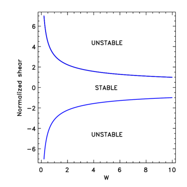
Figure 1: Map for the dynamo instability produced by the $\bar{\mbox{\boldmath$W$}}\times\bar{\mbox{\boldmath$J$}}$-effect. Field excitation can be found for sufficiently large positive values of the $W$-parameter (30).

3.1 Dynamos without stratification

Let the preferred direction $g$ be absent in a uniform original turbulence. Alpha-effect and pumping of magnetic field both vanish in this case. Nevertheless, a hydromagnetic dynamo by the $\bar{\mbox{\boldmath$W$}}\times\bar{\mbox{\boldmath$J$}}$-effect might be expected. Figure 1 shows the corresponding stability map. Dynamo excitation indeed exists for

$$W=\hat{\eta}_{y}\left(1+\pi^{2}\hat{\eta}_{x}\right)>0.$$ (30)

Note that after (10)₃ $\eta_{y}=\eta_{3}$ vanishes in the $\tau$-approximation or is otherwise negative-definite. Plane-shear flow dynamos are thus not possible in $\tau$-approximation – and they are also not possible without inclusion of $\eta_{x}$. Only the product $\eta_{x}\eta_{y}$ together with the overall shear allows the existence of plane-shear flow dynamos. No dynamo linear in the $\mbox{\boldmath$W$}\times\mbox{\boldmath$J$}$ term can exist in plane geometry.

For small Pm, however, $\eta_{x}$ is positive after Eq. (11)₂. Therefore also for the plane-shear flow (14) of liquid sodium or gallium ($\mathrm{Pm}\lower 1.72218pt\hbox{$\;\buildrel<\over{\scriptstyle\sim}\;$}10^{-5}$) a $\bar{\mbox{\boldmath$W$}}\times\bar{\mbox{\boldmath$J$}}$-slab-dynamo mechanism proves to be impossible. It would thus be challenging to probe the sign of the $\eta_{x}$ in the laboratory in accordance with the Eq. (17).

Another situation holds for the case of magnetic Prandtl number of order unity which is used in most of the numerical MHD simulations. As outlined above, the $\eta_{4}$ can then be negative if the frequency spectrum of the turbulence is steep enough (if it is too steep then $\eta_{3}$ vanishes!). A limiting magnetic Prandtl number between the two cases must exist and can be fixed by numerical integrations.

Figure 2: Stability map for a global dynamo solution of Eqs. (29) for $\hat{\Gamma}=-0.5$. Magnetic fields are excited in the parameters region above the lines. Solid: $\hat{\alpha}_{x}=\hat{\alpha}_{y}$, dashed: $\hat{\alpha}_{x}=0.1\hat{\alpha}_{y}$.

3.2 Dynamos with stratification

The $\alpha$-effect dynamos may be considered now ignoring the anisotropic dissipation in the Eqs. (29). For given shear, self-excitation of magnetic fields can be observed for sufficiently large $\hat{\alpha}_{y}$ and/or large enough shear. All the solutions are oscillatory. The oscillation time is of the order of the diffusion time for the case of isotropic $\alpha$-effect. In both considered cases a typical condition for dynamo excitation is

$$\hat{\alpha}_{y}\hat{S}>10.$$ (31)

(Fig. 2). A reformulation of this relation with $S\simeq\bar{u}/L$ yields

$${\rm Rm}>10\frac{L^{2}}{\alpha_{y}H},$$ (32)

where Rm=$L\bar{u}/\eta_{0}$ is the magnetic Reynolds number of the mean flow defined with the eddy diffusivity (8). The estimates $\eta_{0}\simeq u^{\prime}\ell_{\rm corr}/3$ and $\alpha_{y}\simeq\ell_{\rm corr}^{2}/H$ then reduce the inequality (32) to the condition

$$u^{\prime}<\frac{\bar{u}\ell_{\rm corr}}{3L}.$$ (33)

The fluctuating velocity should be sufficiently small to produce a dynamo. It cannot be too small, however, as the eddy diffusivity must remain larger than the microscopic one, $\eta_{0}>\eta$. This finally yields the condition

$$\frac{\eta}{\ell_{\rm corr}}<u^{\prime}<\frac{\bar{u}\ell_{\rm corr}}{3L},$$ (34)

which must be fulfilled for dynamo self-excitation. The microscopic magnetic diffusivity $\eta$ of liquid sodium or gallium is about $0.1$ m²/s. If the channel width, $L$, is as large as 1 m, then for the most optimistic case ($\ell_{\rm corr}\sim L$) the range (34) can be realized with shear velocities exceeding 1 m/s which is of the same order as in other dynamo experiments with a much more complicated geometry.

4 Summary

It is suggested that the basic effects of the theory of the turbulent dynamo which are usually concerned as special properties of rotating fluids can also be found for the plane shear flow. The same is probably true for any flow with global vorticity. The elementary structure of the shear flow largely simplifies the consideration. In the Appendix we have shown with the same concept as above that the generation of large-scale vorticity by a uniformly sheared turbulence is not possible and the generation of magnetic fields by such a flow can only be hoped for large magnetic Prandtl numbers.

The dynamo instability can be realized, however, when the turbulence is not uniform. Then the stratified turbulence produces the $\alpha$-effect which can excite an oscillatory mean magnetic field in the shear flow. This opens a possibility for the realization of a turbulent dynamo in the laboratory with a quite simple flow geometry – if a nonuniform turbulence can be created in the channel flow. Estimates of the excitation condition for such a dynamo, however, shows it to be at the limit of current experimental possibilities.

Appendix A Hydrodynamic stability of the shear flow

It is important for the above consideration that the linear shear flow (14) is hydrodynamically stable under the presence of nonlinear shear terms in the correlation tensor $Q_{ij}$. This question has been addressed by Elperin, Kleeorin and Rogashevskii (2003). With a dispersion relation formulated on the basis of (38, below) an instability has been constructed for plane wave disturbances with spatial inhomogeneity in the vertical $z$-direction. In contrast to this, we shall show that within the first-order smoothing approximation the shear flow is stable.

The one-point correlation tensor

$$Q_{ij}=\overline{u^{\prime}_{i}(\mbox{\boldmath$x$},t)u^{\prime}_{j}(\mbox{\boldmath$x$},t)}$$ (35)

in its linear form reads

$$Q_{ij}=P\delta_{ij}-\nu_{0}\left(\bar{u}_{i,j}+\bar{u}_{j,i}\right).$$ (36)

Here $\nu_{0}$ is the isotropic eddy viscosity; the turbulent pressure, $P$, includes all coefficients of the Kronecker tensor $\delta_{ij}$.

The experiment by Champagne et al. (1970) with sheared turbulence indicates that the linear relation (36) cannot be the whole truth. In the experiment the rms downstream velocities are systematically larger than the rms velocities in the cross-stream direction. The turbulence intensities for these two directions should, however, be equal after Eq. (36) which can be read as

$$\overline{u^{\prime 2}_{y}}=P,\quad\overline{u^{\prime 2}_{x}}=P,\quad\overline{u^{\prime}_{x}u^{\prime}_{y}}=-\nu_{0}S.$$ (37)

The same remains true if higher-order derivatives such as $\bar{u}_{i,jll}+\bar{u}_{j,ill}$ are included.

However, if the mean shear is indeed the only reason for anisotropy, one has also to involve nonlinear terms, i.e.

$$Q_{ij} = P\delta_{ij}-\nu_{0}\left(\bar{u}_{i,j}+\bar{u}_{j,i}\right)+\nu_{1}\bar{u}_{i,k}\bar{u}_{j,k}+$$ (38)

$$\ \ \ \ \ \ \ +\nu_{2}\bar{u}_{k,i}\bar{u}_{k,j}+\nu_{3}\left(\bar{u}_{i,k}\bar{u}_{k,j}+\bar{u}_{j,k}\bar{u}_{k,i}\right).$$

By this expression the horizontal intensities can differ if the coefficients $\nu_{1}$ and $\nu_{2}$ of the nonlinear terms do not coincide,

$$\overline{u^{\prime 2}_{y}}-\overline{u^{\prime 2}_{x}}=(\nu_{1}-\nu_{2})S^{2}.$$ (39)

It should be $\nu_{1}>\nu_{2}$ for agreement with the aforementioned shear-flow experiment.

The first-order term of Eq. (36) is the eddy viscosity

$$\nu_{0}=\frac{4}{15}\int\limits_{0}^{\infty}\!\!\int\limits_{0}^{\infty}\frac{\nu^{3}k^{6}E(k,\omega)}{(\omega^{2}+\nu^{2}k^{4})^{2}}{\rm d}k\ {\rm d}\omega,$$ (40)

(Krause & Rüdiger 1974). The second-order correction to the correlation tensor reproduce the nonlinear terms of (38). The coefficients $\nu_{1}$, $\nu_{2}$ and $\nu_{3}$ result as

$$\nu_{i}=\int\limits_{0}^{\infty}\!\!\int\limits_{0}^{\infty}K_{i}(k,\omega)E(k,\omega){\rm d}k\ {\rm d}\omega,\ \ \ n=1\dots 3\ ,$$ (41)

with the kernels

$$K_{1}=\frac{25\nu^{6}k^{12}+63\nu^{4}k^{8}\omega^{2}-149\nu^{2}k^{4}\omega^{4}+5\omega^{6}}{105\left(\omega^{2}+\nu^{2}k^{4}\right)^{4}},$$

$$K_{2}=\frac{4\left(8\nu^{6}k^{12}+7\nu^{4}k^{8}\omega^{2}-46\nu^{2}k^{4}\omega^{4}+3\omega^{6}\right)}{105\left(\omega^{2}+\nu^{2}k^{4}\right)^{4}},$$

$$K_{3}=\frac{25\nu^{6}k^{12}+49\nu^{4}k^{8}\omega^{2}-149\nu^{2}k^{4}\omega^{4}+19\omega^{6}}{105\left(\omega^{2}+\nu^{2}k^{4}\right)^{4}}.$$ (42)

All the kernels have negative (third) terms in their numerators. Nevertheless, all the coefficients (41) are ‘almost always’ positive. They are positive definite in the most popular simplifying cases, i.e.

– within the $\tau$-approximation:

$$\nu_{1}=\nu_{3}=\frac{5}{21}\ \tau_{\rm corr}\overline{u^{(0)2}},\ \ \nu_{2}=\frac{32}{105}\ \tau_{\rm corr}\overline{u^{(0)2}}$$ (43)

are always positive

– for white-noise spectra:

$$\nu_{1}=\nu_{2}=\frac{2\pi}{105\nu}\int\limits_{0}^{\infty}E(k)\frac{{\rm d}k}{k^{2}},\ \ \nu_{3}=\frac{\pi}{28\nu}\int\limits_{0}^{\infty}E(k)\frac{{\rm d}k}{k^{2}}$$ (44)

are always positive. The gap between (43) and (44) is filled by

$$E(k,\omega)=\frac{2}{\pi}\frac{w}{\omega^{2}+w^{2}}\hat{E}(k).$$ (45)

The coefficients (41) are positive-definite with (45).

For small disturbances, $\tilde{\mbox{\boldmath$u$}}$, of the mean flow depending on $z$ the cross correlations defined by (38) read

$$Q_{xz} = -\nu_{0}D\tilde{u}_{x}+\nu_{2}SD\tilde{u}_{y},$$

$$Q_{yz} = -\nu_{0}D\tilde{u}_{y}+\nu_{3}SD\tilde{u}_{x}.$$ (46)

The linear equation system for the disturbances is

$$\frac{\partial\tilde{u}_{x}}{\partial t} - \nu_{0}D^{2}\tilde{u}_{x}+\nu_{2}SD^{2}\tilde{u}_{y}=0,$$

$$\frac{\partial\tilde{u}_{y}}{\partial t} + S\tilde{u}_{x}-\nu_{0}D^{2}\tilde{u}_{y}+\nu_{3}SD^{2}\tilde{u}_{x}=0.$$ (47)

It reduces to

$$\left(\nu_{2}\nu_{3}S^{2}-\nu_{0}^{2}\right)D^{2}\tilde{u}_{x}+\nu_{2}S^{2}\tilde{u}_{x}=0$$ (48)

in the stationary case. The 1D problem should be accomplished by boundary conditions imposed at (say) $z=0$ and $z=H$. But Eq. (48) possesses a solution only if

$$H=\pi\sqrt{\frac{\nu_{0}^{2}-\nu_{2}\nu_{3}S^{2}}{-\nu_{2}S^{2}}}$$ (49)

irrespectively of whether no-slip or stress-free boundary conditions are applied. The second term in the numerator of (49) must be small compared to the first one. Otherwise the nonlinear correlations (38) which neglect the third and higher order terms in the mean shear cannot be applied. Therefore, an instability only exists for $\nu_{2}<0$. The quantity $\nu_{2}$ proved to be positive for almost all spectra. The shear flow (14) thus proves to be stable in the hydrodynamic regime.