On the Robustness of the Acoustic Scale
in the Low-Redshift Clustering of Matter

Abstract

We discuss the effects of non-linear structure formation on the signature of acoustic oscillations in the late-time galaxy distribution. We argue that the dominant non-linear effect is the differential motion of pairs of tracers separated by 150 Mpc. These motions are driven by bulk flows and cluster formation and are much smaller than the acoustic scale itself. We present a model for the non-linear evolution based on the distribution of pairwise Lagrangian displacements that provides a quantitative model for the degradation of the acoustic signature, even for biased tracers in redshift space. The Lagrangian displacement distribution can be calibrated with a significantly smaller set of simulations than would be needed to construct a precise power spectrum. By connecting the acoustic signature in the Fourier basis with that in the configuration basis, we show that the acoustic signature is more robust than the usual Fourier-space intuition would suggest because the beat frequency between the peaks and troughs of the acoustic oscillations is a very small wavenumber that is well inside the linear regime. We argue that any possible shift of the acoustic scale is related to infall on 150 Mpc scale, which is $O(0.5\%)$ fractionally at first-order even at $z=0$. For the matter, there is a first-order cancellation such that the mean shift is $O(10^{-4})$. However, galaxy bias can circumvent this cancellation and produce a sub-percent systematic bias.

1 Introduction

The imprint in the late-time clustering of matter from the baryon acoustic oscillations in the early Universe (Peebles & Yu, 1970; Sunyaev & Zel’dovich, 1970; Doroshkevich, Zel’dovich, & Sunyaev, 1978) has emerged as an enticing way to measure the distance scale and expansion history of the Universe (Eisenstein, Hu, & Tegmark, 1998; Cooray, Hu, Huterer & Joffre, 2001; Eisenstein, 2003; Blake & Glazebrook, 2003; Hu & Haiman, 2003; Seo & Eisenstein, 2003; Linder, 2003; Matsubara, 2004; Amendola et al., 2005; Blake & Bridle, 2005; Glazebrook & Blake, 2005; Dolney, Jain, & Takada, 2006). The distance that acoustic waves can propagate in the first million years of the Universe becomes a characteristic scale, measurable not only in the CMB anisotropies (Miller et al., 1999; de Bernardis et al., 2000; Hanany et al., 2000; Halverson et al., 2002; Netterfield et al., 2002; Bennett et al., 2003) but also in the late-time clustering of galaxies (Cole et al., 2005; Eisenstein et al., 2005). This scale can be computed with simple linear perturbation theory once one specifies the baryon-to-photon ratio and matter-radiation ratio, both of which can be measured from the details of the CMB acoustic peaks (Bennett, Turner, & White, 1997; Hu et al., 1997; Hu & Dodelson, 2002; White & Cohn, 2002). With this scale in hand, one can measure the angular diameter distance and Hubble parameter as functions of redshift using large galaxy redshift surveys. This standard ruler offers a robust route to the study of dark energy.

However, the clustering of galaxies does not exactly recover the linear-theory clustering pattern. Non-linear gravitational collapse, galaxy clustering bias, and redshift distortions all modify galaxy clustering relative to that of the linear-regime matter correlations. In particular, simulations have shown that non-linear structure formation and, to a lesser extent, redshift distortions erase the higher harmonics of the acoustic oscillations (Meiksin et al., 1999; Seo & Eisenstein, 2005; Springel et al., 2005; White, 2005). This degrades the measurement of the acoustic scale. More worrisome is the possibility that these effects might actually bias the measurement.

In this paper, we present a physical explanation of these non-linear distortions. We use a hybrid of analytic and numerical methods to produce a quantitative model for the degradation. We also investigate whether the non-linearities can measurably shift the acoustic scale. The results offer the opportunity to calibrate the effects of non-linearities with simulations far smaller than what would be required to see the effects directly in the acoustic signature.

We organize the paper as following. In § 2, we present a pedagogical review of the acoustic phenomenon, explaining the effects in both the configuration and Fourier bases. In § 3, we discuss how non-linearities enter the process and why the large preferred scale of the acoustic oscillations provides an important simplification of the dynamics. In § 4, we present a quantitative framework for understanding the non-linear effects based on Lagrangian displacements. We construct Zel’dovich approximation estimates of the displacements in § 5 and then measure the required distributions numerically and compare them to the non-linear two-point functions in § 6. The model is extended to biased tracers in § 7. In § 8, we study how non-linearities could create systematic shifts in the acoustic scale. We conclude in § 9.

Throughout the paper, we will refer to redshift space as the position of galaxies or matter inferred from redshifts, with no correction for peculiar velocities. The true position of the galaxies or matter will be called real space. Sometimes, the term real space is used in cosmology as the complement to the Fourier basis; we will instead refer to these as Fourier and configuration space (or basis) to avoid confusion. We use comoving distance units in all cases.

2 Acoustic oscillations in configuration and Fourier space

This section is pedagogical in nature. The physics of the acoustic oscillations have been well studied in Fourier space, but we have found that the story in configuration space is rarely discussed even though it exhibits some of the most important features for our purposes. Moreover, this pedagogy can warm up the reader to the configuration-space view of the non-linearities that we pursue in the rest of the paper.

The epoch of recombination marks the time when the Universe has cooled enough that protons and electrons combine to form hydrogen (Peebles, 1968; Zel’dovich, Kurt, & Sunyaev, 1969; Seager, Sasselov, & Scott, 1999). Prior to this time, the mean free path of the photons against scattering off of the free electrons is much less than the Hubble distance. This means that gravitational forces attempting to compress the plasma must also increase the photon density. This produces an increase in temperature and hence in radiation pressure. Any perturbation in the baryon-photon plasma thus behaves as an acoustic wave.

2.1 Fourier space

Before looking at this picture in configuration space, let us remind ourselves of the physics in Fourier space. Consider a (standing) plane wave perturbation of comoving wavenumber $k$ in Newtonian gauge (e.g. Kodama & Sasaki, 1984). At early times, the density is high and the scattering is rapid compared with the travel time across a wavelength. We may therefore expand the momentum conservation (Euler) equation in powers of the Compton mean free path over the wavelength $k/\dot{\tau}$, where $\dot{\tau}$ is the differential Compton optical depth and overdots denote derivatives with respect to conformal time $\eta=\int dt/a$. To lowest order and setting $c=1$, we obtain the tight coupling approximation for the evolution of a single Fourier mode of the baryon density perturbation [Peebles & Yu (1970); Doroshkevich, Zel’dovich, & Sunyaev (1978) or for a more recent derivation in the relevant gauge and notation Hu & White (1996)]

$${d\over d\eta}\left[(1+R)\dot{\delta}_{b}\right]+{k^{2}\over 3}\delta_{b}=-k^{2}(1+R)\Psi-{d\over d\eta}\left[3(1+R)\dot{\Phi}\right].$$ (1)

Here $R\equiv 3\rho_{b}/4\rho_{\gamma}$ is the baryon-to-photon momentum density ratio and the gravitational sources are $\Phi$, the perturbation to the spatial curvature, and $\Psi$, the Newtonian potential. At late times, the gravitational perturbations are dominated by the CDM and baryons (if $\Omega_{b}/\Omega_{m}$ is large), while at early times they are dominated by the relativistic species. We recognize this equation as that of a driven oscillator with natural frequency $c_{s}k$, where the speed of sound $c_{s}$ is $c/\sqrt{3(1+R)}$. During the tight coupling phase, the amplitude of the baryon perturbations cannot grow and instead undergoes harmonic motion with an amplitude that decays as $(1+R)^{-1/4}$ and a velocity that decays as $(1+R)^{-3/4}$ (Hu & Sugiyama, 1995; Hu & White, 1996). For currently accepted values of $\Omega_{b}$ (Spergel et al., 2006; Steigman, 2006), $R<0.3$ at $z>1000$ so the decay of the period is small.

If we define the optical depth $\tau_{b}(\eta)\equiv\int_{\eta}^{\rm today}\ d\eta\;\dot{\tau}/(1+R)$, we find that the baryons decouple from the photons when $\tau_{b}\sim 1$, a time we shall refer to as “decoupling”. The oscillations in the baryons are frozen in at this epoch, which occurs after recombination for currently accepted values of $\Omega_{b}$. Expanding to higher order in $k/\dot{\tau}$, one finds the oscillations are exponentially damped to due photon-baryon diffusion (Silk, 1968) with a characteristic scale which is approximately the geometric mean of the horizon and the mean free path at decoupling (of order $10$ Mpc for a concordance cosmology). Including the finite duration of recombination slightly alters the damping from this exponential form (Hu & White, 1997), but this detail will not be of relevance to us here. Note that since decoupling occurs slightly after recombination, both the sound horizon and the damping scale are slightly larger than the corresponding scales in the CMB.

Once the photons release their hold on the baryons, the latter can be treated as pressureless allowing the perturbations to grow by gravitational instability (e.g. proportionally to the scale factor in a matter-dominated Universe). The density and velocity perturbations from the tight-coupling era, including the CDM perturbations, must be matched onto the growing and decaying modes for the pressureless components. The final spectrum is the component which projects onto the growing mode. As is well known (Sunyaev & Zel’dovich, 1970; Press & Vishniac, 1980) — see Padmanabhan (1993), §8.2 for a textbook treatment — at high $k$ the growing mode is sourced primarily by the velocities, while at low $k$ it is a mixture of density and velocity terms. For this reason, at high $k$ the oscillations in the mass power spectrum are out of phase with the peaks in the CMB anisotropy spectrum, which arise predominantly from photon densities. In this limit, extrema occur at $ks_{*}=(2j+1)\pi/2$ where $j=0,1,2,\ldots$ and $s_{*}$ is the sound horizon at decoupling: $s_{*}=\int c_{s}\,d\eta$. In detail, this differs from the sound horizon at recombination (which controls the position of the CMB peaks) but the two horizons are comparable. The amplitude of the oscillations depends on both the driving force ($\Phi$ and $\Psi$) and on $R$. Since the potentials decay in the radiation-dominated epoch, larger oscillations come from higher $\Omega_{b}h^{2}$ and lower $\Omega_{m}h^{2}$ (Eisenstein & Hu, 1998; Meiksin et al., 1999).

2.2 Configuration space

 

 

 

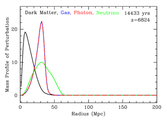
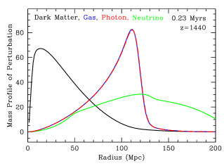
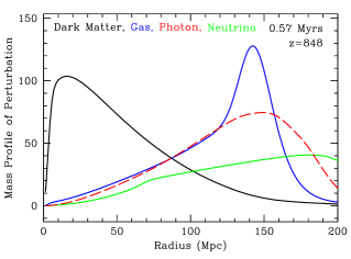
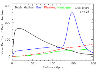
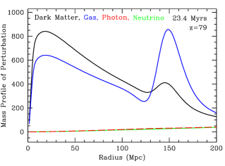
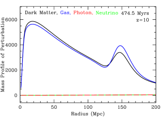
Figure 1: Snapshots of evolution of the radial mass profile versus comoving radius of an initially point-like overdensity located at the origin. All perturbations are fractional for that species; moreover, the relativistic species have had their energy density perturbation divided by 4/3 to put them on the same scale. The black, blue, red, and green lines are the dark matter, baryons, photons, and neutrinos, respectively. The redshift and time after the Big Bang are given in each panel. The units of the mass profile are arbitrary but are correctly scaled between the panels for the synchronous gauge. a) Near the initial time, the photons and baryons travel outwards as a pulse. b) Approaching recombination, one can see the wake in the cold dark matter raised by the outward going pulse of baryons and relativistic species. c) At recombination, the photons leak away from the baryonic perturbation. d) With recombination complete, we are left with a CDM perturbation towards the center and a baryonic perturbation in a shell. e) Gravitational instability now takes over, and new baryons and dark matter are attracted to the overdensities. f) At late times, the baryonic fraction of the perturbation is near the cosmic value, because all of the new material was at the cosmic mean. These figures were made by suitable transforms of the transfer functions created by CMBfast (Seljak & Zaldarriaga, 1996; Zaldarriaga & Seljak, 2000).

With this in mind, it is instructive to switch to configuration space and consider what happens to a point-like initial overdensity. In an adiabatic model, the overdensity is present in all species (Peebles & Yu, 1970). In particular, because the region is overdense in photons, it is overpressured relative to its surroundings. This overpressure must equilibrate by driving a spherical sound wave out into the baryon-photon plasma. The cold dark matter perturbation is left at small radius. The sound wave travels out at the speed of sound. At the time of decoupling, the wave stalls as the pressure-supplying photons escape and the sound speed plummets. One ends up with a CDM overdensity at the center and a baryon overdensity in a spherical shell 150 comoving Mpc in radius for the concordance cosmology. At $z\ll 10^{3}$, both of these overdensities attract gas and CDM to them, seeding the usual gravitational instability (Peebles & Yu, 1970). The fraction of gas to CDM approaches the cosmic average as the perturbation grows by a factor approaching $10^{3}$, so that one ends up with an overdensity of all matter at the center and a spherical echo at 150 Mpc radius. Galaxies are more likely to form in these overdensities. The radius of the sphere marks a preferred separation of galaxies, which we quantify as a peak in the correlation function on this scale. This evolution is shown graphically in Figure 1.

The Universe is of course a superposition of these point-like perturbations, but as the perturbation theory is exquisitely linear at high redshift, we can simply add the solutions. The width of the acoustic peak is set by three factors: Silk damping due to photons leaking out of the sound wave (Silk, 1968), adiabatic broadening of the wave as the sound speed changes due to the increasing inertia of the baryons relative to the photons, and the correlations of the initial perturbations. In practice, the acoustic peak is about 30 Mpc full width at half maximum for the concordance cosmology.

There are some other interesting aspects of the physics of this epoch that are worth mentioning in the configuration-space picture. First is that the outgoing wave does not actually stop at $z\sim 10^{3}$ but instead slows around $z\sim 500$. This is partially due to the fact that decoupling is not coincident with recombination but is also because the coupling to the growing mode is actually dominated by the velocity field, rather than the density field, at $z\sim 10^{3}$ (Sunyaev & Zel’dovich, 1970; Press & Vishniac, 1980). In other words, the compressing velocity field in front of the wave actually keys the instability at later time.

Two other aspects of Figure 1 that may be surprising at first glance are that the outgoing pulse of neutrino overdensity doesn’t actually remain as a delta function, as one might expect for a population traveling radially outward at the speed of light, and that the CDM perturbation doesn’t remain at the origin, as one would expect for a cold species. Both of these effects are due to a hidden assumption in the initial conditions: although the density field is homogeneous everywhere but the origin, the velocity field cannot be for a growing mode. To keep the bulk of the universe homogeneous while growing a perturbation at the origin matter must be accelerating towards the center; this acceleration is supplied by the gravitational force from the central overdensity. However, in the radiation-dominated epoch the outward going pulse of neutrinos and photons is carrying away most of the energy density of the central perturbation. This outward going pulse decreases the acceleration, causing the inward flow of the homogeneous bulk to deviate from the divergenceless flow and generating the behavior of the CDM and neutrinos mentioned above. Essentially the outgoing shells of neutrinos and photons raise a wake in the homogeneous distribution of CDM away from the origin of the perturbation.

The smoothing of the CDM overdensity from a delta function at the origin is the famous small-scale damping of the CDM power spectrum in the radiation-dominated epoch (Lifshitz, 1946; Peebles & Yu, 1970; Sunyaev & Zel’dovich, 1970; Groth & Peebles, 1975; Doroshkevich, Zel’dovich, & Sunyaev, 1978; Wilson & Silk, 1981; Peebles, 1981; Blumenthal et al., 1984; Bond & Efstathiou, 1984). The overdensity raised decreases as a function of radius because the radiation is decreasing in energy density relative to the inertia of the CDM; in the matter-dominated regime, the outward-going radiation has no further effect. A Universe with more radiation causes a larger effect that extends to larger radii; this corresponds to the shift in the CDM power spectrum with the matter-to-radiation ratio.

Returning to the major conceptual point, that of the shell of overdensity left at the sound horizon, we see immediately that the sound horizon provides a standard ruler. The radius of the shell depends simply on the sound speed and the amount of propagation time (Peebles & Yu, 1970; Sunyaev & Zel’dovich, 1970; Doroshkevich, Zel’dovich, & Sunyaev, 1978). The sound speed is set by the balance of radiation pressure and inertia from the baryons; this is controlled simply by the baryon-to-photon ratio, which is $\Omega_{b}h^{2}$. The propagation time depends on the expansion rate in the matter-dominated and radiation-dominated regimes; this depends on the redshift of matter-radiation equality, which depends only on $\Omega_{m}h^{2}$ for the standard assumption of the radiation density (i.e., the standard cosmic neutrino and photon backgrounds and nothing else).

2.3 Connecting Fourier & Configuration space

Next, it is useful to connect this picture to the Fourier space view of the evolution of plane waves. Here we consider not standing waves, where the accumulated phase change until decoupling determines the positions of the peaks in the power spectrum, but traveling waves. We imagine each overdense crest of the initial perturbation launches a planar sound wave that travels out for 150 Mpc (Bashinsky & Bertschinger, 2001, 2002). If this places the baryon perturbation on top of another crest in the initial wave (now marked by the CDM), then one will get constructive interference in the density field and a peak in the power spectrum. If the sound wave lands in the trough of the initial wave, then one gets a destructive interference. Hence, one gets a harmonic pattern of oscillations, with a damping set by the width of the post-recombination baryon and CDM perturbations from a thin initial plane (i.e. the 1-d Green’s function).

In our opinion, for understanding the late-time matter spectrum, in particular the standard ruler aspect, the traveling wave view has considerable pedagogical advantages. The fact that the baryon signature in the correlation function has a single peak is a provocative indication that the physics is easily viewed as the causal propagation of a signal. Mathematically, the connection is that the correlation function and power spectrum are Fourier transform pairs. The transform of a single peak is a harmonic sequence, and the profile of the peak gives the damping envelope of the oscillations. We shall draw upon this picture as we consider non-linear evolution in the following sections.

3 The non-linear degradation of the acoustic signature

At low redshift, non-linear structure formation, redshift distortions, and galaxy clustering bias all act to degrade the acoustic signature in the galaxy power spectrum (Meiksin et al., 1999; Seo & Eisenstein, 2005; Springel et al., 2005; White, 2005). These effects reduce the amount of distance-scale information that can be extracted from a survey of a given volume (Seo & Eisenstein, 2003; Blake et al., 2006). In principle, they might also shift the scale, resulting in biased information from uncorrected estimators. One should of course distinguish such shifts from a simple increase in noise; a noisy statistical estimator is not the same as a biased one.

How do the breakdowns of the ideal linear case enter? We begin in Fourier space. Here the acoustic signature is a damping harmonic series of peaks and troughs. As non-linearities progress, mode-mode coupling begins to alter the power spectrum. Power increases sharply at large wavenumber, but the mode-mode coupling also damps out the initial power spectrum on intermediate scales, decreasing the acoustic oscillations (Goroff et al., 1986; Jain & Bertschinger, 1994; Meiksin et al., 1999; Jeong & Komatsu, 2006). Both of these effects reduce the contrast of the oscillations, making them harder to measure.

At $z<1$, N-body simulations and galaxy catalogs derived therefrom show an excess of power at the location of the higher acoustic harmonics ($k\approx 0.2h{\rm\,Mpc}^{-1}$). Clearly the non-linear power spectrum deviates from the linear one at wavenumbers containing acoustic information. Does this mean that one cannot recover “linear” information from these scales? As we’ll see next, the answer is not this pessimistic.

In configuration space, the acoustic signature is a single peak in the correlation function at $150{\rm\,Mpc}$ separation. The width of the peak is related to the decreasing envelope of the oscillations in the power spectrum. The action of the non-linear effects is easy to see: velocity flows and non-linear collapse move matter in the Universe around by of order $10{\rm\,Mpc}$ relative to its initial comoving position. This tends to move pairs out of the $150{\rm\,Mpc}$ peak, broadening it. This broadening corresponds to the decay of the high harmonics in $P(k)$. One also sees that because redshift distortions further increase the distance between a galaxy’s measured position and its initial position, the acoustic oscillations are further reduced in redshift space.

The key insight from the configuration-space picture is that the processes that are erasing the acoustic signature are not at the fundamental scale of $150{\rm\,Mpc}$ but are at the cluster-formation scale, a factor of 10 smaller. This is very different from the apparent behavior in Fourier space that suggests the non-linearities are encroaching on the acoustic scale. The solution to the paradox is to note that the acoustic information in Fourier space is actually carried by the comparison of adjacent peaks and troughs. The beat frequency between these nearby wavenumbers is much smaller, about $\Delta k=0.03h{\rm\,Mpc}^{-1}$, and is well below the non-linear wavenumber. In other language, the power that is being built by mode-mode coupling must be smooth on the scale of $\Delta k$ because the non-linearities are developing on much smaller scales. The existence of this small beat frequency changes the behavior of non-linearities relative to our usual intuition, which are based on broad-band effects.

It is also interesting to note that the power that is being introduced by halo formation on small scales is particularly smooth at the wavenumbers of interest (Schulz & White, 2006). In the correlation function, this non-linearity adds very little to $\xi$ at the acoustic scale; it is purely an excess correlation on halo scales. This reinforces the idea that such power can be removed by marginalizing over smooth broadband spectra without biasing the recovery of the acoustic scale. The important effect of the small-scale non-linearity is the increase in noise. This is clear in the power spectrum, where the noise even in the Gaussian limit is increased by the extra near-white noise at small wavenumbers. It is less obvious in the correlation function, as $\xi(r)$ itself has not changed on the acoustic scale. However, the noise will be present in the covariance matrix of the correlation function, as the near-white noise acts as extra shot noise that increases the variance in the correlation function.

As for the acoustic scale itself, in configuration space, it is easy to see that it will not be shifted much at all. The scale of $150{\rm\,Mpc}$ is far larger than any known non-linear effect in cosmology. To shift the peak, we need to imagine effects that would systematically move pairs at $150{\rm\,Mpc}$ to smaller or larger separations. We will return to this point in detail in §8 and argue that non-linear gravitational physics can only introduce shifts of order 0.5% even at first order and that linearly biased tracers imply a cancellation of the first-order term.

Hence, the picture of the non-linear evolution of the acoustic signature is easy to see in configuration space: the characteristic separation of $150{\rm\,Mpc}$ is not shifted but rather is blurred by the action of cluster formation and bulk flows that move matter around by $\sim\!10{\rm\,Mpc}$. This smears out the peak in the correlation function, further damping out the higher harmonics in the power spectrum. The acoustic scale becomes harder to measure in a survey because the wider correlation peak is harder to centroid or because the higher harmonics are at lower contrast in the power spectrum. The existence of collapsed halos adds extra near-white noise in the power spectrum and creates increased variance in measurements of the correlation function.

Again, there is nothing in the configuration-space version of the story that can’t be stated in the Fourier-space version, but one must remember that the small beat frequency between the peaks and troughs of the acoustic oscillations means that one’s usual intuition about broadband Fourier effects doesn’t fully apply. In particular, the fact that the power spectrum does show non-linear alterations at $k=0.1$–$0.2h{\rm\,Mpc}^{-1}$ does not mean that the acoustic effects are hopelessly muddied by non-linearities.

4 Modeling the degradation as a Lagrangian displacement

We have argued that the erasure of the acoustic signature can be understood as being due to the motions of matter and galaxies relative to the initial preferred separation. It is therefore interesting to think about the displacement of matter or tracers from their position in the near-homogeneous initial state. This is the Lagrangian displacement, well known from the Zel’dovich approximation (Zel’dovich, 1970).

We write the Lagrangian displacement as a vector $\vec{u}(\vec{r})$, where $\vec{r}$ is the comoving coordinate system for the homogeneous cosmology. One can then write the correlation function at a particular (large) separation as

$$\xi(\vec{s})=\int d\vec{r}_{12}\,d\vec{u}_{12}\,d\delta_{1}\,d\delta_{2}\,p(\delta_{1},\delta_{2})\,\delta_{1}\delta_{2}\,p(\vec{u}_{12}|\vec{r}_{12},\delta_{1},\delta_{2})\,\delta^{(3)}(\vec{r}_{12}+\vec{u}_{12}-\vec{s})$$ (2)

where the subscripts 1 and 2 indicate the density values at two different points, $\vec{r}_{12}=\vec{r}_{1}-\vec{r}_{2}$, and likewise for $\vec{u}_{12}$. The probability distribution $p(\delta_{1},\delta_{2})$ is the distribution of the initial density field; on large scales, there is a small correlation $\xi(\vec{r}_{12})$ between the densities. The probability distribution $p(\vec{u}_{12}|\vec{r}_{12},\delta_{1},\delta_{2})$ is the distribution for the Lagrangian displacements. If one were considering local clustering bias, then one could replace the product $\delta_{1}\delta_{2}$ by a stochastic bias $\delta_{g,1}\delta_{g,2}p(\delta_{g,1}|\delta_{1})p(\delta_{g,2}|\delta_{2})$.

In general, this integral is similar to the general redshift distortion problem (Hamilton, 1998; Scoccimarro, 2004; Matsubara et al., 2004) and does not have an easy solution. In practice, given how large the desired scale is compared to the scale of cluster formation and likely galaxy physics, we consider a peak-background split. For this, we write the density field as a sum of a large-amplitude small-scale density field $\delta^{S}$ and a small-amplitude large-scale density field $\delta^{L}$. These fields are to be thought of as statically independent. The small-scale fields at the two points will be statistically independent. We do similarly for the Lagrangian displacement field. This yields

$$\xi(\vec{s}) = \int d\vec{r}_{12}\,d\vec{u}_{1}^{S}\,d\vec{u}_{2}^{S}\,d\vec{u}_{12}^{L}\,d\delta_{1}^{S}\,d\delta_{2}^{S}\,d\delta_{1}^{L}\,d\delta_{2}^{L}\,\,p(\delta_{1}^{L},\delta_{2}^{L})\,p(\delta_{1}^{S})p(\delta_{2}^{S})\,(\delta_{1}^{S}+\delta_{1}^{L})(\delta_{2}^{S}+\delta_{2}^{L})$$ (3)

$$p(\vec{u}_{1}^{S}|\delta_{1}^{S})\,p(\vec{u}_{2}^{S}|\delta_{2}^{S})\,p(\vec{u}_{12}^{L}|\vec{r}_{12},\delta_{1}^{L},\delta_{2}^{L})\,\delta^{(3)}(\vec{r}_{12}+\vec{u}_{12}^{L}+\vec{u}_{1}^{S}-\vec{u}_{2}^{S}-\vec{s})$$

Only the $\delta_{1}^{L}\delta_{2}^{L}$ cross-term yields a non-zero result.

If we treat the large-scale Lagrangian displacement as a delta function at $\vec{u}_{12}^{L}=0$ for the moment, then this integral reduces simply to

$$\xi(\vec{s})=\int d\vec{r}_{12}\xi(\vec{r}_{12})\int d\delta_{1}^{S}\,d\vec{u}_{1}^{S}\,p(\delta_{1}^{S})\,p(\vec{u}_{1}^{S}|\delta_{1}^{S})\int d\delta_{2}^{S}\,d\vec{u}_{2}^{S}\,p(\delta_{2}^{S})\,p(\vec{u}_{2}^{S}|\delta_{2}^{S})\,\delta^{(3)}(\vec{r}_{12}+\vec{u}_{1}^{S}-\vec{u}_{2}^{S}-\vec{s}).$$ (4)

In other words, this is simply the correlation function convolved twice with the distribution $p(\vec{u}^{S})$ of small-scale Lagrangian displacements. This function can depend on the galaxy bias model. In the case of the redshift-space correlation function, one can simply treat $p(\vec{u}^{S})$ as the difference between the initial position (which is the same in real or redshift space) and the final position in redshift space; the function obviously becomes anisotropic in this case. When computing the small-scale displacement field $\vec{u}^{S}$, one should high-pass filter to remove bulk flows on scales at or larger than $|\vec{s}|$. This correction is important, because bulk flows are generated on quite large scales in CDM cosmologies.

Of course, the double convolution of the correlation function is a trivial multiplication in the power spectrum. Either way, one sees that the small-scale power has been strongly suppressed. One should remember that this procedure only represents the memory of the initial correlation pattern; it does not introduce the small-scale non-linear clustering that builds up the small-scale correlation function or power spectrum.

We do not have a full solution to the case with an arbitrary large-scale Lagrangian displacement field. However, we find a significant simplification in equation (2) or (3) if we assume that the distribution of $\vec{u}_{12}$ or $\vec{u}_{12}^{L}$ is independent of $\delta_{1}$ and $\delta_{2}$. This is not true in detail: overdense regions will tend to move toward one another, underdense regions away. The mean $\vec{u}_{12}$ depends on $\delta_{1}^{L}+\delta_{2}^{L}$ at linear order, but as shown in § 8, the amount of this shift is much less than the $30{\rm\,Mpc}$ width of the acoustic peak. It is also much less than the standard deviation of the $\vec{u}_{12}$ distribution computed in § 5 or measured in § 6. Hence, because the shifts are small and because the density dependence produces opposing shifts between the overdense and underdense regions, it is a good approximation to ignore the dependence when computing the broadening of the acoustic peak. This would of course not be a good approximation for determining whether there is a mean shift in the scale; we will return to this topic in §8.

As both the large and small-scale terms have boiled down to the distribution of displacements unconditioned by the density field, we suggest that one can handle both of the effects simultaneously and also do the proper filtering of the large-scale bulk flows by computing the distribution of $\vec{u}_{12}$ for pairs of particles separated by a given $\vec{r}_{12}$, without regard for the dependence on $\delta_{1}$ and $\delta_{2}$. Note that this avoids computing a peak-background split. The resulting distribution $p(\vec{u}_{12}|\vec{r}_{12})$ is our model for the kernel that the correlation function will be convolved with, following equation (2). We will measure this kernel numerically in §6 and show that it reproduces the non-linear degradation of the acoustic signatures in simulated power spectra.

If we consider a local clustering bias (Coles, 1993; Scherrer & Weinberg, 1998; Dekel & Lahav, 1999), then we can write

$$\xi(\vec{s})=\int d\vec{r}_{12}\,d\vec{u}_{12}\,d\delta_{1}\,d\delta_{2}\,p(\delta_{1},\delta_{2})\,d\delta_{g,1}\,d\delta_{g,2}\,p(\delta_{g,1}|\delta_{1})\,p(\delta_{g,2}|\delta_{2})\delta_{g,1}\delta_{g,2}\,p(\vec{u}_{12}|\vec{r}_{12},\delta_{1},\delta_{2})\,\delta^{(3)}(\vec{r}_{12}+\vec{u}_{12}-\vec{s})$$ (5)

where $\vec{u}$ refer the displacements of the galaxies. In the peak-background split, the $\delta_{g,1}$ factor becomes $\delta_{g,1}^{S}+b\delta_{1}^{L}$, where $b$ is the large-scale bias. In equation (4), the terms of the form

$$\int d\delta_{1}^{S}\,d\vec{u}_{1}^{S}p(\delta_{1}^{S})\,p(\vec{u}_{1}^{S}|\delta_{1}^{S})$$ (6)

become

$$b\int d\delta_{1}^{S}\,d\delta_{g,1}\,d\vec{u}_{1}^{S}\,p(\delta_{1}^{S})\,p(\delta_{g,1}^{S}|\delta_{1}^{S})\,p(\vec{u}_{1}^{S}|\delta_{1}^{S}).$$ (7)

In a simulation, this reduces to the distribution of $\vec{u}_{1}$ for galaxy “particles”. Again, we suggest simply computing $\vec{u}_{1}-\vec{u}_{2}$ for pairs of galaxies separated by $\vec{r}_{12}$. Of course, the initial position of a galaxy is ill-defined in a simulation, but as we are interested in displacements similar in size to the width of the acoustic peak, we expect that any reasonable measure of the initial position of the center of mass of the galaxy will agree to better than 1 Mpc, which is negligible in the scatter of the displacements. It is important to note that the distribution of the displacements of the galaxies may be different from that of the mass displacement, particularly in redshift space.

The picture of a peak and a spherical echo might lead one to hope that one could pick tracers that would preferentially accentuate the peak or sphere, therefore boosting the height of the peak in the correlation function. We show explicitly in Appendix A that this is not possible for local bias, at least within the Gaussian random field assumption; the large-scale correlation function of galaxies always tracks that of the matter, as known from theorems about local bias (Coles, 1993; Scherrer & Weinberg, 1998).

5 Analytic Estimates

In the Zel’dovich approximation our interest in the Lagrangian displacements translates into study of correlations in the initial velocity field at two points. The displacement is

$$\vec{u}_{12}=\int{d\vec{k}\over(2\pi)^{3}}\delta_{\vec{k}}{\vec{k}\over ik^{2}}\left[e^{i\vec{k}\cdot\vec{r}_{1}}-e^{i\vec{k}\cdot\vec{r}_{2}}\right].$$ (8)

This quantity has a mean of zero, but of course the variance is non-zero. The variance of the displacement along the direction between the two points is

$$\left\langle u_{12,\parallel}^{2}\right\rangle=\int{d\vec{k}\over(2\pi)^{3}}P(k)\left(\vec{k}\cdot\vec{r}_{12}\over k^{2}r_{12}\right)^{2}\left|e^{i\vec{k}\cdot\vec{r}_{12}}-1\right|^{2}=r_{12}^{2}\int{k^{2}\,dk\over 2\pi^{2}}P(k)f_{\parallel}(kr_{12})$$ (9)

where

$$f_{\parallel}(x)={2\over x^{2}}\left({1\over 3}-{\sin x\over x}-{2\cos x\over x^{2}}+{2\sin x\over x^{3}}\right).$$ (10)

Note that $f_{||}\rightarrow 1/5-x^{2}/84$ as $x\rightarrow 0$, so the result behaves similarly as $k\rightarrow 0$ as the integral to compute the density fluctuations, rather than the $k^{-2}$ behavior of the rms bulk flow integrand. This is because very large wavelength modes move both particles together. The variance of the displacement in a direction orthogonal to $\vec{r}_{12}$ is the same formula, but with

$$f_{\perp}(x)={2\over x^{2}}\left({1\over 3}-{\sin x\over x^{3}}+{\cos x\over x^{2}}\right),$$ (11)

which behaves as $1/15-x^{2}/420$ as $x\rightarrow 0$.

For a concordance CDM cosmology with $\sigma_{8}=0.85$ (i.e., $z\approx 0$), we find rms displacements of $9h^{-1}{\rm\,Mpc}$ along the separation direction and $8h^{-1}{\rm\,Mpc}$ transverse for separations of $100h^{-1}{\rm\,Mpc}$. These displacements are mostly generated on large scales, with 50% of the variance at $k<0.05h{\rm\,Mpc}^{-1}$ for radial displacements and $k<0.08h{\rm\,Mpc}^{-1}$ for transverse. Rather little of the variance is generated at $k<0.02h{\rm\,Mpc}^{-1}$; wavelengths much longer than $100h^{-1}{\rm\,Mpc}$ move both points similarly. The displacements scale linearly with $\sigma_{8}$ (of the matter) and hence are smaller at high redshift.

In redshift space, the Lagrangian displacement in the Zel’dovich approximation is simply increased by a factor of $f=d(\ln D)/d(\ln a)\approx\Omega_{m}^{0.56}$ along the line of sight, because the same velocity that gives the real-space displacement also alters the position in redshift space (Peebles, 1980; Kaiser, 1987).

6 Numerical Results for the Matter Distribution

Figure 2: The distribution of pairwise Lagrangian displacements for particles initially separated by $100h^{-1}{\rm\,Mpc}$. The left panel is in real space; the right panel is in redshift space. Both are at redshift $z=0.3$. The plot is shown as the log of probability versus the square of the separation so that a Gaussian distribution would be a straight line. The distribution in the radial direction is slightly skew; we fold the distribution at zero and show the infalling and outflowing distribution as separate lines. In real space, the distribution is nearly Gaussian; in redshift space, it is slightly cuspier. The displacement in the radial direction has slightly more variance than that in the tangential direction. For the redshift-space plot, the displacement is always in the direction along the line of sight. The displacements in the direction across the line of sight are of course identical to those in real space.

Table 1:

Lagrangian Displacements Distribution for Matter
Radial Transverse $z$ $R$ $\sigma$ Skewness Kurtosis $\sigma$ Kurtosis Real-space 0.3 50 7.59 -0.092 0.102 6.12 0.053 0.3 80 8.02 -0.049 0.060 6.82 0.036 0.3 100 8.15 -0.034 0.049 7.10 0.029 0.3 120 8.24 -0.023 0.043 7.30 0.023 0.3 150 8.33 -0.013 0.041 7.51 0.018 0.3 100 8.15 -0.034 0.049 7.10 0.029 0.4 100 7.76 -0.032 0.047 6.77 0.026 0.5 100 7.40 -0.031 0.045 6.46 0.022 0.7 100 6.74 -0.028 0.040 5.89 0.016 1.0 100 5.90 -0.024 0.035 5.17 0.005 1.5 100 4.84 -0.020 0.026 4.24 -0.012 3.0 100 3.07 -0.011 0.010 2.70 -0.053 Redshift-space 0.3 100 13.59 –0.063 0.19 11.96 0.23 0.4 100 13.30 –0.061 0.18 11.72 0.23 0.5 100 12.98 –0.059 0.18 11.45 0.22 0.7 100 12.26 –0.056 0.17 10.82 0.21 1.0 100 11.13 –0.051 0.15 9.83 0.18 1.5 100 9.41 –0.044 0.11 8.30 0.14 3.0 100 6.10 –0.031 0.05 5.35 0.05

NOTES.—Separations $R$ and rms displacements are given in comoving $h^{-1}{\rm\,Mpc}$. Skewness and kurtosis statistics are the usual dimensionless normalization. Negative skewness means that the heavier tail is inwards. The mean displacements are all consistent with round-off error, less than $10^{-4}R$. For redshift space, we list the displacements in the line-of-sight direction when this direction is radial and transverse to the initial separation vector. The displacements in the direction perpendicular to the line-of-sight are the same as in real space.

We have measured the Lagrangian displacement of pairs of particles from the set of N-body simulations presented in Seo & Eisenstein (2005). In brief, we use 30 simulations, each $256^{3}$ particles in a $512h^{-1}{\rm\,Mpc}$ periodic cube. The cosmology is $\Omega_{m}=0.27$, $h=0.72$, $\Omega_{\Lambda}=0.73$, $\Omega_{b}=0.046$, $n=0.99$, and $\sigma_{8}=0.9$. We select pairs of particles whose initial separation falls in a given bin, e.g., narrowly centered on $100h^{-1}{\rm\,Mpc}$, and compute the difference of their final separation and initial separation. We project this vector into components parallel and perpendicular to the initial separation vector and will refer to these as the radial and transverse displacements.

In real space, Figure 2 shows the distribution of radial and transverse displacements. Both distributions have zero mean, as required by homogeneity, and only mild skewness and kurtosis. In other words, the distributions are close to Gaussian, with the radial displacements having slightly larger variance. The skewness is such that large inward displacements are more likely than large outward displacements. On small scales, many pairs of particles fall into the same halo, so that $\vec{u}_{12}=-\vec{r}_{12}$, and there is necessarily a positive tail that keeps the mean zero. In other words, the distribution becomes very skew. On $100h^{-1}{\rm\,Mpc}$ scales, it appears that treating the distribution as Gaussian is a good approximation.

The variance of the displacements is hence the relevant statistic to quantify the distribution. We tabulate this in Table 1 at various redshifts and separations. The variance is a slow function of scale: the radial standard deviations at 50, 100, and $150h^{-1}{\rm\,Mpc}$ are 7.59, 8.15, and $8.33h^{-1}{\rm\,Mpc}$, respectively. We will therefore focus on $100h^{-1}{\rm\,Mpc}$ separation as a representative value, broadly applicable around the scales of interest.

Figure 3: The rms Lagrangian displacement in the radial direction as a function of redshift for initial separations of $100h^{-1}{\rm\,Mpc}$. The upper points are for redshift space when the initial separation is along the line of sight. The lower points are for real space. The lines are a model in which the real-space result varies as the growth function $D$, while the redshift-space result varies as $D(1+f)$, where $f=d\ln D/d\ln a$. The residuals to the fit are $\sim\!1\%$, although our simulations may not be accurate to this level due to their limited mass resolution.

Figure 3 shows the rms as a function of redshift for $100h^{-1}{\rm\,Mpc}$ scale. The results are well modeled as increasing linearly with the growth function; the residuals are below 1% fractional. This is not surprising because so much of the displacement in the LCDM cosmology is generated by flows that originate at $k\lesssim 0.1h{\rm\,Mpc}^{-1}$, where the growth is close to linear theory. However, it is possible that the coarseness of simulation resolution may be causing us to slightly under-resolve the non-linear behavior at $z=3$, so the excellence of the growth function scaling might be somewhat worse in reality. This does not affect the result for the acoustic oscillations because the intrinsic width of the acoustic peak is broader than the displacement distribution at that time.

The rms displacements are actually slightly smaller than predicted by the Zel’dovich approximation. This is the well-known effect that pancake collapse in the Zel’dovich approximation slightly overshoots; this overshoot prompted development of models such as the adhesion model (Kofman & Shandarin, 1988; Gurbatov et al., 1989). The slight offset between the radial and tangential rms matches the prediction of the Zel’dovich approximation.

In redshift space, the displacements along the line of sight are enhanced. This is primarily due to the fact that the velocities and displacements are well correlated on large scales (Kaiser, 1987); small-scale velocity dispersions (e.g., Fingers of God) play a subdominant role. Again, the displacement distributions are close to Gaussians, with small skewness. The kurtosis is larger; the redshift-space distribution has larger non-Gaussian tails (Fig. 3). The means are again zero.

The redshift-space variance is of course a function of the angle of the displacement vector to the line of sight as well as of the angle of the displacement to the separation vector. As before, the difference between the radial and transverse displacement distributions is small, provided one holds the angle of the displacement to the line of sight fixed. For example, at $z=0.3$ and $100h^{-1}{\rm\,Mpc}$ scales, the radial displacement for pairs along the line of sight is $13.59h^{-1}{\rm\,Mpc}$ while the line of sight displacement for pairs transverse to the line of sight is $11.96h^{-1}{\rm\,Mpc}$. The displacements in the direction transverse to the line of sight are of course unchanged by peculiar velocities.

As it is the radial distribution that most affects the smearing of the acoustic peak, we will focus on the radial displacement along and across the line of sight. The transverse displacement variances are only slightly smaller, and given their small impact on the problem anyways, it is a good approximation to simplify by rounding them up to the radial displacement variances. The radial displacement rms is modulated roughly as the square of the cosine of the angle relative to the line of sight. In the direction along the line of sight, the boost in the standard deviation is very close to the value $f$ predicted by linear theory. We show this fit in Figure 3 as well. The fit appears low by about 1% fractionally, with about 1% residual around that correction.

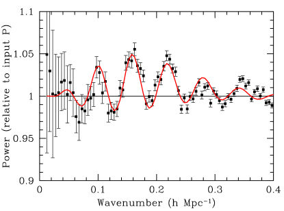
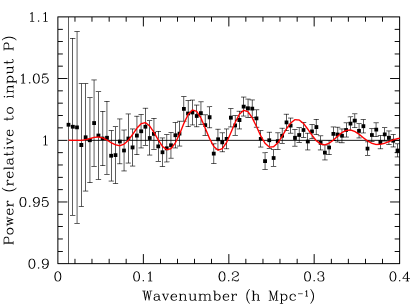
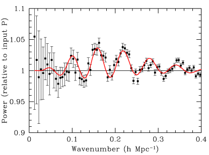
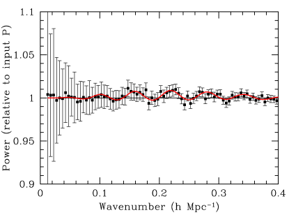
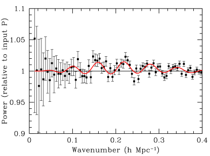
Figure 4: The power in the simulations compared to the model. The left column shows real space; the right column shows redshift space. The top row is $z=0.3$, the middle $z=1$, and the bottom row is $z=3$. In all panels, the simulation power has been fit over the range $0<k<0.4h{\rm\,Mpc}^{-1}$ to a model of $b^{2}P_{\rm smear}+a_{0}+a_{2}k^{2}+a_{4}k^{4}+a_{6}k^{6}$, where $P_{\rm smear}$ is the smeared linear power spectrum $P_{\rm linear}$, with the small scales restored by the no-wiggle form. What is plotted is the residual $P_{\rm res}=(P_{\rm measured}-a_{0}-a_{2}k^{2}-a_{4}k^{4}-a_{6}k^{6})/b^{2}$ divided by the linear power spectrum. In detail, we divide by the initial power spectrum of the simulation, so that the variations in the initial amplitudes of particular modes cancel out; this doesn’t change the sense of the plot but tightens the residuals slightly. The smeared model (red) has been similarly divided by the linear power spectrum. If the linear spectrum were fully intact, it would be flat in this plot. Erasure of the acoustic peaks produces oscillations in this plot. One sees that the model provides an excellent match to the observed degradation.

In sum, the radial displacements across and along the line of sight are well predicted by the following simple model:

$$\sigma_{\perp} = s_{0}D$$ (12)

$$\sigma_{\parallel} = s_{0}D(1+f)$$ (13)

where $D$ is the growth function and $f=d(\ln D)/d(\ln a)\approx\Omega^{0.56}$. The length $s_{0}$ is $12.4h^{-1}{\rm\,Mpc}$ for $100h^{-1}{\rm\,Mpc}$ separations in our cosmology if we normalize $D$ such that $D=(1+z)^{-1}$ at high $z$ ($D=0.758$ at $z=0$). The length will depend slightly on cosmology, at least scaling linearly with the clustering amplitude (our simulations have a linear $\sigma_{8}=0.9$ at $z=0$, but the relevant normalization scale is much above $8h^{-1}{\rm\,Mpc}$). $s_{0}$ is also a slowly increasing function of scale.

If one approximates the transverse displacements as the same, then the distribution of the displacement vector is very nearly an elliptical Gaussian, independent of the angle of the separation vector to the line of sight. To the extent that one treats $s_{0}$ as constant, the effects on the correlation function become a simple convolution, meaning that the modification of the power spectrum is simply to multiply by a Gaussian. To be clear, to the extent that the displacement distributions are Gaussians of rms $\sigma_{\parallel}$ and $\sigma_{\perp}$, along and across the line of sight, we have

$$P(\vec{k})=P_{\rm linear}(\vec{k})\exp\left(-{k_{\parallel}^{2}\over 2\sigma_{\parallel}^{2}}-{k_{\perp}^{2}\over 2\sigma_{\perp}^{2}}\right)$$ (14)

This is the model for the portion of the linear power spectrum, with acoustic peak, that survives. Of course, this is a poor model on small scales, as one has filtered out all of the small-scale clustering. One can restore the small-scale linear spectrum, without wiggles, by adding the no-wiggle approximation from Eisenstein & Hu (1998) multiplied by unity minus the smearing function.

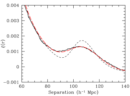
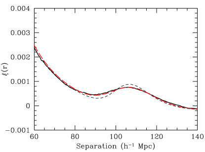
Figure 5: The correlation function in the simulations compared to the model with the small-scale linear power restored. The left panel shows $z=0.3$; the right, $z=1$. In both panels, the simulation data is the solid black line, the linear correlation function is the short-dashed thin line, and the model correlation function is the long-dashed red line. We have not removed any broad-band nuisance spectra in making this figure.

Figure 4 shows the comparison of the measured power in the simulations (Seo & Eisenstein, 2005) to the smeared model with the small-scale power restored. To make this comparison, we need to subtract off the smooth non-linear power contribution and divide out a linear bias. We do this by removing a polynomial with constant, $k^{2}$, $k^{4}$, and $k^{6}$ terms and dividing by a constant, fitting over the range $0<k<0.4h{\rm\,Mpc}^{-1}$ (Seo & Eisenstein, 2005). For redshift space, we adopt a smoothing function that is the spherical average of the elliptical Gaussian in Fourier space. In detail, we have in Figure 4 shown the power divided by the $z=49$ input power spectrum. Purely linear evolution would be a line at unity; degradations of the acoustic signature puts oscillations in the plot.

Overall the model is a very good fit. The amplitude of the oscillations in the power spectrum is well matched. The higher harmonics show more residuals, and it is not clear how much of this is a failing of the model versus noise in the power spectra. Many of the excursions at high wavenumber cannot be matched even if the acoustic oscillations are completely erased; i.e., they must be non-Gaussian noise in the simulated power spectra. However, the model assumptions to ignore the small deviations from a Gaussian distribution of displacements, the transverse displacements, and the scale dependence of the rms displacement could result in minor changes to the residuals. It is important to note that even $3.75h^{-3}{\rm\,Gpc^{3}}$ still leaves enough sample variance in the power spectrum that one cannot fully test this model at the level of 1% residuals.

Figure 5 shows the match between the correlation function in the simulation and that of the model with the small-scale power restored. Here, we do not remove any smooth power spectrum; all of these nuisance terms appear at small separations in the correlation function. Again, the agreement is good: the model seems to correctly match the smearing of the peak in the correlation function.

7 Numerical Results for Biased Tracers

Table 2:

Lagrangian Displacements Distribution for Biased Tracers
Radial Transverse $M$ $z$ $R$ Mean $\sigma$ Skewness Kurtosis $\sigma$ Kurtosis Real-space 10 0.3 100 –0.39 8.78 –0.028 0.034 7.80 0.007 30 0.3 100 –0.48 8.97 –0.026 0.024 8.02 –0.005 10 1.0 100 –0.34 6.55 –0.017 0.012 5.91 –0.028 Redshift-space 10 0.3 100 –0.65 15.00 –0.051 0.22 13.51 0.26 30 0.3 100 –0.81 15.45 –0.049 0.22 13.99 0.25 10 1.0 100 –0.64 12.93 –0.037 0.18 11.80 0.21

NOTES.—Masses of halos are listed as the number of particles $M$; each particle has a mass of $6\times 10^{11}h^{-1}\rm M_{\odot}$. Separations $R$ as well as mean and rms displacements are given in comoving $h^{-1}{\rm\,Mpc}$. Skewness and kurtosis statistics are the usual dimensionless normalization. Negative skewness means that the heavier tail is inwards. For redshift space, we list the displacements in the line-of-sight direction when this direction is radial to the initial separation vector. The displacements in the direction perpendicular to the line-of-sight are the same as in real space.

We next turn to biased tracers. We use a very simple model of bias, described in Seo & Eisenstein (2005). We find halos with a friends-of-friends algorithm (Davis et al., 1985), place a threshold on halo multiplicity, and include all of the particles in the halo as valid tracers. This is equivalent to a halo occupation model in which the number of galaxies in a halo is proportional to the halo mass, if above some threshold, and all galaxies trace the velocity dispersion of the dark matter. This is a relatively extreme model and is not intended to be realistic but simply to explore the basic effect.

Table 2 lists the moments of the Lagrangian displacement distributions for biased tracers of different mass threshold and redshift. These mass thresholds at $z=0.3$ give large-scale bias similar to that of the SDSS Luminous Red Galaxy sample (Eisenstein et al., 2001; Zehavi et al., 2005). The primary conclusion is that the bias doesn’t change the variance of the distribution much. The rms increases by 10% in real space and somewhat more in redshift space. The latter is not surprising, because the high halo masses have more small-scale thermal velocities, particularly in the bias model we use here. We interpret the small increase in real space as indicating that bulk flows affect all galaxies more or less equally, with the subdominant trend that the high mass halos have more action in their small-scale environments. It appears that bias has rather little effect on the non-linear degradation of the acoustic peaks. Figure 6 shows the power spectrum from the $z=0.3$, $M=10$ biased tracer, along with the model spectrum. As before, the agreement is excellent within the errors.

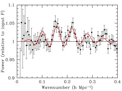
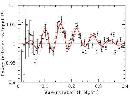
Figure 6: As Figure 4, but for a biased tracer ($M=10$) at $z=0.3$. The left panel is in real space; the right panel is in redshift space. The biased power spectrum is noisy compared to the matter power spectrum because of additional shot noise. However, one sees that the model remains a good match to the data.

However, we do find in the biased case that the mean pairwise displacements are no longer zero, as they were for the matter. The mean displacements are small, about $0.4h^{-1}{\rm\,Mpc}$ in real space for separations of $100h^{-1}{\rm\,Mpc}$, somewhat larger in redshift space. This would correspond to a 0.4% bias in the recovered distance scale, although it is not clear that this mean displacement is in fact the correct statistic to predict the exact shift. The mean for the matter displacements was zero because of homogeneity, but setting the tracer density according to the late-time matter density breaks the homogeneity assumption. We will explore this effect in detail in the next section.

8 Non-linear shifts of the acoustic scale

8.1 Spherical collapse

Until this point, we have been mostly studying how the acoustic signature is washed out by non-linear structure. This addresses the precision with which the acoustic scale can be measured in a given survey. We now turn to the question of how much non-linear collapse can actually shift the scale of the peak, so as to create a systematic bias in the measurement. In detail, the question of a shift cannot be separated from the question of what statistic or analysis one plans to use to measure the acoustic scale. That is, measuring the maximum of the peak or some centroid or performing a likelihood analysis with different templates and nuisance parameters could yield different answers when affected by nonlinearities. The choice of a measurement scheme is beyond the scope of this paper. Here we offer a discussion of the mean flows on 150 Mpc scale, which should explore the dynamics of the non-linearities.

We again begin by considering the configuration-space picture. A peak at one location creates a faint spherical echo and a preferred separation of galaxies. It is clear that the nonlinear motion caused by clusters and flows will be largely independent between the two galaxies in a given pair. In other words, most of the non-linear blurring of the peak (or erasure of the high harmonics in the power spectrum) does not shift the pairs systematically to a different separation. But it is clear that peaks in the Universe separated by $\sim\!150$ Mpc will tend to fall towards each other, and that voids will tend to move away from each other. Hence, there is a small anisotropy that could shift the acoustic scale.

How big is this effect? Let us first consider spherical collapse. If there is a matter overdensity at one point, there will tend to be a matter overdensity inside a co-centered sphere of radius $R=150{\rm\,Mpc}$. The mean value of this overdensity is related to the $J_{3}$ integral of the correlation function:

$$\left\langle\delta(<R)\right\rangle={3\delta_{0}\over R^{3}\sigma_{0}^{2}}\int_{0}^{R}dr\;r^{2}\xi(r)\equiv{3\delta_{0}\over\sigma_{0}^{2}}J_{3}(R)$$ (15)

Here, $\delta_{0}$ is the overdensity at the center, $\sigma_{0}^{2}$ is the variance in that overdensity, and $J_{3}(R)$ is the integral of the correlation function (Peebles, 1980)

$$J_{3}(s)=\int_{0}^{s}{r^{2}dr\over s^{3}}\xi(r)=\int{k^{2}dk\over 2\pi^{2}}P(k){j_{1}(ks)\over ks},$$ (16)

where $j_{1}$ is a spherical Bessel function. One can consider the density field to be smoothed, provided that the smoothing length is much smaller than $R$. Since $\delta_{0}/\sigma_{0}$ will be of order unity the mean $\delta(<R)$ will scale as $\sigma_{0}^{-1}$. If unsmoothed, then $\sigma_{0}$ is very large and the mean $\delta(<R)$ is near zero; this is simply a statement that behavior at a single point doesn’t bias an entire filled sphere very much. However, if one smoothes the density field, $\sigma_{0}$ becomes smaller. The natural smoothing scale for this problem is something similar to the width of the acoustic shell, since that is the size of the central region that adds coherently to the acoustic effect. With this smoothing, $\sigma_{0}$ is about unity at $z=0$.

The value of $3J_{3}(150{\rm\,Mpc})$ in the concordance cosmology (Spergel et al., 2006) at $z=0$ is about $0.007$, and so the mean $\delta(<R)$ is of this order. It is worth remembering that this overdensity is dominated by the correlations in the initial density field carried by the cold dark matter, not the acoustic effects. Translating the overdensity into a change in the radius of the sphere yields $\delta(<R)/3$, so the scale is changed only by $O(0.003)$. In the line-of-sight direction, redshift distortions double the apparent infall (Peebles, 1980; Kaiser, 1987) in Einstein-de Sitter, less so in low-density universes. It seems difficult to push this to be more than a 1% effect.

The rms overdensity inside a sphere of $150{\rm\,Mpc}$ radius is about 0.07 in the standard cosmology at $z=0$. However, this overestimates the infall because the small overdensities that dominate the total in the sphere can be anywhere inside the sphere, not at the center, so that the infall isn’t radial and doesn’t affect the entire spherical acoustic echo.

Thus far, we have only discussed the infall around overdensities. However, there is a equivalent outflow from underdensities. For the matter, these cancel to leading order. The next order terms do not cancel, and we therefore expect the changes in scale to be $O(10^{-4})$.

8.2 Biasing the Acoustic Scale

We next study whether applying a local galaxy bias can create a first-order motion of the acoustic scale. We wish to compute whether two galaxies separated initially by a given large distance will tend to fall toward each other. In the Zel’dovich approximation, the pair-wise displacement of two initial positions, projected along the initial separation vector, is (from eq. [8])

$$u_{12,\parallel}={\vec{u}_{12}\cdot\vec{r}_{12}\over r_{12}}=\int{d\vec{k}\over(2\pi)^{3}}\delta_{\vec{k}}{\vec{k}\cdot\vec{r}_{12}\over ik^{2}r_{12}}\left[e^{i\vec{k}\cdot\vec{r}_{1}}-e^{i\vec{k}\cdot\vec{r}_{2}}\right].$$ (17)

It is clear that $\left<u_{12,\parallel}\right>=0$; one is performing an average weighted by the initial volume, not final density, and this cancellation is required by homogeneity. If we consider $\left<u_{12,\parallel}\delta_{1}\right>$, then we find that this equal to $-r_{12}J_{3}(r_{12})$, where $J_{3}$ is defined in Equation (16). Hence, we do find that objects fall towards overdensities and away from underdensities. We note that although this is the same result as from spherical collapse, we did not assume spherical symmetry here.

We now wish to consider the mean displacement weighted by pairs, i.e.

$$u_{\parallel}^{\rm pair}\equiv{\left<u_{12,\parallel}\delta_{1}\delta_{2}\right>\over\left<\delta_{1}\delta_{2}\right>}.$$ (18)

We consider these densities to be those of the initial linear density field. The denominator $\left<\delta_{1}\delta_{2}\right>$ is simply $\xi(r_{12})$, which can be zero, but we will work in the limit where $\xi$ is small but non-zero; we find that the ratio $u_{\parallel}^{\rm pair}$ approaches a finite number as $\xi\rightarrow 0$.

In the Zel’dovich approximation, $u_{12,\parallel}$ is linear in the density field $\delta$ and hence $u_{\parallel}^{\rm pair}=0$ for a Gaussian initial density field, as the numerator is a 3-point function. The displacement field will have corrections at orders above first, but this will produce $u_{\parallel}^{\rm pair}$ at order $O[J_{3}^{2}(r_{12})]$ or worse. In other words, there is a first-order cancellation in the pair-weighted mean displacement, when one uses an unbiased tracer.

We next consider weighting by the galaxy overdensity field $\delta_{g}$. We assume a local bias model in which $\delta_{g}$ is a function simply of the initial matter density $\delta$. We write $\delta_{g,1}=\delta_{g}(\delta_{1})$. Now we have

$$u_{\parallel}^{\rm pair}\equiv{\left<u_{12,\parallel}\delta_{g,1}\delta_{g,2}\right>\over\left<\delta_{g,1}\delta_{g,2}\right>}.$$ (19)

Importantly, the displacement $u_{12,\parallel}$ still depends on the matter density field, not the galaxy density field. In the limit that $|\xi(r_{12})|$ is much smaller than the variance at a single point, $\sigma^{2}=\left<\delta_{1}^{2}\right>$, the mean Zel’dovich displacement given $\delta_{1}$ and $\delta_{2}$ is

$$\left<u_{12,\parallel}\right>_{\delta_{1},\delta_{2}}=-{r_{12}J_{3}(r_{12})\over\sigma^{2}}\left(\delta_{1}+\delta_{2}\right).$$ (20)

Keeping only the leading-order terms, we have

$$u_{\parallel}^{\rm pair}\equiv-{r_{12}J_{3}(r_{12})\over\sigma^{2}}{\left<(\delta_{1}+\delta_{2})\delta_{g,1}\delta_{g,2}\right>\over\left<\delta_{g,1}\delta_{g,2}\right>}.$$ (21)

We next consider the form of the function $\delta_{g}$. We must have $\left<\delta_{g}\right>=0$, where the averaging is over the distribution of the matter density. This simply defines the mean density of galaxies. We also have $\left<\delta_{g}\delta\right>=b\sigma^{2}$, where $\sigma^{2}=\left<\delta^{2}\right>$ and $b$ is the familiar large-scale bias. Allowing $\delta_{g}$ to be a stochastic distribution depending on the matter density at that point (e.g. Dekel & Lahav, 1999) doesn’t alter the result; to leading order, only the mean galaxy density as a function of $\delta$ enters.

To compute the expectation values, we must include the fact that $\delta_{1}$ and $\delta_{2}$ are correlated. In the limit that $|\xi(r_{12})|\ll\sigma^{2}$, we find $\left<\delta_{g,1}\delta_{g,2}\right>=b^{2}\xi(r_{12})$ and $\left<\delta_{1}\delta_{g,1}\delta_{g,2}\right>=\left[b\xi(r_{12})/\sigma^{2}\right]\left<\delta_{g,1}\delta_{1}^{2}\right>$. If we define rescaled density fields $\nu=\delta/\sigma$ and $\nu_{g}=\delta_{g}/b\sigma$, then we reach the result

$${u_{\parallel}^{\rm pair}\over r_{12}}=-{2J_{3}(r_{12})\over\sigma}\left<\nu^{2}\nu_{g}(\nu)\right>$$ (22)

where the expectation value is computed with $\nu$ being distributed as a Gaussian of unit variance. The function $\nu_{g}$ is also subject to $\left<\nu_{g}\right>=0$ and $\left<\nu_{g}\nu\right>=1$, the latter being due to the scaling by $b$.

Hence, the fractional change in the pair-weighted separation can be first order in the large-scale correlation function if the local bias is suitably chosen. However, for a linear bias, $\nu_{g}\propto\nu$ (which must actually be $\nu_{g}=\nu$), the first-order effect cancels. We remind the reader that $2J_{3}(r_{12})$ is about 0.5% for the standard cosmology at $z=0$ (and of course smaller at high redshift).

The pair-weighted mean displacement of Equation 19 is not the same as the mean displacement between pairs of tracers, as studied in § 7. The difference is effectively that of weighting by $\delta_{g}$ or by $(1+\delta_{g})/(1+\delta_{m})$. These clearly disagree on the relative weighting of overdense and underdense regions, and the tracer-based counting may fail to include the voids properly. However, in the limit of a bias model in which galaxies form only above a high density threshold, the two calculations converge to the same answer.

For a toy model inspired by Press-Schechter (1974) theory, we consider a model in which galaxy formation obeys a simple density threshold $\delta_{t}$, typically $\sim\!1.7$. For a threshold $\nu_{t}\equiv\delta_{t}/\sigma$, we find $\left<\nu^{2}\nu_{g}\right>=\nu_{t}$. This yields ${u_{\parallel}^{\rm pair}/r_{12}}=-J_{3}(r_{12})(2\nu_{t}^{2}/\delta_{t})$. The usual problems in accounting for underdense regions in Press-Schechter theory recommend that one only consider this model for reasonably extreme peaks, i.e. $\nu_{t}\gtrsim 2$. For a fixed $\delta_{t}$ and smoothing scale (and hence a rapidly declining number density of objects at higher redshift), the redshift dependence of $\nu_{t}^{2}$ and $J_{3}$ cancel, matching the behavior in Table 2. Matching the bias models used at $z=0.3$ in § 7 would suggest $\nu_{t}\approx 1.6$, which makes $u_{\parallel}^{\rm pair}/r_{12}\sim-0.6\%$, somewhat larger than the measured mean displacement but in qualitative agreement. However, it is not surprising that the actual halo bias is closer to linear than the sharp threshold model.

Estimating an exact level of the bias in the measured acoustic scale is not straight-forward from this local bias formalism, as one has to decide what smoothing scale to apply to the initial density field, both to define the local bias model $\nu_{g}(\nu)$ and to compute the matter variance $\sigma^{2}$. One sees, however, that one is caught between two limits in which the cancellation is restored: if one chooses a large smoothing scale, then $\sigma$ can be small, but the local bias becomes more linear, whereas with a small smoothing scale, the bias will be non-linear, but $\sigma$ is larger. Hence, it seems likely that the combination $\left<\nu^{2}\nu_{g}\right>\sigma^{-1}$ will be somewhat less than 1 at $z=0$, yielding a shift of about 0.5%. The shift in the acoustic scale should decrease at high redshift, somewhat slower than the square of the growth function, for tracers of a given number density.

To summarize, for objects that trace the matter, the inflow between positive density pairs exactly cancels the outflow between negative density pairs. Galaxy bias can shift the balance, yielding a net flow. Fortunately, the effect involved, namely the flows on 150 Mpc scale is very easy to simulate. We expect that large volume gravitational simulations with relatively poor mass resolution should be able to give accurate estimates of the effect for various galaxy bias prescriptions.

9 Conclusions

We have investigated the non-linear degradation of the baryon acoustic signature through several different methods. We argue that as the clustering signature is manifested as a peak in the correlation function on large scales, the degradation enters primarily through the motion of the two galaxies altering the separation between them. This smearing is due to small-scale thermal motion, e.g., cluster formation, and coherent motions, e.g., bulk flows into superclusters or out of voids between the two objects. This smearing broadens the peak in the correlation function and decreases the higher harmonics in the power spectrum.

We model this smearing by measuring the distribution of differences of the Lagrangian displacements of pairs of particles initially separated by a separation equal to the sound horizon. These distributions are close to Gaussian in both real and redshift space, and we find that the redshift dependence of the rms width is well predicted by the linear-theory scaling predictions. We propose convolving the linear theory correlation function with this Gaussian. The linear theory power spectrum can be multiplied by the Fourier transform of this Gaussian, and the small-scale power restored using the no-wiggle form from Eisenstein & Hu (1998).

This model has significant advantages. First, the displacements can be calculated with a relatively modest volume of cosmological simulations compared with those required to measure the degraded power spectrum. However, one should use box sizes of at least $512h^{-1}{\rm\,Mpc}$ to model the required wavelengths. Second, the Lagrangian displacements are easy to calculate in real or redshift space and can be applied to arbitrary tracers of the field, as the fuzzy nature of the initial position of a galaxy is still well confined relative to the width of the Lagrangian displacement distribution. Third, in the context of survey parameter estimation, one can now avoid the assumption of simply truncating the linear mode counting at a given maximum wavenumber, as has been the standard practice (e.g., Eisenstein, Hu, & Tegmark, 1998; Seo & Eisenstein, 2003, among many others). Instead, we now have an accurate model for the quasi-linear acoustic signature, in which the higher harmonics are gradually erased. We plan to include this model in survey forecasts in a future paper.

Although degradations of the acoustic signature are important to estimating the statistical performance of a given volume, an actual shift in the acoustic scale would be more important, as this would lead to a bias in the inferred distance scale. The idea that the acoustic signature is a single peak in the correlation function allows one to argue that these effects must be small: to shift the peak, one must systematically move pairs initially at $150{\rm\,Mpc}$ scale outward or inward on average. We have investigated this with two different models, the mean pairwise displacement of tracers and the pair-weighted mean displacement in the Zel’dovich approximation. In both cases, we find that linearly biased tracers imply a cancellation of the first-order terms, which would make the shift negligible at $O(10^{-4})$. With biased galaxy formation, we estimate shifts of order 0.5% for objects with $b\approx 2$ at $z=0$, dropping at higher redshift. However, neither of our models are exact, nor have we considered the issue of how a particular choice of statistic by which one measures the acoustic scale might be affected by non-linearities. We believe that large volumes of simulations will be needed to refine the estimates and calibrate particular measurement techniques. It is highly plausible that corrections could be derived from simulations that would decrease the residual shift by a factor of a few and reach $10^{-3}$ accuracy. After all, any survey capable of reach statistical precision on the acoustic scale at levels of 0.5% or better will have fantastic data on the small-scale clustering and environments of the tracer galaxies.

By viewing the non-linear acoustic signature as the spreading of a preferred separation, one sees that the acoustic scale must be robust to the effects of scale-dependent bias and non-linear clustering. This is not obvious in the power spectrum, where the higher acoustic harmonics ($k\approx 0.2h{\rm\,Mpc}^{-1}$) appear at the same wavenumber as the quasi-linear regime. The key point is that the peaks and troughs of the acoustic series define a beat frequency that is at very large wavelength. Alternatively stated, non-linearities on $10h^{-1}{\rm\,Mpc}$ scales can only introduce broad-band ($\Delta k\approx 0.1h{\rm\,Mpc}^{-1}$) modifications of the power spectrum and therefore cannot affect the peaks and troughs differentially, save to damp out the entire linear spectrum.

The fact that small-scale non-linear clustering produces smooth power spectra compared to the acoustic oscillations is also important for making unbiased measurements of the acoustic scale. The measured power spectra will generally be tilted relative to the linear spectrum, and it is well-known that when measuring the position of a peak, one must avoid tilting the baseline on which the peak sits. This leads to the speculation that non-linearities can bias the measurement of the acoustic scale. We see here that this need not be the case. In configuration space, these effects collapse to small separations, well-separated from the acoustic scale. Alternatively, in Fourier space, one can marginalize over smooth nuisance functions. The linear power spectrum predicted as part of the sound horizon calculation provides an easy template against which to make an unbiased measurement.

In short, the acoustic scale is a robust standard ruler because it is fundamentally a $150{\rm\,Mpc}$ clustering signature. This is far larger than the characteristic scales for halo formation and galaxy bias, and the 10% width of the peak makes it very implausible to mimic by astrophysical processes. We have shown here that the degradations of the signature have benign quasi-linear causes. These can be computed to high accuracy with N-body gravitational simulations. The remaining challenge for the method is the enormous survey volumes required to measure the scale to high precision.

DJE thanks Michael Joyce for useful conversations and the Miller Institute at the University of California for support during a key period in the development of this paper. DJE and HS are supported by grant AST-0407200 from the National Science Foundation. DJE is further supported by an Alfred P. Sloan Research Fellowship. M.W. is supported by NASA and the NSF.

Appendix A An Investigation of Local Bias

In the configuration-space picture of the acoustic signature, the sound waves created by a peak in the density field leave a small residual overdensity in a shell at $150{\rm\,Mpc}$ radius. We consider in this appendix whether there is a judicious choice of tracers that would increase the contrast of the shell or peak, so as to increase the strength of the signature in the correlation function. Unfortunately, we will conclude that there is not, reinforcing the concepts of linear bias.

The thickness of this shell is about $10{\rm\,Mpc}$ because of Silk damping and the damping of oscillatory modes. Hence, two points separated by $\ll 10{\rm\,Mpc}$ create acoustic shells that essentially overlap. In what follows, we consider the density field smoothed on $10{\rm\,Mpc}$ scales.

The variance at low redshift in the overdensity in $10{\rm\,Mpc}$ patches is roughly unity. The corresponding echos at $150{\rm\,Mpc}$ separation are only 1% in amplitude, far smaller than the primary variations at those locations (which are again order unity). The smallness of the echo suggests that a local bias model should apply. We therefore consider the response of the behavior in $10{\rm\,Mpc}$ patches when acted upon by bulk shifts in their density, corresponding to long-wavelength perturbations.

We will consider two regions of size $\sim\!10{\rm\,Mpc}$ separated by a distance of $150{\rm\,Mpc}$. We write the linear matter overdensity (ignoring the acoustic effect) in the two as $\delta_{m,1}$ and $\delta_{m,2}$; The $\delta_{m}$ will be Gaussian distributed with variance $\sigma$; we write the distribution as $p(\delta_{m})$. Because of the acoustic effect, the density at location 2 will actually be $\delta_{m,2}+\alpha\delta_{m,1}$, where $\alpha$ is about 0.01. There is a recipricol effect on the density at location 1 which we ignore for clarity.

Now we imagine that galaxies are formed in a region of density $\delta_{m}$ with a mean density of $\rho_{g}(\delta_{m})$. Of course, the actual number will scatter from the mean, but only the mean enters this calculation. The homogeneous density of galaxies is $\bar{\rho}_{g}=\int d\delta_{m}\;p(\delta_{m})\rho_{g}(\delta_{m})$. We define the galaxy overdensity as $\delta_{g}(\delta_{m})=[\rho_{g}(\delta_{m})-\bar{\rho}]/\bar{\rho}$.

With such a model, the bias at large scales (small wavenumber) should be the response of this density to a small long-wavelength fluctuation in the matter density:

$$b=\lim_{\epsilon\rightarrow 0}{\int d\delta_{m}\;p(\delta_{m})\rho_{g}(\delta_{m}+\epsilon)-\bar{\rho}\over\epsilon\bar{\rho}}={\int d\delta_{m}\;p(\delta_{m})\delta_{g}(\delta_{m}+\epsilon)\over\epsilon}=\int d\delta_{m}\;p(\delta_{m}){d\delta_{g}\over d\delta_{m}}.$$ (A1)

Meanwhile, the amplitude of the acoustic effect should be the product of the galaxy overdensities at the two locations:

$$B^{2}=\int d\delta_{m,1}\;p(\delta_{m,1})\delta_{g}(\delta_{m,1})\int d\delta_{m,2}\;p(\delta_{m,2})\delta_{g}(\delta_{m,2}+\alpha\delta_{m,1})$$ (A2)

Because $\alpha$ is small, we can use the limit in equation (A1) to form

$$B^{2}=\int d\delta_{m,1}\;p(\delta_{m,1})\delta_{g}(\delta_{m,1})b\alpha\delta_{m,1}.$$ (A3)

One might at this point have thought that by picking $\delta_{g}$ judiciously one could produce an amplitude for the acoustic peak that would increase its contrast relative to the square of the large-scale bias. In other words, one has a large peak in region 1 and a faint echo in region 2. The galaxy density in region 2 is unavoidably controlled by the standard large-scale bias, as the acoustic signature is a subdominant echo at that location. But one could hope that one could pick a tracer that would emphasize region 1 more. One could even imagine cross-correlating two tracer sets, one that maximizes signal-to-noise for small long-wavelength perturbations (region 2) and the other that picks out high peaks (region 1).

Unfortunately, this is all for naught. Integrating equation (A3) by parts yields

$$B^{2}=\alpha b^{2}\sigma^{2}$$ (A4)

for any $\rho_{g}(\delta_{m})$ bias function. The trick is that the indefinite integral of $\delta_{m}p(\delta_{m})$ is just $-\sigma^{2}p(\delta_{m})$ because the initial density distribution $p$ is a Gaussian.

This result shows that at the level of local bias, one cannot pick the tracer to maximize the contrast in the acoustic peak in the linear regime. This is a simple corollary of the usual theorems about local bias (Coles, 1993; Scherrer & Weinberg, 1998). It may be possible to find tracers that minimize the non-linear spreading of the acoustic peak or that minimize the amount of small-scale near-white noise; such tracers would improve the signal-to-noise ratio of the measurement. But there is no opportunity at the simple level of pair counting.

References

- Amendola et al. (2005) Amendola, L., Quercellini, C., & Giallongo, E., 2005, MNRAS, 357, 429
- Bashinsky & Bertschinger (2001) Bashinsky, S., & Bertschinger, E., 2001, Phys. Rev. Lett., 87, 1301
- Bashinsky & Bertschinger (2002) Bashinsky, S., & Bertschinger, E., 2002, Phys. Rev. D, 65, 3008
- Bennett, Turner, & White (1997) Bennett C., Turner M., White M., 1997, Physics Today, 50, 32
- Bennett et al. (2003) Bennett, C., et al., 2003, ApJS, 148, 1
- Blake & Glazebrook (2003) Blake, C., & Glazebrook, K., 2003, ApJ, 594, 665
- Blake & Bridle (2005) Blake, C., & Bridle, S., 2005, MNRAS, 363, 1329
- Blake et al. (2006) Blake, C., Parkinson, D., Bassett, B., Glazebrook, K., Kunz, M., & Nichol, R.C., 2006, MNRAS, 365, 255
- Blumenthal et al. (1984) Blumenthal G.R., Faber S.M., Primack J.R., Rees M.J., 1984, Nature, 311, 517
- Bond & Efstathiou (1984) Bond, J.R. & Efstathiou, G. 1984, ApJ, 285, L45
- Cole et al. (2005) Cole, S., et al., 2005, MNRAS, 362, 505
- Coles (1993) Coles, P. 1993, MNRAS, 262, 1065
- Cooray, Hu, Huterer & Joffre (2001) Cooray A., Hu W., Huterer D., Joffre M., 2001, ApJ, 557, L7
- Crocce & Scoccimarro (2005) Crocce, M., & Scoccimarro, R., 2005, astro-ph/0509419
- Davis et al. (1985) Davis M., Efstathiou G., Frenk C.S., White S.D.M., 1985, ApJ, 292, 371
- de Bernardis et al. (2000) de Bernardis, P., et al., 2000, Nature, 404, 995
- Dekel & Lahav (1999) Dekel, A., & Lahav, O., 1999, ApJ, 520, 24
- Dolney, Jain, & Takada (2006) Dolney, D., Jain, B., & Takada, M., 2006, MNRAS, 366, 844
- Doroshkevich, Zel’dovich, & Sunyaev (1978) Doroshkevich, A.G., Zel’dovich, Ya.-B, Sunyaev, R.A., 1978, Soviet Astronomy, 22, 523
- Eisenstein & Hu (1998) Eisenstein, D.J., & Hu, W. 1998, ApJ, 496, 605
- Eisenstein, Hu, & Tegmark (1998) Eisenstein, D. J., Hu, W., & Tegmark, M. 1998, ApJ, 504, L57
- Eisenstein et al. (2001) Eisenstein, D.J., Annis, J., Gunn, J.E., Szalay, A.S., Connolly, A.J., Nichol, R.C., et al., 2001, AJ, 122, 2267
- Eisenstein (2003) Eisenstein, D.J., 2003, in Wide-field Multi-Object Spectroscopy, ASP Conference Series, ed. A. Dey
- Eisenstein et al. (2005) Eisenstein, D.J., et al., 2005, ApJ, 633, 560
- Glazebrook & Blake (2005) Glazebrook, K., & Blake, C., 2005, ApJ, 631, 1
- Goroff et al. (1986) Goroff, M.H., Grinstein, B., Rey, S.-J., & Wise, M.B., 1986, ApJ, 311, 6
- Groth & Peebles (1975) Groth E.J., Peebles P.J.E., 1975, Astron. & Astrophys., 41, 143
- Gurbatov et al. (1989) Gurbatov, S.N., Saichev, A.I., & Shandarin, S.F., 1989, MNRAS, 236, 385
- Halverson et al. (2002) Halverson, N.W., et al., 2002, ApJ, 568, 38
- Hamilton (1998) Hamilton, A.J.S., 1998, “The Evolving Universe”, ed. Hamilton (Kluwer Academic), p. 185; astro-ph/9708102
- Hanany et al. (2000) Hanany, S., et al., 2000, ApJ, 545, L5
- Hu & Sugiyama (1995) Hu W., Sugiyama N., 1995, ApJ, 444, 489
- Hu & White (1996) Hu, W., & White, M., 1996, ApJ, 471, 30
- Hu & White (1997) Hu W., White M., 1997, ApJ, 479, 568
- Hu et al. (1997) Hu, W., Sugiyama, N., & Silk, J. 1997, Nature, 386, 37
- Hu & Dodelson (2002) Hu, W., & Dodelson, S., 2002, ARA&A, 40, 171
- Hu & Haiman (2003) Hu, W. & Haiman, Z., 2003, Phys. Rev. D, 68, 3004
- Jain & Bertschinger (1994) Jain, B., & Bertschinger, E., 1994, ApJ, 431, 495
- Jeong & Komatsu (2006) Jeong, D., & Komatsu, E., 2006, ApJ, submitted
- Kaiser (1987) Kaiser, N., 1987, MNRAS, 227, 1
- Kodama & Sasaki (1984) Kodama, H., Sasaki M., 1984, Prog. Theor. Phys., 78, 1
- Kofman & Shandarin (1988) Kofman, L.A., & Shandarin, S.F., 1988, Nature, 334, 129
- Lifshitz (1946) Lifshitz E.M., 1946, J.Phys. USSR, 10, 116.
- Linder (2003) Linder, E.V., 2003, Phys. Rev. D, 68, 3504
- Matsubara (2004) Matsubara, T., 2004, ApJ, 615, 573
- Matsubara et al. (2004) Matsubara, T., Szalay, A.S., & Pope, A.C., 2004, ApJ, 606, 1
- Meiksin et al. (1999) Meiksin, A., White, M., & Peacock, J. A. 1999, MNRAS, 304, 851
- Miller et al. (1999) Miller, A.D., et al., 1999, ApJ, 524, L1
- Netterfield et al. (2002) Netterfield, C.B., et al., 2002, ApJ, 571, 604
- Padmanabhan (1993) Padmanabhan T., 1993, “Structure formation in the Universe”, Cambridge University Press, Cambridge.
- Peebles (1968) Peebles, P. J. E., 1968, ApJ, 153, 1
- Peebles & Yu (1970) Peebles, P. J. E. & Yu, J. T. 1970, ApJ, 162, 815
- Peebles (1980) Peebles, P.J.E., 1980, The Large-Scale Structure of the Universe (Princeton: Princeton Univ. Press)
- Peebles (1981) Peebles, P. J. E., 1981, ApJ, 248, 885
- Press & Schechter (1974) Press, W.H., & Schechter, P., 1974, ApJ, 187, 425
- Press & Vishniac (1980) Press W.H., Vishniac E.T., 1980, ApJ, 236, 323
- Scherrer & Weinberg (1998) Scherrer, R.J., & Weinberg, D.H. 1998, ApJ, 504, 607
- Schulz & White (2006) Schulz, A.E., & White, M., 2006, Astropart. Phys, 25, 172
- Scoccimarro (2004) Scoccimarro, R., 2004, Phys. Rev. D, 70, 3007
- Seager, Sasselov, & Scott (1999) Seager S., Sasselov D., Scott D., 1999, ApJ, 523, L1
- Seljak & Zaldarriaga (1996) Seljak, U., & Zaldarriaga, M., 1996, ApJ, 469, 437
- Seo & Eisenstein (2003) Seo, H., & Eisenstein, D.J., 2003, ApJ, 598, 720
- Seo & Eisenstein (2005) Seo, H., & Eisenstein, D.J., 2005, ApJ, 633, 575
- Silk (1968) Silk, J., 1968, ApJ, 151, 459
- Spergel et al. (2006) Spergel, D.N., et al., 2006, submitted
- Springel et al. (2005) Springel, V., et al., 2005, Nature, 435, 629
- Steigman (2006) Steigman, G., 2006, Int. J. Mod. Phys., E15, 1
- Sunyaev & Zel’dovich (1970) Sunyaev, R.A., & Zel’dovich, Ya.B., 1970, Ap&SS, 7, 3
- White (2005) White M., 2005, Astropart. Phys., 24, 334
- White & Cohn (2002) White M., Cohn J.D., 2002, Am.J.Phys., 70, 106
- Wilson & Silk (1981) Wilson M.L., Silk J., 1981, ApJ, 243, 14
- Zaldarriaga & Seljak (2000) Zaldarriage, M., & Seljak, U., 2000, ApJS, 129, 431
- Zehavi et al. (2005) Zehavi, I., et al., 2005, ApJ, 621, 22
- Zel’dovich (1970) Zel’dovich, Y.A., 1970, A&A, 5, 84
- Zel’dovich, Kurt, & Sunyaev (1969) Zel’dovich, Ya-B., Kurt V.G., Sunyaev R.A., 1969, Sov. Phys. JETP, 28, 146