The QUEST RR Lyrae Survey II: The Halo Overdensities in the First Catalog

Abstract

The first catalog of the RR Lyrae stars (RRLS) in the Galactic halo by the Quasar Equatorial Survey Team (QUEST) has been searched for significant overdensities that may be debris from disrupted dwarf galaxies or globular clusters. These RRLS are contained in a band $\sim 2\fdg 3$ wide in declination that spans $\sim 165\arcdeg$ in right ascension and lie $\sim 4$ to $\sim 60$ kpc from the Sun. Away from the major overdensities, the distribution of these stars is adequately fit by a smooth halo model, in which the flattening of the halo decreases with increasing galactocentric distance (Preston et al., 1991). This model was used to estimate the “background” of RRLS on which the halo overdensities are overlaid. A procedure was developed for recognizing groups of stars that constitute significant overdensities with respect to this background. To test this procedure, a Monte Carlo routine was used to make artificial RRLS surveys that follow the smooth halo model, but with Poisson distributed noise in the numbers of RRLS and, within limits, random variations in the positions and magnitudes of the artificial stars. The $10^{4}$ artificial surveys created by this routine were examined for significant groups in exactly the same way as the QUEST survey. These calculations provided estimates of the frequencies with which random fluctuations produce significant groups.

In the QUEST survey, there are six significant overdensities that contain six or more stars and several smaller ones. The small ones and possibly one or two of the larger ones may be artifacts of statistical fluctuations, and they need to be confirmed by measurements of radial velocity and/or proper motion. The most prominent groups are the northern stream from the Sagittarius dwarf spheroidal galaxy and a large group in Virgo, formerly known as the “12.4 hr clump”, which recently Duffau et al. (2006) have shown contains a stellar stream (the Virgo Stellar Stream). Two other groups lie in the direction of the Monoceros stream and at approximately the right distance for membership. Another group is related to the globular cluster Palomar 5.

1 INTRODUCTION

Recent surveys of the galactic halo have shown that it contains streams of stars emanating from dwarf galaxies. The firmest evidence for this comes from the numerous detections of streams from the Sagittarius (Sgr) dwarf spheroidal galaxy (hereafter dSph), which wrap around the sky (Majewski et al., 2003). There is also strong evidence for another large stream, the Monoceros Stream (Newberg et al., 2002; Yanny et al., 2003), that forms a ring-like structure around the Milky Way (Ibata et al., 2003). Several authors have argued that the parent galaxy of the Mon Stream lies in the constellation Canis Major, but there is considerable controversy over this association and even the existence of the CMa galaxy (Martin et al., 2004; Momany et al., 2004; Martínez-Delgado et al., 2005; Carraro et al., 2005; Peñarrubia et al., 2005, among others). These on-going merger events may be only the most recent examples of a long history of mergers that build the Milky Way from an ensemble of smaller systems, as proposed by hierarchical picture of galaxy formation (e.g. Bullock & Johnston, 2005). While the evidence for ancient merger events are less spectacular than that for the recent ones, it is nonetheless compelling. It has long been speculated that the thick disk was produced by a merger of the Milky Way with a relatively large satellite galaxy soon after the formation of the first disk structure (see review by Freeman & Bland-Hawthorn, 2002). Although the very unusual globular cluster $\omega$Cen has not yet been directly linked to a merger event, its exceptional structure and internal ranges in metallicity and in age has fueled speculation that it is the nucleus of a now extinct nucleated dwarf galaxy (Carraro & Lia, 2000; Tsuchiya et al., 2003; Ideta & Makino, 2004; Rey et al., 2004, among others).

Simulations of the destruction of dwarf galaxies (Johnston et al., 1996; Harding et al., 2001) have shown that the tidal debris may be recognized in the halo as over-densities in space and as coherent structures in radial velocity space long after the merger event. By detecting this debris, modeling their orbits, and studying their ages and chemical compositions, the merger history of the Milky Way may be pieced together. In addition to documenting the importance of mergers to galactic evolution, this may help explain the large inconsistency between the number of satellite galaxies predicted by the hierarchical picture for the formation of a large galaxy and the relatively small number of satellite galaxies around the Milky Way, the ”satellite problem” (see Freeman & Bland-Hawthorn, 2002).

Debris from satellite galaxies is not the only kind expected in the galactic halo. Numerical simulations have shown that several processes can lead to the disruption of globular clusters, and there has been much speculation that the roughly 150 the globular clusters that are now identified in the Galaxy are the survivors of a once much larger population (e.g. Gnedin & Ostriker, 1997). A few examples of tidal tails from globular clusters have been reported (Grillmair et al., 1995; Leon et al., 2000), the most spectacular of which are the streams that stretch several degrees from the globular cluster Pal 5 (Odenkirchen et al., 2001, 2003). Kinman et al. (2004) have detected some small groups of RR Lyrae variables that have similar radial velocities and metallicities, precisely the properties expected of debris from disrupted globular clusters.

In this paper we discuss the spatial distribution of the stars that were discovered in the first band of the QUEST RR Lyrae Survey (Vivas et al., 2004). RR Lyrae stars (hereafter RRLS) were selected for this survey of halo substructure because they are easily detected and are excellent standard candles. Our primary goal is to identify overdensities that may be debris from dwarf galaxies or from globular clusters. In a few structures identified here, the densities of the RRLS are so much higher than the average densities of variables that there is little doubt that the feature is real and not a random fluctuation in the background. Not all of the other features identified here may be real, and they require confirmation by determining if their member stars have similar motions. We will report in later papers our measurements of the radial velocities and the metallicities of the stars in some of these spatial groups.

2 THE POPULATION BIAS OF A RRLS SURVEY

Before discussing the QUEST survey, it is import to consider a bias that affects all RRLS surveys. RRLS are only found in the oldest (age $\geq 9$ Gyrs) stellar populations that have the proper combination of [Fe/H] and other factors (“2nd parameters” e.g., age, CNO/Fe, He/H, and stellar density) to enable horizontal branch (HB) stars to evolve into the instability strip. These complexities of HB morphology produce a wide range of RRLS populations even among the outwardly similar old and metal-poor globular clusters in the Galactic halo. Some of these clusters contain several tens of RRLS, others contain only a few RRLS, and some contain none at all. Clearly a search for the debris from destroyed globular clusters is limited by this effect, but does it also seriously impact a search for stellar streams from dwarf galaxies?

The RRLS populations in globular clusters has been quantified by Suntzeff et al. (1991), who following Kukarkin (1973), calculated the specific frequency of RRLS which they defined as the number of RRLS per unit absolute visual magnitude ($M_{V}$), normalized to $M_{V}=-7.5$ (we call this $S_{RR}$ following the 2003 version of the Harris (1996) catalogue). This fiducial $M_{V}$ is near the peak of the distribution of the Milky Way globular clusters. Using measurements of $S_{RR}$ for a large sample of globular clusters, Suntzeff et al. (1991) demonstrated that there is a systematic variation in the frequencies of RRLS with Galactocentric distance ($R_{gal}$) in the sense that the metal-poor globular clusters in the outer halo ($R_{gal}>R_{0}$) have higher frequencies than do inner halo clusters of the same metallicity. This effect, which is due to the variation of the 2nd parameter with $R_{gal}$ (e.g. Searle & Zinn, 1978) may explain the difference in mean metallicity between the field RRLS lying in the inner and outer halos (Suntzeff et al., 1991; Zinn, 1986).

We are interested here in examining $S_{RR}$ in low-mass dwarf galaxies as well as in globular clusters. The dSph galaxies provide a convenient sample of dwarf galaxies covering the extreme low-mass range of the distribution of galaxies. Because they are the most numerous type of satellite galaxy around the Milky Way and M31, it is likely that dSph galaxies were the type most frequently destroyed in the past. The Sgr dSph galaxy is of course undergoing tidal destruction at the present time. Values of $S_{RR}$ for 9 of the 10 known dSph companions of the Milky Way and for 4 of the 7 dSph companions of M31 have been computed and are listed in Table The QUEST RR Lyrae Survey II: The Halo Overdensities in the First Catalog (insufficient data were available for the other dSph companions). With two exceptions, the values of $M_{V}$ in this table were taken from Irwin & Hatzidimitriou (1995) and McConnachie & Irwin (2006) for the Milky Way and the And systems, respectively. Odenkirchen et al. (2001) have shown that Draco has a significantly larger radius than was previously measured. To estimate the $M_{V}$ of Draco, we adopted $(V-I_{C})_{0}=0.9$ for its integrated color, which is consistent with its old and very metal-poor stellar population. With the transformation equation in Odenkirchen et al. (2001), this value yields $(V-i)_{0}=0.4$, which we added to the value of $M_{i}=-8.77\pm 0.2$ (Odenkirchen et al., 2001). For the Sgr dSph, we adopted the $M_{V}$ that Cseresnjes (2001) derived, which lies in near the middle of the range quoted in the recent literature. The values of the mean [Fe/H] of the galaxies were taken from Mateo (1998) for the Milky Way companions and from Pritzl et al. (2002, 2004, 2005) for the And galaxies. Because dSph galaxies have significant internal dispersions in [Fe/H] and because the RRLS are among the oldest stars, the mean [Fe/H] of a galaxy may be larger than the mean value of its RRLS. The important point for our discussion is that the RRLS in these systems probably span a range in [Fe/H] that is not grossly different from the range observed among the RRLS in the outer Galactic halo (Suntzeff et al., 1991, $-0.9>\rm{[Fe/H]}>-2.5$). It is possible then that the field RRLS formed in similar galaxies that were later torn apart. In Table The QUEST RR Lyrae Survey II: The Halo Overdensities in the First Catalog, $N_{obs}$ is the number of RRLS that were observed in the fields covered in the variability searches, and $N_{est}$ is our estimate of the total number of RRLS in the galaxies. For most of the galaxies, we calculated $N_{est}$ from $N_{obs}$ by dividing $N_{obs}$ by the fraction of total galaxy light that is included in the observed field. For the Milky Way systems, we computed these fractions from King (1962) profiles, using the parameters given by Irwin & Hatzidimitriou (1995). The ellipticities of the galaxies were taken into account, and it was assumed that the observed fields coincided with the centers of the systems. Pritzl et al. (2002, 2004, 2005) estimated the fractions of the luminosities of the And galaxies that were covered by their fields, which made the calculations of $N_{est}$ straightforward. For the Sgr dSph galaxy, we adopted the estimate by Cseresnjes (2001) that its main body contains 4200 type ab variables. We then used the observed ratio of the type c to type ab RRLS to derive $N_{est}$. For Draco, we set $N_{est}=N_{obs}$ because Kinemuchi et al. (2002) did not specify the size of their field. Draco is so rich in variables that it matters little to our discussion that this procedure may have underestimated its $S_{RR}$. The standard deviations ($\sigma$) of the values of $S_{RR}$ were calculated by assuming Poisson statistics applies to $N_{est}$ and by adopting the uncertainties in $M_{V}$ given by their sources. Because the $N_{est}$ values are only estimates, the $\sigma$’s listed in Table The QUEST RR Lyrae Survey II: The Halo Overdensities in the First Catalog should be treated as lower limits. The variability studies probably missed some variables, and consequently, the values of $S_{RR}$ in Table The QUEST RR Lyrae Survey II: The Halo Overdensities in the First Catalog are more likely to be too small than too large. This is particularly true for the Fornax galaxy because Bersier & Wood (2002) state there are other variable stars of the right magnitude to be RRLS for which they could not determine periods.

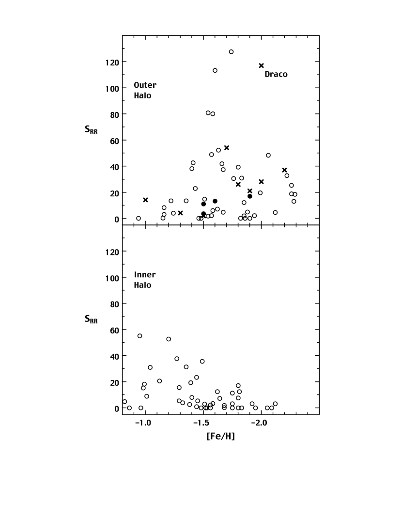
Figure 1: For halo globular clusters (open circles) and dSph companions of the Milky Way ($\times$’s) and Andromeda (solid points), the specfic frequency of RRLS ($S_{RR}$) is plotted against [Fe/H]. The upper and lower diagrams are the plots for the outer ($R_{gal}>R_{0}$) and inner ($R_{gal}<R_{0}$) halo, respectively. All of the Milky Way dSph companions lie in the outer halo, where we have also plotted the And galaxies for comparison.

In Figure 1, $S_{RR}$ for the globular clusters (Harris 2003 catalogue) and the dSph galaxies are compared. One can see again the difference in $S_{RR}$ among the metal-poor globular clusters in the inner and outer halos. The near zero values of $S_{RR}$ among the metal-poor clusters of the inner halo suggest that RRLS may not be a good tracer of its stellar populations. RRLS may be better probes of the outer halo, where the mean value of $S_{RR}$ for the clusters is well above zero. The dSph galaxies span a wide range in $S_{RR}$, but none has $S_{RR}=0$. Draco has a remarkably high value that is comparable to the highest values in the sample of 90 globular clusters. Several of the other dSph galaxies have values of $S_{RR}$ that are comparable to the variable-rich outer halo clusters. This is somewhat remarkable because many of these galaxies contain substantial populations of intermediate-aged stars that contribute to the total luminosities of the galaxies but not of course to the samples of RRLS.

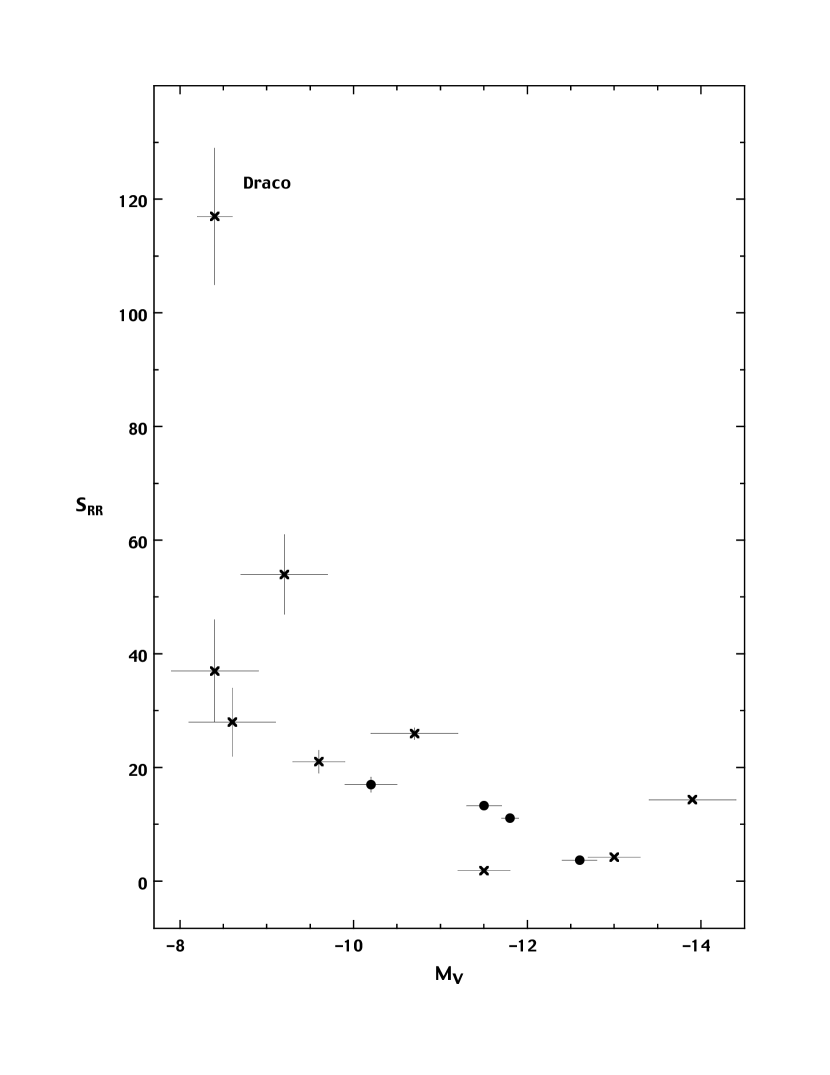
Figure 2: The specific frequencies ($S_{RR}$) of the RRLS in dSph galaxies is plotted against their absolute visual magnitudes ($M_{V}$). The $\times$’s and solid points depict the Milky Way and Andromeda companions, respectively.

$S_{RR}$ is plotted against $M_{V}$ for the galaxies in Figure 2, where one can see a clear trend of decreasing $S_{RR}$ with increasing galaxy luminosity. This is not surprising because the more luminous galaxies tend to have larger populations of intermediate-age stars. Note that the Milky Way and And galaxies are indistinguishable in this plot. The small but still significantly above zero values of $S_{RR}$ among the high luminosity galaxies indicate that their destruction will release large numbers of RRLS. It is not surprising then that the tidal streams from the Sgr dSph galaxy have been easily detected by RRLS surveys (see below and also Ivezić et al., 2000). The higher $S_{RR}$ among the low luminosity dSph galaxies partially offsets the greater difficulty that any probe of the halo will have detecting the smaller streams that are produced by the tidal destruction of low-luminosity systems.

If the 13 galaxies in Table The QUEST RR Lyrae Survey II: The Halo Overdensities in the First Catalog are representative of the dwarf galaxies that merged with the Milky Way, then RRLS surveys for stellar streams are probably not seriously handicapped by the population bias. They may also detect the debris from the destruction of the most luminous and variable rich globular clusters. Because RRLS are superior standard candles (see below), RRLS surveys may provide a better description of halo substructure than other surveys that employ probes that suffer less from population biases (e.g., K giants).

3 THE QUEST RR LYRAE SURVEY

The first band of the QUEST RR Lyrae survey (Vivas et al., 2004, hereafter Paper I) identified 498 RRLS in almost 380 deg² of the sky that spans a wide range of galactic coordinates and in apparent magnitude ($13.7<V<19.7$). Paper I describes in detail the techniques of the survey and its completeness. The survey covered a $2\fdg 3$ wide strip of the sky, centered at declination $\delta=-1^{\circ}10\farcm 8$, from right ascencion ($\alpha$) $4\fh 1$ to $6\fh 1$ and from $8\fh 0$ to $17\fh 0$. The span from $6\fh 1$ to $8\fh 0$ was not observed because it includes regions near the galactic plane. Subsequent work on the individual stars in the catalogue has shown that 41 of them are not real variables. Their apparent variability was produced in most cases by close neighbors not resolved by the QUEST instrumentation. The photometric pipeline that was used did not include a deblending algorithm. The regions most affected by blends were the ones closest to the galactic plane which present the most crowding. These regions were also the less observed in the QUEST survey and consequently there is a small number of observations per star. With few epochs available there was a greater chance that the variations in magnitude that were produced by the poor centering on a blended image mimicked a RRLS light curve. Only 3 cases of blends were found at high galactic latitudes ($9\fh 1<\alpha<16\fh 0$), which represents only the $0.8\%$ of all the stars in the catalogue in that region.We eliminated all cases of blends before preforming the following analysis on the remaining 457 RRLS.

4 THE DISTANCES OF THE RRLS

The distances of the RRLS from the Sun ($r_{\sun}$) are estimated in the usual way from measurements of their mean V magnitudes, $\langle V\rangle$, and interstellar extinctions, $A_{V}$, and by assuming an average value for their absolute magnitudes, $M_{V}$:

$$r_{\sun}{\rm(kpc)}=10^{(\langle V\rangle-M_{V}-A_{V}+5)/5}\times 10^{-3}$$ (1)

Because our ability to detect small halo substructures depends on the precisions of the distances obtained, it is essential to estimate the errors of these measurements and to investigate the variation in $M_{V}$ among the RRLS.

The uncertainty in the magnitude system of the QUEST observations (0.02 mag, see Paper I) is sufficiently small that random errors dominate the error budget for most of the RRLS. The values of $\langle V\rangle$ for the type ab RRLS (RRab ) were determined by fitting template light curves from Layden (1998) to the QUEST observations and then integrating these curves after they were transformed to intensity units (see Paper I). For the type c variables (RRc ), the mean value of the individual V observations was adopted for $\langle V\rangle$. The errors in the values of $\langle V\rangle$ obtained by these methods vary from 0.01 to 0.12 and average 0.05. This variation is caused by a combination in the errors in the V measurements, which increase with increasing V, and the uneven coverage in phase of the observations.

The interstellar reddenings of each RRLS was obtained from the dust maps of Schlegel et al. (1998) and transformed to extinction using $A_{V}=3.24\,E(B-V)$. Figure 3 shows the value of $A_{V}$ for each star as a function of right ascension. The instellar extinction is low except in the directions approaching the galactic plane. For example, in the region between $\alpha=5-6$ h, which includes portions of the dense molecular clouds of the Orion star forming region, some stars have up to $\sim 1.5$ magnitudes of extinction. Since it is very difficult to estimate the completeness of the survey in this part of the sky where the extinction is highly variable, this region is excluded when we consider the shape and density fall-off of the halo. It is examined, however, for density enhancements. Most of our survey is at much higher galactic latitudes where $A_{V}\leqslant 0.6$. Since Schlegel et al. (1998) estimate that the errors in their values of E(B-V) are $\sim 10\%$, the standard deviation of $A_{V}$, $\sigma_{A_{V}}$, is probably $\leqslant 0.06$ for most stars.

The $M_{V}$ of a RRLS depends on its position on the evolutionary track from the zero age horizontal branch (ZAHB) and on its metallicity, which alters the evolutionary tracks and timescales and changes the $M_{V}$ of the ZAHB. It is convenient to summarize this as: $M_{V}=M_{V}^{\langle{\rm HB}\rangle}+\Delta M_{V}^{\rm ev}$, where $M_{V}^{\langle{\rm HB}\rangle}$ is the mean absolute visual magnitude of the horizontal branch at the instability strip and $\Delta M_{V}^{\rm ev}$ is a star’s deviation from this mean value due to the state of its evolution. The dispersion in these quantities are estimated in the following analysis.

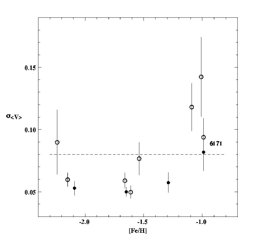
Figure 4: For a sample of globular clusters, the standard deviations of the $\langle V\rangle$ magnitudes of their RRLS are plotted as a function of the [Fe/H] values of the clusters. The open symbols are the values computed from the photographic photometry compiled by Sandage (1990). The solid symbols are the values computed from the CCD photometry (see text). Note the agreement between the photographic and the CCD values for NGC 6171. The dashed horizontal line is the value of $\sigma_{\langle V\rangle}$ that was adopted for the dispersion in $\Delta M_{V}^{\rm ev}$.

The star to star variation in $\langle V\rangle$ among the RRLS in a globular cluster, $\sigma_{\langle V\rangle}$, provides a measure of the dispersion in $\Delta M_{V}^{\rm ev}$ at fixed [Fe/H] because there is very little variation in [Fe/H] among the stars in a typical globular cluster. It is essential to calculate $\sigma_{\langle V\rangle}$ for a number of clusters that span a range in [Fe/H] because of the changes in track morphology makes $\sigma_{\langle V\rangle}$ larger for the metal rich clusters (see Sandage, 1990). Figure 4 shows the dependence of $\sigma_{\langle V\rangle}$ on [Fe/H], where we have plotted the values of $\sigma_{\langle V\rangle}$ that we calculated for the clusters M3, M15, M92, NGC 3201, 6171, 6712, 6723 and 6981 from the photographic photometry compiled by Sandage (1990). We ignored Sandage’s data for $\omega$Cen because its RRLS vary in [Fe/H] and for M4 because it has variable interstellar extinction across its face (Liu & Janes, 1990; Ivans et al., 2000, and references therein), which significantly increases the value of $\sigma_{\langle V\rangle}$. Accurate background subtraction is notoriously difficult in the crowded fields of globular clusters. Since it is done differently by the techniques of photographic and CCD photometry, we measured a few values of $\sigma_{\langle V\rangle}$ for clusters that had been observed by CCD cameras. The CCD photometry of the RRLS in NGC 6171 by Clement & Shelton (1997) yields a value of $\sigma_{\langle V\rangle}$ that agrees to within the errors with the photographic value, and the values that we obtained from the CCD photometry of M5 (Brocato et al., 1996), IC 4499 (Walker & Nemec, 1996), and M68 (Walker, 1994) are consistent with the measurements from the photographic photometry of other clusters that have similar metallicities. In all cases, the variation in $\langle V\rangle$ among the RRLS in a cluster is approximately Gaussian. Because very few halo RRLS are as metal rich as [Fe/H]$\sim-1$ (Suntzeff et al., 1991), we adopt $\sigma_{\langle V\rangle}=0.08$ for the dispersion in $\Delta M_{V}^{\rm ev}$. Figure 4 shows that this value is clearly an overestimate for all but the most metal rich RRLS.

While it is well known that the $M_{V}^{\langle{\rm HB}\rangle}$ varies with [Fe/H], there is much debate among different authors over the functional form of this variation and the values of $M_{V}$ at particular values of [Fe/H]. This has been reviewed by Cacciari & Clementini (2003), who obtained from a weighted average of ten methods in the literature the value of $0.59\pm 0.03$ for $M_{V}^{\langle{\rm HB}\rangle}$ at [Fe/H]$=-1.5$. While there is considerable evidence that $M_{V}^{\langle{\rm HB}\rangle}$ is a nonlinear function of [Fe/H], over the [Fe/H] range of halo RRLS ($-2.3\lesssim{\rm[Fe/H]}\lesssim-1$), most of the recently proposed $M_{V}^{\langle{\rm HB}\rangle}-$ [Fe/H] relationships can be closely approximated by a linear dependence with a slope of $0.23\pm 0.04$ (Chaboyer, 1999; Cacciari, 2003). We have therefore adopted the relationship:

$$M_{V}^{\langle{\rm HB}\rangle}=(0.23\pm 0.04)\,({\rm[Fe/H]}+1.5)+(0.59\pm 0.03)$$ (2)

Using the above $M_{V}^{\langle{\rm HB}\rangle}-$ [Fe/H] relationship, we can investigate the distance errors introduced by the adoption of one value of $M_{V}$ for all RRLS. An estimate of the likely distribution of [Fe/H] among the QUEST RRLS is provided the spectroscopic observations by Suntzeff et al. (1991) of 113 halo RRLS lying at galactocentric distances greater than 8.5 kpc. The distribution of these measurements is approximately Gaussian and has a mean value of [Fe/H]$=-1.65$ and a standard deviation, corrected for measuring errors, of 0.30 dex. These values are on the Zinn & West (1984) metallicity scale for globular clusters, which despite its age agrees well with recent determinations based on high dispersion spectroscopy (Kraft & Ivans, 2003). This metallicity dispersion and the uncertainties in the $M_{V}^{\langle{\rm HB}\rangle}$ relation produce $\sigma_{M_{V}^{\langle{\rm HB}\rangle}}=0.10$. When combined with our estimate of 0.08 for the dispersion in $\Delta M_{V}^{\rm ev}$, we obtain $\sigma_{M_{V}}=0.13$. Using the above estimates of the errors in the mean magnitudes and interstellar extinctions, we obtain 0.15 for the $1\sigma$ uncertainty in the true distance modulus for a typical RRLS in the QUEST survey. This translates into a fractional error ($\sigma_{r_{\sun}}/\!r_{\sun}$) of only 0.07. The distances to most other halo tracers have larger fractional errors, which for K giants (Dohm-Palmer et al., 2001) M giants (Majewski et al., 2003), and main-sequence stars (Juric et al., 2005; Newberg et al., 2002) are larger by factors of $\sim 2-3$. Only blue horizontal branch (BHB) stars, with fractional error estimates from $6-10\%$ (Brown et al., 2005; Sirko et al., 2004), are similar to the RRLS in the precision of their distance estimates. But BHB stars must be observed spectroscopically before they can be reliably separated from other types of blue stars. For determining the distances of the QUEST RRLS, we have adopted, as we have previously (e.g. Vivas et al., 2001), $M_{V}=0.55$, which is consistent to 0.01 mag. with the above $M_{V}-$[Fe/H] relation and the mean halo metallicity measured by Suntzeff et al. (1991).

Figure 5 shows a polar plot of the right ascension and extinction corrected mean magnitudes $V_{0}$, of the RRLS in the survey. The dotted circles indicate the values of $V_{0}$ corresponding to $r_{\sun}=$8, 19 and 49 kpc. This simple plot shows that the distribution of RRLS far from the Sun is not uniform. Particularly notable is the group of stars at $V_{0}\sim 19$, $\alpha=13\fh 0-15\fh 4$, which was reported earlier in Vivas et al. (2001). This feature, which is undoubtedly tidal debris from the Sgr dSph galaxy, is described in more detail later along with other density enhancements.

The positions of the RRLS in a Galactic Cartesian system have been calculated from their galactic coordinates, $l$ and $b$, and their heliocentric distances of the RRLS using the equations:

$$x = R_{0}-r_{\sun}\,\cos b\,\cos l$$

$$y = r_{\sun}\,\cos b\,\sin l$$ (3)

$$z = r_{\sun}\,\sin b$$

In this coordinate system, the $xy$-plane coincides with the galactic plane, with the line from the Galactic Center (GC) to the Sun defining the the $x$-axis. Positive $x$ values are on the Sun’s side of the GC and, the positive $y$ axis is in the direction of $l=90\arcdeg$. Coordinate $z$ is positive towards the North Galactic Pole. A value of 8 kpc was adopted for $R_{0}$, the distance of the Sun from the GC (Reid, 1993). Galactocentric distances are given by

$$R_{gal}=\sqrt{x^{2}+y^{2}+z^{2}}$$ (4)

Table 2 contains the galactic coordinates ($l$, $b$), extinction corrected V magnitude ($V_{0}$), galactocentric coordinates ($x$, $y$, $z$) and heliocentric and galactocentric distances, $r_{\sun}$ and $R_{gal}$. The ID numbers of the stars are the same as in Table 2 of Paper I. The full version of Table 2 is available only on-line as a machine-readable table.

5 THE SPACE DENSITIES

Although Figure 5 and several other recent halo surveys (see §1) have shown that the halo does not have smooth density contours, it is still useful to use this approximation to estimate the “background” of halo RRLS upon which density enhancements, such as the one described above, are overlaid. In this spirit, we have performed the following analysis.

Any determination of the space density of RRLS requires a careful consideration of the survey’s completeness. In Paper I we showed that the completeness of the RRc variables is significantly lower than that of the RRab , especially at the faint end of the survey. The sample of RRc may have also a small, but unknown, contamination from eclipsing binaries and variable blue stragglers (see Paper I). For these reasons, we have used only the RRab to estimate the density distribution. As we explained above, we do not use stars in the region with $\alpha=5-6$ hrs because of the large interstellar extinction. Finally, since the saturation limit of the different CCDs in the QUEST camera is not uniform (see Paper I), we eliminated stars with $\langle V\rangle<15.0$. This ensures that all distances are observed through the same solid angle. The space density of RRLS is calculated using a list of 334 RRab stars spread over $\sim 330$ deg² of the sky.

We followed Saha (1985) for calculating the number density of RRLS as a function of galactocentric distance $R_{gal}$. In this method, the total number of objects $N$ found in a solid angle $\omega$ is

$$N=\int{\omega\rho(r_{\sun})\,r_{\sun}^{2}\,dr_{\sun}}$$ (5)

Solving for the space density of RRLS, $\rho(r_{\sun})$,

$$\rho(r_{\sun})=\frac{1}{\omega r_{\sun}^{2}}\,\frac{dN}{dr_{\sun}}$$ (6)

The quantity $dN\!/dr_{\sun}$ is estimated from a plot of the cumulative number of RRLS versus $r_{\sun}$. First, all stars are sorted by increasing $r_{\sun}$. Then, for each star $i$ at a distance $r_{\sun i}$, $\,dN\!/dr_{\sun}$ is the local slope of the curve, which is calculated by fitting a straight line to the 3 contiguous points centered at $r_{\sun i}$. Finally, distances $r_{\sun}$ are transformed to galactocentric distances $R_{gal}$ using equation ( 4). This way, it is possible to calculate a space density at the $R_{gal}$ of each star (except for the ones at the extreme $r_{\sun}$’s).

As noted by Wetterer & McGraw (1996) this method works well for small solid angles, where a heliocentric distance corresponds to a unique galactocentric distance. Our survey has a big solid angle which covers a large range in galactic latitude and longitude, and Saha’s method will not work for such a region. Wetterer & McGraw proposed a variation of this method which was applied to their driftscan survey, similar in shape to ours, to calculate space densities based on a model of a spherical halo or a ellipsoidal one. We are interested here in studying the density profile of the halo along different lines of sight in order to see differences as a function of location in the Galaxy. Consequently, we divided our survey into small sub-regions, where it was possible to use Saha’s procedure. The size of the sub-regions must be large enough to contain a sufficient number of stars for the calculations, but small enough to cover only a small range in galactic coordinates. We divided our $2\fdg 3$-wide strip in 19 pieces of equal area. Each piece is 0.5 hr long in right ascension for an area of 16.5 deg² (the area covered by the gaps between CCDs has been subtracted). The number of RRab in each of these slices of sky varies from 5 to 33.

Figure 6 shows the line of sights of each of our sub-regions on the sky. The length of the arrows indicate the range in distance from the Sun covered in each sub-region which was calculated from the limits in V magnitude of the survey and the extinction in that particular direction. Table 3 has the coordinates and range of $R_{gal}$ covered in each sub-region. For comparison Figure 6 also shows, at the same scale, the lines of sight and depths of previous surveys of RRLS aimed to calculate the space density of the halo: the Lick survey (Kinman et al., 1965, 1966, 1982), the Palomar-Groningen survey (Plaut, 1966, 1968, 1971), Saha’s survey (Saha, 1985) and Hawkins’ survey (Hawkins, 1984). The area covered by each line of sight in those surveys (all photographic) varies from 16 to 43.6 deg² and each one has different degrees of completeness. The details of each survey are summarized in Wetterer & McGraw (1996) (see also Table 4-2 in Smith 1995). One of the Lick’s fields, MWF 361 or RR I, which has been extensively studied (Kinman et al., 1965, 1985; Preston et al., 1991), has partial overlap with our sub-region $\alpha=16\fh 0-16\fh 5$.

Because of its special shape and characteristics, Figure 6 does not include the CTI survey of Wetterer et al. (1996). The survey is similar to ours in the sense that it is a driftscan survey. It covers a very narrow strip ($8.\!^{\prime}3$) over all right ascensions for a total area of 36 deg², up to a distance $r_{\sun}$ of 30 kpc. Also, we do not show the RR Lyrae candidate searchs made with data from the SDSS (Ivezić et al., 2000, 2005) because their completeness are relatively low. The line of sights searched by Ivezić et al. (2000) have similar direction than ours (but longer) in the range of $\alpha=10\fh 7-15\fh 8$.

Figure 6 shows that our survey covers a wide area of the outer parts of the halo where few RRLS have been discovered. Of the previous surveys that identified RRLS by light curve and period, only Saha’s and Hawkins’ surveys ventured before in the $r_{\sun}>30$ kpc region of the halo. Notice that previous surveys were mostly made toward 3 directions: the galactic center, the galactic anti-center and the north galactic pole. Our survey provides a homogeneous sample of RRLS in a wide range of galactic coordinates.

In order to correct for incompleteness, the space density given by equation 6 was divided by the completeness of the survey in that part of the sky. The completeness for the RRab in the QUEST survey is high ($>80\%$) over most of the region but decreases toward the ends of the strip. The completeness was calculated using extensive simulations as a function of $\alpha$, separately for bright ($V<18.5$) and faint stars, and it is shown in Figure 10 of Paper I. Small corrections have been made to these completeness estimates because we removed the nonvariables mentioned in secton 2

The number density of RRLS as a function of $R_{gal}$ along the different lines of sight is shown in Figure 7. We have plotted also the space densities of RRLS in Lick field “RR I”, as determined by Preston et al. (1991), in the panel of $\alpha=16\fh 0-16\fh 5$. The fact that we get similar results in the range of distances of overlap give us confidence that our completeness estimates are correct. Preston et al. (1991) used a different method to estimate densities, which basically consists of calculating the volume occupied by a fixed number of stars of continuously increasing $r_{\sun}$.

The most striking feature of the density profiles of Figure 7 is the big over-density of RRLS at $R_{gal}>40$ kpc in the regions $\alpha=13\fh 0-15\fh 5$, which is due to the Sgr tidal tail (see also Figure 5).

6 SMOOTH DENSITY CONTOURS

Traditionally, the halo has been pictured as a region where the density contours smoothly vary with $R_{gal}$ as a power law:

$$\rho(R_{gal})=\rho_{0}(R_{gal}/\!R_{0})^{n}$$ (7)

where $\rho_{0}$ is the local space density of RRLS. The exponent $n$ has been determined by Wetterer & McGraw (1996) by combining the results of several surveys of RRLS and has a value of $n=-3.02\pm 0.08$. They fitted the power law using data with $R_{gal}$ from 0.6 to 80 kpc, with the caveat that only 9 objects with $R_{gal}>30$ kpc were available. Amrose & McKay (2001) have determined a value of $\rho_{0}=4.6\pm 0.4$ kpc^-3 with RRab stars from the first results of the ROTSE all-sky survey.

The power law with the above values is shown in the density profiles of Figure 7 as a reference. In principle, we do not expect a perfect fit of the data to a power law not only because of statistical fluctuations but also because the outer halo may be filled with sub-structures, as predicted by hierarchical models of galaxy formation (eg. Bullock et al. 2001). In fact there are several large regions of unexpectly high density in our survey, which are seen in Figure 7 as large departures from the solid lines at certain distances $R_{gal}$. Ignoring these over-densities, our first model, a spherical halo with a power-law density fall-off, does a fair job describing the density profiles along the different lines of sight, except in the regions with $\alpha>14$ h for which it over-estimates the space density of RRLS. As seen in Figure 6 and Table 3 these sub-regions have lines of sights approaching the galactic center and thus, they contain several objects at small $R_{gal}$. Since this power law reproduces well the space densities at larger $R_{gal}$, there is either a problem with the parameters of the power law or the assumption of an spherical halo.

Results from previous surveys toward the galactic center direction led several groups to propose density contours that are flatter in the inner halo (Kinman et al., 1965; Wesselink, 1987; Hawkins, 1984; Kinman et al., 1994). Preston et al. (1991) constructed an empirical model of a halo with variable flattening which fit simultaneously RRLS density profiles toward the north galactic pole and the GC. The model consists of isodensity contours described by ellipsoids of revolution of semi-major axis $a$, whose flattening $(c/\!a)$ is given by

$$c/\!a=\left\{\begin{array}[]{ll}(c/\!a)_{0}+[1-(c/\!a)_{0}](a/\!a_{u})&\mbox{if $a<a_{u}$}\\ 1&\mbox{if $a>a_{u}$}\end{array}\right.$$ (8)

with $(c/\!a)_{0}=0.5$ and $a_{u}=20$ kpc. Consequently, at large distances from the GC, this model has spherical density contours.

Our sample of RRLS provides a test of models with different halo shapes and whether they can simultaneously fit the data along all lines of sight. We tested 3 different models of the halo: a spherical one (shown in Figure 7), a flattened halo with constant $(c/\!a)=0.6$, and Preston et al. (1991)’s model with variable flattening.

In the non-spherical models, the density contours are described by

$$\rho(a)=\rho_{0}(a/\!R_{0})^{n}$$ (9)

where

$$a=\sqrt{x^{2}+y^{2}+\left(\frac{z}{(c/\!a)}\right)^{2}},$$ (10)

To see which model best describes our data, we calculated the standard deviation of the data points about the power law in each sub-region. For these calculations we left out the the most obvious over-densities of RRLS in Figure 7. Specifically, we did not include any star with $R_{gal}>40$ kpc in the range $13\fh 0<\alpha<15\fh 4$, because they are known to belong to the Sgr stream. We also took out some other stars causing notable over-densities: 3 stars at $R_{gal}\sim 18$ and $4\fh 5<\alpha<5\fh 0$; 5 stars at $R_{gal}\sim 20$ and $12\fh 0<\alpha<13\fh 0$; and the 5 known variables of the globular cluster Pal 5 at $R_{gal}\sim 17$ and $15\fh 0<\alpha<15\fh 5$. Except for the Sgr and Pal 5 stars, the elimination of the other over-densities made no significant differences in the results we describe here. With the parameters $\rho_{0}=4.6$ kpc^-3 and $\,n=-3.0$ the three models produce the dispersions that are plotted as functions of right ascension in Figure 8. As expected from Figure 7, the spherical halo (filled circles) produces large deviations at $\alpha>14$h. On the other hand, a halo with large, constant flattening (open triangles) yields a good fit of the data in the regions toward the GC ($\alpha>15\fh 5$), but it does not reproduce the observed density profile at high galactic latitudes ($9\fh 5<\alpha<14\fh 0$, see Figure 9a). In those regions, the power-law tends to underestimate the observed density of RRLS. The model with varying flattening yields the best fit since it produces small and similar standard deviations over all lines of sight (see Figure 10). In particular, this model provides a better description of the data than the spherical model at $\alpha>14h$ (cf. Figures 7 and 10).

The values of $n$ and $\rho_{0}$ used so far were both determined by assuming a spherical halo, and they may not be optimal for the other models. For example, Wetterer & McGraw (1996) found a steeper power law ($n=-3.53\pm 0.08$) when the variable flattening model was applied to their data. Also, a slightly higher value of the local density ($\rho_{0}=5.8\pm 0.7$ kpc^-3) is found by counting RRLS very close to the Sun, instead of averaging the value of the density at $R_{gal}=R_{0}$ in several directions of the Galaxy (Amrose & McKay, 2001). Therefore, we repeated the experiment with these other plausible density power laws and the best result was always found with the variable flattening model. For example, a steeper power law ($n=-3.5$) does not describe well the region of $\alpha=10\fh 5-11\fh 0$ with any model (Figure 9b) unless the local density takes a much higher value, which is then unreasonable for all other lines of sight and inconsistent with published measurements of that quantity.

We used the data over all the regions to derive the best parameters for a power law with all the tested models. The densities along all lines of sight were averaged in bins of equal size in $\log a$ (or $\log R_{gal}$ in the case of the spherical model) and fit by the method of least squares. The results are presented in Table 4. On average, both the flattened halo model and the variable flattening one produced the best overall fit to our data (lowest rms). However, we favored the variable flattening model because it best reproduces both the local density found by Amrose & McKay (2001), and the slope $n$ from previous works, including other tracers ($-3.5$ for Globular Clusters (Zinn, 1985) and BHB (Preston et al., 1991)). Notice that 52 stars with $R_{gal}>30$ kpc were used in the fit, $\sim$6 times more than the number used in previous studies (Wetterer & McGraw, 1996).

In Figure 11, the densities averaged over all lines of sight are compared with the best fitting profile of the variable flattening model. The fit is reasonable, but with a larger than expected number of points deviating by more than one standard deviation. This may be due to the failure of the model to account for the lumpy nature of the halo and the variations in the specific frequency of RRLS. Nonetheless, this model serves our purpose of providing a description of the ”background” of RRLS.

There is no evidence for a steeper power law ($n\sim-5$) beyond 25 kpc as was suggested by Saha (1985). The underdensity that he observed in one of his fields may be simply due to the clumpy nature of the outer halo. This might also be the explanation for the observation by Ivezic et al (2000) of an edge to the halo at 50-60 kpc (see Ivezic et al. 2004).

7 IDENTIFICATION OF OVERDENSITIES

We have performed the following analysis to identify overly dense regions that may escape detection by visually examining Figure 5. Many of these feature need to be confirmed by radial velocity and/or proper motion measurements. We have restricted this analysis to stars with $\langle V_{0}\rangle>14.8$ because at brighter magnitudes the differences in the saturation of limits of the CCDs in the QUEST camera produce some variation in completeness.

The first step in our analysis was the development of a computer code to recognize groups of RRLs that may be statistically significant. For each star ($i$) in the QUEST catalogue, the code computed the distances ($d_{ij}$) from $i$ to each of the other stars $j$ and kept as neighbors the stars within a distance limit ($d_{limit}$). It then created a ranking of the $d_{ij}$ values of the neighbors and computed the volumes centered on star $i$ that included in turn each of its more distant neighbors. Because the QUEST survey is limited in $\delta$ to $2.3\arcdeg$, these volumes are non-spherical, and we approximated them with cylinders with heights in the $\delta$ direction. Each volume contains star $i$, the star $j$ at distance $d_{ij}$ and all stars with smaller distances from star $i$, if any. The number of stars observed in a volume, $n_{obs}$, was then compared with the number expected in the absence of an overdensity. Our model for the density contours (see above) provides the number density of RRab variables at the position of star $i$. These densities were then multiplied by factors that take into account the incompleteness of survey in type ab and in type c variables, which vary with $\alpha$ and $\langle V\rangle$ (Paper I). The resulting number density for all types of RRLS was then multiplied by the volume to yield $n_{exp}$ , the expected number of RRLS, which was rounded to the nearest integer. We then computed the probability, $P$, that $N\geq n_{obs}$, given that $N$ is a random number following a Poisson distribution of mean $n_{exp}$,

$$P(n_{obs},\infty,n_{exp})=1-\sum_{x=0}^{x=n_{obs}-1}P(x,n_{exp})$$ (11)

Star $i$ and each of its neighbors that occupy a volume where $P\leq P_{limit}$ are considered members of a group. If none of these stars has been previously assigned to a group, then a new group number is assigned. Otherwise, they are considered additional members of the previously assigned group. In addition to group number, star $i$ is tagged by the lowest $P\leq P_{limit}$ that occurred in the calculations of the values of $P$ for the small volumes.

The free parameters in this analysis are the choices for $d_{limit}$ and $P_{limit}$. For $d_{limit}$, we chose $0.18\,r_{\sun}$, which is approximately $2.5\,\sigma_{r_{\sun}}$. Consequently, two stars that lie at the same distance and direction have a probability of $\sim 0.99$ of being considered neighbors in this analysis. Increasing $d_{limit}$ significantly above this value produces overlap between what may be separate over-densities. Decreasing $d_{limit}$ significantly may mean that some small over-densities are missed because of distance errors. For $P_{limit}$, we chose the value $1.0\times 10^{-3}$, which at first glance may appear smaller than necessary. Because there are 457 stars in the revised QUEST catalogue and a minimum of a few stars within $d_{limit}$ of each, thousands of calculations of $P$ are made. It is fairly common for random fluctuations alone to produce a few small groups with $P\leq 1\times 10^{-3}$, as our Monte Carlo simulations indicate (see below).

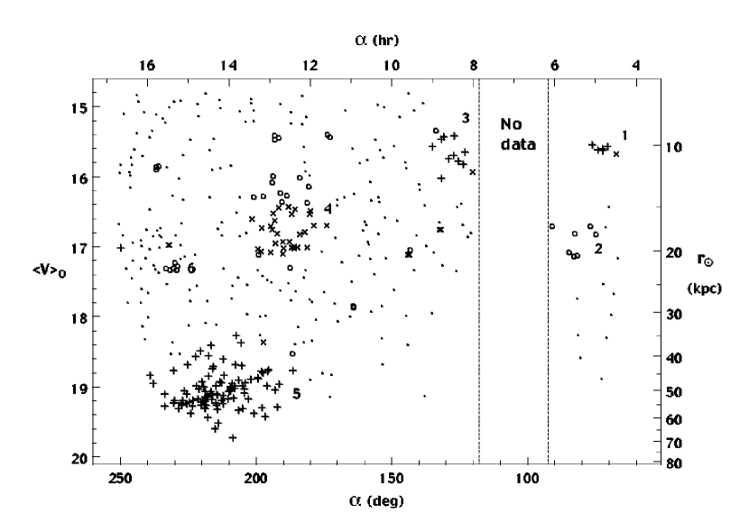
Figure 12: The values of mean V magnitude, corrected for extinction, of the QUEST RRLS are plotted against right ascension. The 5 RRLS in the globular cluster Pal 5 have been removed from this sample. The crosses, $\times$’s, and open circles depict the RRLS that are assigned to groups with high, medium, and low confidence, respectively. The small dots are RRLS that do not belong to groups according to our group finding routine. The six most significant groups are numbered in order of increasing $\alpha$.

In Figure 12, we have used different symbols to indicate the confidence that we attach to a star’s membership in an overdensity. Values of $P$ in the ranges $1\times 10^{-3}\geq P>1\times 10^{-4}$ , $1\times 10^{-4}\geq P>1\times 10^{-5}$ , and $P\leq 1\times 10^{-5}$ indicate with low, medium, and high confidence, respectively, that a star is considered part of an overdensity. We must emphasize that some of the stars identified as belonging to a group will turn out to be clearly nonmembers once their motions are measured because every overdensity is overlaid on a ”background” of unrelated RRLS. We are therefore identifying stars that are candidate members of the groups, and their $P$ values provide an estimate of relative likelihood of membership. The sparse globular cluster Pal 5 lies within the survey region (see Figure 5). Not surprisingly, its five RRLs, which were all detected by the QUEST survey, produce a very significant overdensity which is not of interest because the cluster has been known for decades. We therefore removed these 5 stars from the survey before performing the search for overdensities. One of the identified overdensities is in close proximity to Pal 5 and is undoubtedly related (see below). For each overdensity recognized by the above procedure, the quantity $P_{ave}$ was calculated by averaging the $P$ values that were assigned each member of the group. The above limits on $P$ have also been applied to $P_{ave}$ in order to identify groups of low, medium, and high confidence. The groups that seem most likely to be real and their confidence category are listed in Table 5, where also are listed the position of the group in Figure 12, the number of members ($n_{obs}$), $P_{ave}$, and the frequency ($F$) with which a similar group occurred by chance in the Monte Carlo calculations. $F$ is equal to the total number of groups with $N\geq n_{obs}$ and average $P\leq P_{ave}$ that were produced by the simulated surveys divided by the total number of artificial surveys ($1\times 10^{4}$).

In the Monte Carlo simulations, the volume of the galactic halo covered by the QUEST survey was subdivided by $\alpha$ into intervals of 0.25 hours ($3\fdg 75$) and by $\langle V_{0}\rangle$ into intervals of 0.25 mag. No subdivision was made by $\delta$. The position in the Galaxy of the center of each subdivision was computed using $M_{V}=+0.55$ for RRLS, and the number density of RRab at this position was calculated from our model for the background of type ab RRLS. This number density was corrected for the incompleteness of the QUEST survey using the same factors that were used with the real survey. It was then multiplied by the volume delineated by the intervals in $\alpha$, $\delta$, and $\langle V_{0}\rangle$. After rounding to the nearest integer, this yielded $n_{exp}$ for the volume. To provide for statistical variation, we computed a random number ($N$) from a Poisson distribution (a Poisson deviate) with mean equal to $n_{exp}$, which employed a random number as a seed variable. These $N$ artificial stars were then randomly distributed in $\alpha$, $\delta$, and $\langle V_{0}\rangle$ within the limits of the subdivision using random a number generator with different seed values for each quantity. The calculation then proceeded to the next subdivision where $n_{exp}$ was again calculated for the new position and different random selections were made for the seed variables in the calculation of the Poisson deviate and in the distribution of the stars in position and in magnitude. These calculations were continued until the area of the QUEST survey was covered. The program for identifying overdensities that we described above was then used to find and characterize any groups that were produced in this artificial survey.

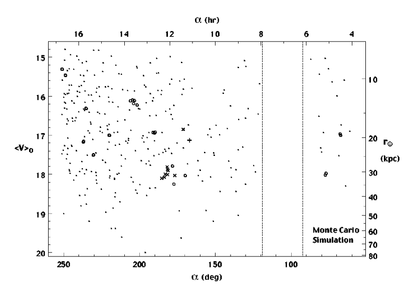
Figure 13: For a typical Monte Carlo simulation of the QUEST RRLS survey, mean V magnitude, corrected for extinction, is plotted against right ascension. The artificial stars depicted as crosses, $\times$’s, and open circles are assigned to groups with high, medium, and low confidence, respectively. The small dots are artificial stars that are not assigned to groups. The large group at $\alpha\sim 180$ and ${langleV\rangle}_{0}\sim 18$ and all other clusterings in this diagram are due to statistical fluctuations.

In order to see what size groups and their $P_{ave}$ values that might have arisen by chance in the QUEST survey, a total of $1\times 10^{4}$ artificial surveys were produced by starting each Monte Carlo calculation with a different seed value. Each of these surveys was fed to the program for finding overdensities and the values of the frequencies $F$ (see above) were computed. Experiments with different sizes for the intervals in $\alpha$ and $\langle V_{0}\rangle$ showed that these Monte Carlo calculations were not particularly sensitive to their choices as long as the intervals were not so large to encompass a significant variation in number density and not so small that $n_{exp}=0$ for many subdivisions. One of these artificial surveys, which is typical in terms of the number and sizes of overdensities, is displayed in Figure 13. The artificial stars that are in overdensities are labeled in exactly the same manner as the stars in RRLS in the real survey. Since the same model for the smoothed density contours was used both to generate the artificial survey and to identify the overdensities, the ones that appear in the artificial surveys are entirely due to statistical fluctuations. Once can see from this figure that random variations alone can produce significant overdensities, even ones that meet our criteria for the high confidence category. Not surprisingly, the majority of the randomly occurring overdensities contain very few stars.

8 DISCUSSION

Table 5 lists the 6 most significant overdensities in the QUEST survey according to our group finding routine. With the exception of Group 2, we will discuss each of these groups in order of their sizes. Group 2 lies in the region of the survey where the interstellar extinction is high and variable. Because our estimate of the completeness of the survey in this region is suspect, we consider Group 2 to be only a marginal detection of halo substructure.

8.1 Group 5, The Sagittarius Stream

The largest and by far the most significant over-density is Group 5, at a mean distance of 50 kpc, which was produced by the tidal destruction of the Sgr dSph galaxy. According to our group finding routine, Group 5 contains 104 candidate members, which is $23\%$ of the whole sample of QUEST RRLS. Its $F$ value (see Table 5) indicates that none of the $10^{4}$ Monte Carlo simulations produced a group of this size or larger with $P<P_{ave}$ .

This striking overdensity was discovered in the spatial distribution of A stars (Yanny et al., 2000) and RRLS candidates (Ivezić et al., 2000). Shortly thereafter, a main-sequence was found in the color-magnitude diagram of a small region (Martínez-Delgado et al., 2001). It has also been detected in the distributions of carbon stars (Ibata et al., 2001), F type main-sequence stars (Newberg et al., 2002), and M giants (Majewski et al., 2003). Our initial results from the QUEST survey (Vivas et al., 2001) provided additional evidence for a large overdensity of RRLS. The distributions of these stars and the measurements of radial velocities for subsamples (e.g. Dohm-Palmer et al., 2001; Majewski et al., 2004; Vivas et al., 2005) provide conclusive proof that this feature is part of the leading stream from the Sgr dSph galaxy. Figures 5 and 12 show that there are very few QUEST RRLS at large $r_{\sun}$ that are not part of Group 5. This observation and similar ones using the different types of stars mentioned above illustrate that the debris from the Sgr dSph galaxy is a major contributor to the outer galactic halo.

8.2 Group 4, the “12.4 h clump”, the “Virgo Stellar Stream” and the “Virgo Overdensity”

Group 4, which after the Sgr Stream is the most prominent feature in Figures 5 and 12, contains 42 potential members. The $F$ value of this group (Table 5) indicates that a few of the Monte Carlo simulations produced artificial groups of equal or larger size and significance. Based on this information alone, there is a small, but not negligible probability, that this feature is an artifact.

The eastern edge of this feature was identified as an overdensity in our first report of QUEST results (Vivas et al., 2001). It became known as the “12.4 h clump” when its large size was recognized in the completed QUEST survey (Vivas, 2002; Vivas & Zinn, 2003). The survey of F type main-sequence stars in the SDSS (Newberg et al., 2002) also revealed its large size. Figure 12 shows that it spans $12\leq r_{\sun}\leq 20$ and $175\leq\alpha\leq 205$ , which corresponds to a span of $\sim 9$ kpc at the mean of 17 kpc.

The densest part of this feature is located at $\alpha\sim 186\arcdeg$ and $r_{\sun}\sim 17$ kpc. Very recently, Duffau et al. (2006) have shown that a subsample of the QUEST RRLS in this dense region and a subsample of the BHB stars in the same region of space from the Sirko et al. (2004) survey have very similar radial velocities, indicating that they are part of a stellar stream. The RRLS in the stellar stream have a low mean metallicity but a wide range in metallicity, which suggests that they are the debris from a low luminosity dSph galaxy. Duffau et al. (2006) have suggested the name the Virgo Stellar Stream (VSS) for this feature of halo substructure, which they have traced over 106 deg² of the sky. Until more radial velocity measurements are obtained, it is not clear that majority the stars of Group 4 belong to the VSS. Duffau et al. (2006) noted that in addition to the VSS there is less significant evidence for two other moving groups containing smaller numbers of RRLS and BHB stars, which may be a sign of that there is more to Group 4 than the VSS.

Group 4 also lies in the direction of the “ Virgo Overdensity” that has been recently identified by Juric et al. (2005) in distribution of main-sequence stars in the latest photometry of the SDSS. They estimate that this feature covers $>1000$ deg² of the sky and lies in the range $5\leq r_{\sun}\leq 15$ kpc. It therefore overlaps considerably with Group 4, and considering distance errors of $\sim 20\%$ for the main-sequence stars, it also overlaps with the known members of the VSS, which lie at its distant edge. Juric et al. (2005) suggest that this feature is the tidal stream from a dwarf galaxy or possibly the galaxy itself. While the exact relationships between the VSS, the Virgo Overdensity, and Group 4 are unclear at this moment, there is no doubt that at least part of Group 4 is a real halo substructure.

8.3 Groups 1 and 3, the Monoceros Stream?

The next two most significant groups, Groups 1 and 3, may be related to each other. They lie at similar values of $r_{\sun}$ on either side of the region skipped by the QUEST survey because of the severe crowding of star images near the galactic plane. The low $F$ values of these groups suggest that they are likely to be real. Group 1 is the less certain of the two because it lies in the range of $\alpha$ where it was difficult to estimate the completeness of the survey. Spectroscopic observations have been obtained for many of the stars in these groups and will be discussed in a later paper.

As we noted in a preliminary report of our results (Zinn et al., 2004), Groups 1 and 3 lie approximately in the same direction and at the same distance as the Monoceros Stream that was discovered by Newberg et al. (2002) in the SDSS photometry and confirmed by the spectroscopic observations of Yanny et al. (2003). This stream appears to be part of large-ring like structure that envelops the Milky Way (see also Majewski et al., 2003; Ibata et al., 2003; Rocha-Pinto et al., 2003; Peñarrubia et al., 2005; Conn et al., 2005a, b). It is widely interpreted as the debris of tidally disrupted dwarf galaxy, but it is clearly not part of the Sgr Stream nor any of the other halo overdensities that we have discussed above. While the association of Groups 1 and 3 with the Mon Stream appears likely, this is not certain. The measurements by Kinman et al. (2004) of the radial velocities of a sample of RRLS in the anticenter direction did not reveal any that clearly belong to the Mon Stream.

8.4 Group 6, the overdensity near Pal 5

As we noted above, we purposely removed the 5 RRLS in the globular cluster Pal 5 from the QUEST catalogue before searching for overdensities. Group 6 lies very close to Pal 5 and at exactly the same distance, which of course suggests a relationship with the cluster. Consequently, we discount the relatively large $F$ value of Group 6, which suggests that the QUEST survey is expected to contain one or two groups of the size and significance of Group 6 that are nothing more than statistical fluctuations.

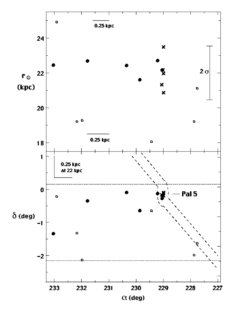
Figure 14: These diagrams show the RRLS in the vicinity of the globular cluster Pal 5. The $\times$’s are the five previously known RRLS in Pal 5. The QUEST values of $\langle V_{0}\rangle$ were used in the calculation of their distances. The solid circles are the RRLS belonging to Group 6. The small open circles are other QUEST RRLS. The dashed horizontal lines in the lower diagram show the declination limits of the QUEST survey. The other dashed lines delineate the boundaries of the tidal tails of Pal 5 (Odenkirchen et al., 2003).

In the top diagram of Figure 14, we have plotted the 5 previously identified RRLS in Pal 5, the 6 stars in Group 6, and other QUEST RRLS in the region. The bottom diagram of Figure 14 shows the distribution of the same stars on the sky along with a rough outline of Pal 5 and its tidal tails, as revealed by the analysis of SDSS photometry by Odenkirchen et al. (2001, 2003). One can see from the upper diagram that all 6 stars in Group 6 lie at the same $r_{\sun}$ as Pal 5 to within the errors. Two of the Group 6 stars, RRLS 403 and 405, lie approximately 9.2 and 11.2 arcmin., respectively, from the cluster center (see lower diagram). The extensive photometry of Odenkirchen et al. (2002) shows that there are many Pal 5 stars at similar angular distances; consequently the association of these RRLS with the cluster is nearly certain. Another RRLS (393), which was not identified as member of Group 6 because it lies too far away from the group’s center is also likely to have been once a member of Pal 5. Its position on the sky and distance are consistent with it being part of the southern tidal stream from Pal 5. It is interesting to note that Pal 5 has been considered odd among globular clusters because all five of its previous known RRLS are type c. Two of the three probable members identified here are type ab, which partially removes the imbalance in the numbers of these types of variables.

It is less certain that any of the other members of Group 6 are related to Pal 5, for they are offset from the cluster to the east by significant amounts. However, as reported in Zinn et al. (2004), our preliminary measurements suggest that the two members of Group 6 near $\alpha\sim 230\arcdeg$ have radial velocities and metallicities that are consistent with membership in the cluster. This possibility is being explored as the measurements are refined.

8.5 Other Overdensities

One can see from Figure 5 that the group finding routine has identified a number of other small groups. While the $F$ values of these groups suggest that they may be not be real, this cannot be discounted entirely until their motions are measured. Kinman et al. (2004) have shown that small groups of co-moving RRLS exist in the halo, which they suggest may be the remains of disrupted globular clusters. Our spectroscopy of few of the small groups in the QUEST survey will be reported later.

9 Summary

Our major result is that the Galactic halo contains substructures over a spectrum of sizes. While much remains to be learned about the features identified here and by other surveys, there is strong evidence that at least some were produced by the merger of smaller galaxies with the Milky Way. These merger events have clearly deposited a large number of stars in the halo, as predicted by models of the hierarchical picture of galaxy formation (e.g. Bullock & Johnston, 2005). While this may seem so obvious now, it represents a large departure from the traditional picture of the galactic halo that could be characterized by smooth density contours and a power-law drop-off.

Figure 3: Extinction in V magnitude of the RRLS in the QUEST survey plotted as a function of right ascension.

Figure 5: Radial plot of the distribution of the RR Lyrae stars in right ascension. The radial axis is the extinction corrected $\langle V\rangle$ magnitudes. All stars are located in a $2.3^{\circ}$ wide strip centered at declination $-1^{\circ}10^{\prime}.8$. The circles correspond to a distance from the Sun of 8, 19 and 49 kpc. The solid line indicates the position of the galactic plane, which is located approximately in the GC and Galactic anticenter direction ($l\sim 32\arcdeg$ and $l\sim 214\arcdeg$). The globular cluter Pal 5 is located at $\alpha\sim 229\arcdeg$ and $\langle V_{0}\rangle\sim 17.3$.

Figure 6: Left: Line of sights of each sub-region in the QUEST survey in galactic coordinates. The labels indicate right ascension. Right: Other surveys for RRLS in the halo: Lick (L), Palomar-Groningen (PG), Saha’s (S) and Hawkins (H)

Figure 7: Number of RRLS per unit volume as a function of galactocentric distance. Each panel represents a different line of sight which covers the right ascension range indicated in the lower left corners. The $\times$’s in the panel corresponding to $\alpha=16\fh 0-16\fh 5$ are the space densities calculated by Preston et al. (1991) for Lick’s field RR I, which partially overlaps that sub-region. The lines show a power law with $\rho_{0}=4.6$ kpc^-3 and $n=-3.0$.

Figure 8: Standard deviation of the data points to a density power law with $\rho_{0}=4.6$ kpc^-3 and $n=-3.0$ for the 3 different models discussed in the text: a spherical halo (solid circles), flattened halo with c/a=0.6 (open triangles) and variable flattening ($\times$’s).

Figure 9: Examples of models that do not fit the observed space density of RRLS (a) A flattened halo ($(c/\!a)=0.6$) underestimates the density $\rho$ at high galactic latitudes, for example in the panel corresponding to $\alpha=12\fh 0-12\fh 5$ ($b\sim 60^{\circ}$). (b) A steeper power law ($n=-3.5$) does not reproduce the density profile at $\alpha=10\fh 5-11\fh 0$, not even with the variable flattening model

Figure 10: Same as Figure 7 but for the model of variable flattening of the halo. Notice that the $x$-axis is now $a$, the semi-major axis of the ellipsoids, which is equal to $R_{gal}$ for $a\geq 20$ kpc.

Figure 11: Averaged space density profile of RRLS using the variable flattening model for the halo. The solid line is the best fitted power law with $n=-3.1$ and $\rho_{0}=4.2$ kpc^-3. Error bars are the standard deviations of the mean density in each bin.

Table 1: The Specific Frequencies of RR Lyrae Variables in Dwarf Spheroidal Galaxies

Galaxy	$M_{V}$	[Fe/H]	$N_{obs}$	$N_{est}$	$S_{RR}$
Carina	$-8.6\pm 0.5$	-2.0	75	76	$28\pm 6$
Draco	$-8.4\pm 0.2$	-2.0	268	268	$117\pm 12$
Fornax	$-13.0\pm 0.3$	-1.3	515	660	$4.2\pm 0.2$
Leo I	$-11.5\pm0.3$	-1.5	74	74	$1.9\pm0.2$
Leo II	$-9.6\pm 0.3$	-1.9	148	148	$21\pm2$
Sagittarius	$-13.9\pm 0.5$	-1.0	1700	5200	$14.3\pm 0.2$
Sculptor	$-10.7\pm 0.5$	-1.8	226	500	$26\pm1$
Sextans	$-9.2\pm 0.5$	-1.7	111	260	$54\pm 7$
Ursa Minor	$-8.4\pm 0.5$	-2.2	82	84	$37\pm9$
And I	$-11.8\pm 0.1$	-1.5	99	582	$11.1\pm 0.5$
And II	$-12.6\pm 0.2$	-1.5	72	400	$3.7\pm0.2$
And III	$-10.2\pm 0.3$	-1.9	51	204	$17.0\pm 1.3$
And VI	$-11.5\pm 0.2$	-1.6	111	529	$13.3\pm 0.6$

References. — Values of $N_{obs}$ taken from: Car: Dall’Ora et al. (2003); Dra: Kinemuchi et al. (2002); For: Bersier & Wood (2002); Leo I: Held et al. (2001); Leo II: Siegel & Majewski (2000); Sgr: Cseresnjes (2001); Scl: Kaluzny et al. (1995); Sex: Lee et al. (2003); UMi: Nemec et al. (1988); And I & And III: Pritzl et al. (2005); And II: Pritzl et al. (2004); And VI: Pritzl et al. (2002)

Table 2: Galactic coordinates and distances of the RRLS

ID	$l$ (∘)	$b$ (∘)	$V_{0}$	$x$ (kpc)	$y$ (kpc)	$z$ (kpc)	$r_{\sun}$ (kpc)	$R_{gal}$ (kpc)
217	299.05	61.87	16.23	4.9	-5.7	12.1	13.7	14.2
218	299.38	60.74	14.53	6.5	-2.7	5.4	6.2	8.9
219	299.42	61.98	14.79	6.4	-2.9	6.2	7.0	9.4
220	300.00	60.95	18.96	-3.7	-20.2	42.0	48.0	46.8
221	300.19	61.79	16.43	4.4	-6.1	13.2	15.0	15.3

Table 3: Coordinates of the sub-regions of the survey

$\alpha$ (h)	$l$ (∘)	$b$ (∘)	$R_{gal}$ (kpc)
4.5 - 5.0	198.2	-28.3	15 - 70
8.0 - 8.5	223.7	18.0	14 - 69
8.5 - 9.0	227.7	24.5	14 - 70
9.0 - 9.5	232.2	30.9	13 - 69
9.5 - 10.0	237.3	37.1	13 - 66
10.0 - 10.5	243.3	43.0	13 - 67
10.5 - 11.0	250.5	48.6	12 - 65
11.0 - 11.5	259.5	53.5	11 - 64
11.5 - 12.0	270.7	57.6	11 - 66
12.0 - 12.5	284.2	60.5	10 - 65
12.5 - 13.0	299.5	61.8	10 - 63
13.0 - 13.5	315.3	61.3	9 - 62
13.5 - 14.0	329.7	59.1	8 - 62
14.0 - 14.5	341.9	55.4	7 - 60
14.5 - 15.0	351.7	50.8	7 - 59
15.0 - 15.5	359.6	45.5	6 - 55
15.5 - 16.0	6.1	39.7	5 - 51
16.0 - 16.5	11.6	33.6	5 - 50
16.5 - 17.0	16.3	27.3	4 - 45

Table 4: Best parameters for models of the Halo

Model	$n$	$\rho_{0}$ (kpc-3)	rms
Spherical (c/a=1.0)	$-2.5\pm 0.1$	$2.0\pm 0.2$	0.14
Constant flattening (c/a=0.6)	$-2.7\pm 0.1$	$6.6^{+0.8}_{-0.7}$	0.11
Variable flattening	$-3.1\pm 0.1$	$4.2^{+0.5}_{-0.4}$	0.11

Table 5: The Most Significant Overdensities

Group	$n_{obs}$	$\alpha$	$\delta$	$l$	$b$	$\langle V_{0}\rangle$	$r_{\sun}$	$R_{gc}$	$P_{ave}$	Confidence	$F$	Comments
1	6	72	-1.0	199	-28	15.6	10.2	17.5	$4.6\times 10^{-6}$	high	0.0090	Mon Stream?
2	7	82	-0.9	204	-19	16.9	18.8	26.0	$7.9\times 10^{-4}$	low	1.1521
3	12	128	-1.3	226	22	15.7	10.5	16.8	$2.7\times 10^{-5}$	medium	0.0101	Mon Stream?
4	42	189	-0.8	296	62	16.7	17.0	17.2	$1.4\times 10^{-4}$	low	0.0032	Virgo feature
5	104	214	-1.1	342	55	19.0	50.2	46.5	$1.9\times 10^{-6}$	high	0.0000	Sgr Stream
6	6	230	-0.5	2	45	17.3	22.3	17.6	$7.3\times 10^{-4}$	low	1.3848	close to Pal 5

References

- Amrose & McKay (2001) Amrose, S. & McKay, T. 2001, ApJ, 560, L151
- Bersier & Wood (2002) Bersier, D. & Wood, P. R. 2002, AJ, 123, 840
- Brocato et al. (1996) Brocato, E., Castellani, V. & Ripepi, V. 1996, AJ, 111, 809
- Brown et al. (2005) Brown, W. R., Geller, M. J., Kenyon, S. J., Kurtz, M. J., Allende Prieto, C., Beers, T. C. & Wilhelm, R. 2005, AJ, 130, 1097
- Bullock et al. (2001) Bullock, J. S., Kravtsov, A. V. & Weinberg, D. H. 2001, ApJ, 548, 33
- Bullock & Johnston (2005) Bullock, J.S. & Johnston, K. V. 2005, ApJ, 635, 931
- Cacciari (2003) Cacciari, C. 2003, ASPC 296, 329
- Cacciari & Clementini (2003) Cacciari, C. & Clementini, G. 2003, Lect. Notes Phys., 635, 105
- Carraro & Lia (2000) Carraro, G. & Lia, C. 2000, å, 357, 957
- Carraro et al. (2005) Carraro, G., Vázquez, R. A., Moitinho, A. & Baume, G. 2005, ApJ, 630, L153
- Chaboyer (1999) Chaboyer, B. 1999, in Post-Hipparcos Cosmic Candles, Eds. A. Heck & F. Caputo, Kluwer Ac. Pub., 111
- Clement & Shelton (1997) Clement, C. M. & Shelton, I. 1997, AJ, 113, 1711
- Conn et al. (2005a) Conn, B. C., Lewis, G. F., Irwin, M. J., Ibata, R. A., Ferguson, A. M. N., Tanvir, N. & Irwin, J. M. 2005, MNRAS, 362, 475
- Conn et al. (2005b) Conn, B. C., Martin, N. F., Lewis, G. F., Ibata, R. A., Bellazzini, M. & Irwin, M. J. 2005, MNRAS, 364, L13
- Cseresnjes (2001) Cseresnjes, P. 2001, A&A, 375, 909
- Dall’Ora et al. (2003) Dall’Ora, M. et al. 2003, AJ, 126, 197
- Dohm-Palmer et al. (2001) Dohm-Palmer, R. C. et al. 2001, ApJ, 555, 37
- Duffau et al. (2006) Duffau, S., Zinn, R., Vivas, A. K., Carraro, G., Méndez, R. A., Winnick, R. & Gallart, C. 2006, ApJ, 636, L97
- Freeman & Bland-Hawthorn (2002) Freeman, K. & Bland-Hawthorn, J. 2002, ARA&A, 40, 487
- Gnedin & Ostriker (1997) Gnedin, O. Y. & Ostriker, J. P. 1997, ApJ, 474, 223
- Grillmair et al. (1995) Grillmair, C. G., Freeman, K.C., Irwin, M. & Quinn P.J. 1995, AJ, 109, 2553
- Harding et al. (2001) Harding, P., Morrison, H.L., Olszewski, E. W., Arabadjis, J., Mateo, M., Dohm-Palmer, R.C., Freeman, K.C. & Norris, J.E. 2001, A.J., 122, 1397
- Harris (1996) Harris, W.E. 1996, AJ, 112, 1487
- Hawkins (1984) Hawkins, M. R. S. 1984, MNRAS, 206, 433
- Held et al. (2001) Held, E. V., Clementini, G., Rizzi, L., Momany, Y., Saviane, I. & Di Fabrizio, L. 2001, ApJ, 562, L39
- Ibata et al. (2001) Ibata, R., Lewis, G., Irwin, M., Totten, E. & Quinn, T. 2001a, ApJ, 551, 294
- Ibata et al. (2003) Ibata R., Irwin, M., Lewis, G., Ferguson, A. & Tanvir, N. 2003, MNRAS, 340, L21
- Ideta & Makino (2004) Ideta, M. & Makino, J. 2004, ApJ, 616, L107
- Irwin & Hatzidimitriou (1995) Irwin, M. & Hatzidimitriou, D. 1995, MNRAS, 277, 1354
- Ivans et al. (2000) Ivans, I. I., Sneden, C., Kraft, R. P., Suntzeff, N. B., Smith, V. V., Langer, G. E., & Fulbright, J. P. 2001, RevMexAA (Serie de Conferencias) 10, 21
- Ivezić et al. (2000) Ivezić, Ž. et al. 2000, AJ, 120, 9631
- Ivezić et al. (2004) Ivezić, Ž. et al. 2004, in ASP Conf Ser. 327, Satellite and Tidal Streams, ed. F. Prada, D. Martinez-Delgado & T. Mahoney, 104
- Ivezić et al. (2005) Ivezić, Ž., Vivas, A. K., Lupton, R. & Zinn, R. H., 2005, AJ, 129, 1096
- Johnston et al. (1996) Johnston, K. V., Hernquist, L., & Bolte, M. 1996, ApJ, 465, 278
- Juric et al. (2005) Juric, M. 2005, astro-ph/0510520
- Kaluzny et al. (1995) Kaluzny, J., Kubiak, M., Szymanski, M., Udalski, A., Krzeminski, W. & Mateo, M. 1995, A&AS, 112, 407
- Kinemuchi et al. (2002) Kinemuchi, K., Smith, H. A., Lacluyzé, A. P., Clark, C. L., Harris, H. C., Silbermann, N. & Snyder, L. A. 2002, in Radial and Nonradial Pulsations as Probes of Stellar Physics, eds. C. Aerts, T. R. Bedding and J. Christensen-Dalsgaard, ASP Conf. Series, 259, 130
- King (1962) King, I. 1962, AJ, 67, 471
- Kinman et al. (1965) Kinman, T. D., Wirtanen, C. A. & Janes, K. A. 1965, ApJS, 11, 223
- Kinman et al. (1966) Kinman, T. D., Wirtanen, C. A. & Janes, K. A. 1965, ApJS, 13, 379
- Kinman et al. (1982) Kinman, T. D., Mahaffey, C. T. & Wirtanen, C. A. 1982, AJ, 87, 314
- Kinman et al. (1985) Kinman, T. D., Kraft, R. P., Friel, E. & Suntzeff, N. B. 1985, AJ, 90, 95
- Kinman et al. (1994) Kinman, T. D., Suntzeff, N. B. & Kraft, R. P. 1994, AJ, 108, 1722
- Kinman et al. (2004) Kinman, T. D., Saha, A. & Pier, J. R. 2004, ApJ, 605, L25
- Kraft & Ivans (2003) Kraft, R. P. & Ivans, I. I. 2003, PASP, 115, 143
- Kukarkin (1973) Kukarkin, B. V. 1973, in Variable Stars in Globular Clusters, IAU Colloquium 21, ed. J. D. Fernie, 8
- Layden (1998) Layden, A. C. 1998, AJ, 115, 193
- Lee et al. (2003) Lee, M. G. et al. 2003, AJ, 126, 2840
- Leon et al. (2000) Leon, S., Meylan, G. & Combes, F. 2000, A&A, 359, 907
- Liu & Janes (1990) Liu, T. & Janes, K. A. 1990, ApJ, 360, 561
- Majewski et al. (2003) Majewski, S. R., Skrutskie, M. F., Weinberg, M. D. & Ostheimer, J. C. 2003, ApJ, 599, 1082
- Majewski et al. (2004) Majewski, S. R. et al. 2004, AJ, 128, 245
- Martínez-Delgado et al. (2001) Martínez-Delgado, D., Aparicio, A., Gḿez-Flechoso, M. A. & Carrera, R. 2001, ApJ, 549, L199
- Martínez-Delgado et al. (2005) Martínez-Delgado, D., Butler, D. J., Rix, H-W., Franco, Y. I., Peñarrubia, J., Alfaro, E. J. & Dinescu, D. I. 2005, ApJ, 633, 205
- Martin et al. (2004) Martin, N. F., Ibata, R. A., Bellazzini, M., Irwin, M. J., Lewis, G. F. & Dehnen, W. 2004, MNRAS, 348, 12
- Mateo (1998) Mateo, M. 1998, ARA&A, 36, 435
- McConnachie & Irwin (2006) McConnachie, A. W. & Irwin, M. J. 2006, MNRAS, 365, 1263
- Momany et al. (2004) Momany, Y., Zaggia, S. R., Bonifacio, P., Piotto, G., De Angeli, F., Bedin, L. R. & Carraro, G. 2004, MNRAS, 421, L29
- Nemec et al. (1988) Nemec, J. M., Wehlau, A. & Mendes de Oliveira, C. 1988, AJ, 96, 528
- Newberg et al. (2002) Newberg, H. J. et al. 2002, ApJ, 569, 245
- Odenkirchen et al. (2001) Odenkirchen, M. et al. 2001, ApJ, 548, L165
- Odenkirchen et al. (2002) Odenkirchen, M., Grebel, E. K., Dehnen, W., Rix, H.-W. & Cudworth, K. M. 2002, AJ, 124, 1497
- Odenkirchen et al. (2003) Odenkirchen, M. et al. 2003, AJ, 126, 2385
- Peñarrubia et al. (2005) Peñarrubia, J. et al. 2005, ApJ, 626, 128
- Plaut (1966) Plaut, L. 1966, Bull. Astron. Inst. Netherlands Suppl., 1, 105
- Plaut (1968) Plaut, L. 1966, Bull. Astron. Inst. Netherlands Suppl., 2, 293
- Plaut (1971) Plaut, L. 1971, A&AS, 4, 73
- Preston et al. (1991) Preston, G. W., Schectman, S. A. & Beers, T. C. 1991, ApJ, 375, 121
- Pritzl et al. (2002) Pritzl, B. J., Armandroff, T. E., Jacoby, G. H. & Da Costa, G. S. 2002, AJ, 124, 1464
- Pritzl et al. (2004) Pritzl, B. J., Armandroff, T. E., Jacoby, G. H. & Da Costa, G. S. 2004, AJ, 127, 318
- Pritzl et al. (2005) Pritzl, B. J., Armandroff, T. E., Jacoby, G. H. & Da Costa, G. S. 2005, AJ, 129, 2232
- Reid (1993) Reid, M. J. 1993, ARA&A, 31, 345
- Rey et al. (2004) Rey, S.-C., Lee, Y.-W., Ree, C. H., Joo, J.-M., Sohn, Y.-J. & Walker, A. R. 2004, AJ, 127, 958
- Rocha-Pinto et al. (2003) Rocha-Pinto, H. J., Majewski, S. R., Skrutskie, M. F. & Crane, J. D. ApJ, 594, L115
- Saha (1985) Saha, A. 1985, ApJ, 289, 310
- Sandage (1990) Sandage, A. 1990, ApJ, 350, 603
- Searle & Zinn (1978) Searle, L. & Zinn, R. 1978, ApJ, 225, 357
- Schlegel et al. (1998) Schlegel, D. J., Finkbeiner, D. P. & Davis, M. 1998, ApJ, 500, 525
- Siegel & Majewski (2000) Siegel, M. H. & Majewski, S. R. 2000, AJ, 120, 284
- Sirko et al. (2004) Sirko, E. et al., 2004, AJ, 127, 899
- Smith (1995) Smith, H. A. 1995, RR Lyrae Stars (Cambridge Astrophysics Series, 27)
- Suntzeff et al. (1991) Suntzeff, N. B., Kinman, T. D. & Kraft, R. P. 1991, ApJ, 367, 528
- Tsuchiya et al. (2003) Tsuchiya, T., Dinescu, D. I. & Korchagin, V. I. 2003, ApJ, 589, L29
- Vivas et al. (2001) Vivas, A. K. et al. 2001, ApJ, 554, L33
- Vivas (2002) Vivas, A. K. 2002, PhD Thesis, Yale University
- Vivas & Zinn (2003) Vivas, A. K. & Zinn, R. 2003, in Variability with Wide Field Imagers, MSAIt, 74, 928
- Vivas et al. (2004) Vivas, A. K. et al. 2004, AJ, 127, 1158
- Vivas et al. (2005) Vivas, A. K., Zinn, R., & Gallart, C. 2005, AJ, 129, 189
- Walker (1994) Walker, A. R. 1994, AJ, 108, 555
- Walker & Nemec (1996) Walker, A. R. & Nemec, J. M. 1996, AJ, 112, 2026
- Wesselink (1987) Wesselink, T. 1987, A Photometric Study of Variable Stars in a Field near the Galactic Ceneter (Nijmegen:Brakkesnstein)
- Wetterer et al. (1996) Wetterer, C. J., McGraw, J. T., Hess, T. R. & Grashuis, R. 1996, AJ, 112, 742
- Wetterer & McGraw (1996) Wetterer, C. J. & McGraw, J. T. 1996, AJ, 112, 1046
- Yanny et al. (2000) Yanny, B. et al. 2000, ApJ, 540, 825
- Yanny et al. (2003) Yanny, B. et al. 2003, AJ, 588, 824
- Zinn & West (1984) Zinn, R. & West, M. J. 1984, ApJS, 55, 45
- Zinn (1985) Zinn, R. 1985, ApJ, 293, 424
- Zinn (1986) Zinn, R. 1986, in Stellar Populations, Cambridge University Press, 73
- Zinn et al. (2004) Zinn, R., Vivas, A. K., Gallart, C. & Winnick, R. 2004, in ASP Conf Ser. 327, Satellite and Tidal Streams, ed. F. Prada, D. Martinez-Delgado & T. Mahoney, 92