Extinction and metal column density
of HI regions up to redshift $z\simeq 2$

We used the photometric database of the Sloan Digital Sky Survey (SDSS) to estimate the reddening of 13 SDSS quasars selected on the basis of the presence of zinc absorption lines in an intervening Damped Ly $\alpha$ (DLA) system. In 5 of these quasars the reddening is detected at $\;\stackrel{{\scriptstyle\textstyle>}}{{\sim}}\;$ 2$\,\sigma$ confidence level in two independent color indices of the SDSS $ugriz$ photometric system. A detailed analysis of the data supports an origin of the reddening in the intervening absorbers. We used these rare measurements of extinction in DLA systems to probe the relation between extinction and metal column density in the interval of absorption redshift $0.7\raisebox{-5.0pt}{$\;\stackrel{{\scriptstyle\textstyle<}}{{\sim}}\;$}z\raisebox{-5.0pt}{$\;\stackrel{{\scriptstyle\textstyle<}}{{\sim}}\;$}2.0$. We find that the mean extinction in the $V$ band per atom of iron in the dust is remarkably similar to that found in interstellar clouds of the Milky Way. This result lends support to previous estimates of the dust obscuration effect in DLA systems based on a Milky Way extinction/metal column density relation. We propose a simple mechanism, based on dust grain destruction/accretion properties, which may explain the approximate constancy of the extinction per atom of iron in the dust.

1 Introduction

Interstellar dust is a pervasive component of galaxies and plays a key role in a variety of astrophysical processes affecting, with its presence, many types of observations of the local and high-redshift Universe (Spitzer 1978, Draine 2003, Meurer 2004). Understanding whether or not the dust at high redshift shares similar properties with that at low redshift is central to correctly interpreting the observations of galaxies and quasars in the early Universe.

In this paper we focus our attention on a particular property of the dust, namely the extinction per unit column density of metals. The aim of this work is to estimate this quantity in individual clouds at high-redshift and compare it with measurements performed in local clouds. The results of this investigation are relevant for studies of the extinction generated by quasar absorption line systems and for casting light on the physics of dust grains at different cosmic epochs.

From Milky Way interstellar studies it is well known that the extinction per H atom is roughly constant, with a typical value $A_{V}/N_{\mathrm{H}}\approx 5.3\times 10^{-22}$ mag cm² (Bohlin et al. 1978), where $A_{V}$ is the extinction in the $V$ band. The relation is valid over a wide interval of column densities, i.e. $5\times 10^{19}\raisebox{-5.0pt}{$\;\stackrel{{\scriptstyle\textstyle<}}{{\sim}}\;$}N_{\mathrm{H}}\mathrm{[cm^{-2}]}\raisebox{-5.0pt}{$\;\stackrel{{\scriptstyle\textstyle<}}{{\sim}}\;$}3\times 10^{21}$. Observations of translucent clouds (Rachford et al. 2002) indicate that the same relation holds at high values of extinction (up to $A_{V}\simeq 3$ mag), albeit with a modest trend of $A_{V}/N_{\mathrm{H}}$ with $R_{V}\equiv\nobreak{A_{V}/(A_{B}-A_{V})}$ (Draine 2003).

The fact that $A_{V}$ scales linearly with $N_{\mathrm{H}}$ over a wide range of physical conditions probably reflects an underlying property of dust grains. If this property is universal, we expect to find its signature in high redshift clouds. To investigate this possibility we must understand which is the physical relation underlying the empirical relation $A_{V}\propto N_{\mathrm{H}}$. Since the extinction is generated by the dust particles, $A_{V}$ should scale with the column density of atoms in the dust rather than with the column density of hydrogen in the gas. For Galactic clouds, it is easy to show that $N_{\mathrm{H}}\propto\widehat{N}_{\mathrm{R}}$, where $\widehat{N}_{\mathrm{R}}$ is the dust-phase column density of refractory elements. Therefore, the empirical Milky Way relation $A_{V}\propto N_{\mathrm{H}}$ might be the result of a more universal relation $A_{V}\propto\widehat{N}_{\mathrm{R}}$. The scientific goal of our investigation is to test the existence of this relation from a study of high redshift interstellar clouds. If the relation exists, it should also be able to predict the values of $A_{V}/N_{\mathrm{H}}$ observed in the Magellanic Clouds, which are lower than in the Milky Way, even if relatively constant within each galaxy (e.g. Gordon et al. 2003).

To accomplish our goal, we need high redshift measurements of extinction and column densities, which are rather difficult to obtain. To measure the column densities one needs a bright, point-like source located beyond the cloud. Among sources at cosmological distances, QSOs are the best targets given the very fast decline of Gamma Ray Bursts. To measure the extinction one needs to estimate which fraction of QSO light has been removed from the line of sight due to absorption and scattering processes within the cloud. This task is particularly difficult owing to our poor knowledge of the true spectral energy distribution of individual QSOs which, in addition, is affected by variability.

A way to overcome these difficulties is to compare composite spectra of quasars with and without foreground absorption systems in a search for a systematic change of the continuum slope. After the pioneering work by Pei et al. (1991) and the lack of reddening signal from DLA systems at redshift $z\sim 2.8$ (Murphy & Liske 2004), this approach led to the detection of reddening in front of Ca ii systems (Wild & Hewett 2005, Wild et al. 2006) and Mg ii systems (Khare et al. 2005, York et al. 2006) at lower redshift.

In the present work we do not follow the same approach, since we are interested in individual absorbers rather than in statistical samples. In particular, we are interested in studying DLA systems, the QSO absorbers with highest H i column density, $N({H\textsc{i}})>2\times 10^{20}$ atoms cm^-2, that trace the interstellar medium of high redshift galaxies (Wolfe et al. 2005). Our goal is to estimate the reddening of individual DLA systems by means of photometric techniques that can be efficiently implemented in large databases.

Studies of photometric reddenings of individual quasars with foreground DLA systems have started only recently (Khare et al. 2004, Ellison et al. 2005). Two of Ellison et al.’s (2005) DLA quasars seem to be significantly reddened, but in one of these two cases the reddening may well be due to dust in the quasar host galaxy. A preliminary study of the reddening versus gas-phase depletion of the absorber, based on a very small sample, has been reported by Khare et al. (2004). The behaviour of the rest frame extinction versus metal column density of the absorber, the object of the present study, has not been investigated.

In the previous photometric studies the intrinsic color of the quasars was estimated using a composite spectrum of quasars obtained from the Sloan Digital Sky Survey (SDSS) database (e.g. Richards et al. 2001). The error associated with the composite spectrum was not propagated into the reddening measurement.

In the present work we measure the reddening using the quasar photometric database of the SDSS (e.g. Schneider et al. 2005), paying special attention to the treatment of the errors. Instead of using a quasar composite spectrum, we build up a distribution of quasar colors at each redshift to estimate both the intrinsic color (the median of the distribution) and its error (the dispersion of the distribution). This error is then propagated into the reddening measurement. At variance with previous work, we estimate the reddening of each quasar in at least two different color indices. Using different colors yields two advantages. First, we can minimize local systematic errors (e.g. contamination of the quasar continuum in one specific passband of the spectrum). Second, as we show below, we can test if the reddening originates in the intervening system.

In the selection of the targets we only consider quasars with a single DLA system. In this way we can unambiguously investigate the relation between quasar extinction and column densities of the absorber. In the next section we describe the sample, while in Sect. 3 we present the reddening measurements and their conversion to rest-frame extinction. In Sec. 4 the extinction is compared to the dust-phase column density of the refractory element iron, $\widehat{N}_{\mathrm{Fe}}$, to test the existence of a general relation $A_{V}\propto\widehat{N}_{\mathrm{R}}$ in high redshift and local interstellar clouds. The results are discussed in Sect. 5 and the whole work is summarized in Sect. 6.

2 The sample

In order to generate our sample we followed three criteria. The first criterion was driven by the requirement of estimating the dust-phase column density of iron. As we shall see below, this can be obtained from a simultaneous measurement of the zinc and iron column densities. We therefore gathered all the quasar absorption systems with detections of Zn ii and Fe ii lines.

Only absorption systems originating in neutral regions with $N({H\textsc{i}})\raisebox{-5.0pt}{$\;\stackrel{{\scriptstyle\textstyle>}}{{\sim}}\;$}2\times 10^{20}$ atoms cm^-2, i.e. damped Lyman $\alpha$ (DLA) systems, were considered. In these regions, Zn ii and Fe ii are expected to be the dominant ionization stages of zinc and iron and the column densities of these metals can be determined without applying ionization corrections (see Vladilo et al. 2001 and refs. therein).

In the selection process we used our previous compilations of DLA systems (Vladilo 2004, Kulkarni et al. 2005) supplemented by results from recent work (Wang et al. 2004, Akerman et al. 2005, Péroux et al. 2006, Meiring et al. 2006), collecting a total of about 70 absorbers.

The second criterion was to choose, from the resulting list, only the DLA systems with the quasar included in the SDSS photometric database. We used in most cases the Data Release 3 (DR3) catalog by Schneider et al. (2005), supplemented by the Data Release 4 (Adelman-McCarthy et al. 2006) when necessary. For a bright QSO not included in these catalogs (see Table 1) we used the list published by Richards et al. (2001).

The homogeneous database of SDSS photometry is an ideal tool for building up a control sample of quasar colors to be used in the reddening measurement. Thanks to the large size of the SDSS catalog one can easily obtain a control sample with large numbers even in very narrow bins of redshift and magnitude. The presence of simultaneous photometry in the 5 $ugriz$ filters allows us to obtain reliable reddening measurements in different color indices. Estimates of the mean absorber reddening based on photometric measurements have been shown to be reliable by comparison with those based on spectroscopic measurements (York et al. 2006).

The third criterion was to exclude lines of sight with multiple DLA systems. In fact, for these cases the association between quasar reddening and metal column density would be ambiguous. Lines of sight with one neutral region and one (or more) regions of high ionization (e.g. C iv, Si iv) were kept in the sample, assuming the reddening of the ionized region(s) to be negligible compared to that of the neutral region.

As a result of this selection, we obtained the sample of 13 pairs of QSOs/DLA systems shown in Table 1. The large rate of rejection relative to the original Zn ii sample is probably due to several factors. One could be the poor overlap in magnitude space between the quasars of the Zn ii sample, mostly bright ($m\raisebox{-5.0pt}{$\;\stackrel{{\scriptstyle\textstyle<}}{{\sim}}\;$}18$), and those of the SDSS catalog, mostly fainter. Another could be the limited sky coverage of the SDSS. Only a very few SDSS quasars with detected Zn were rejected because of the presence of multiple DLA systems.

The basic data for the selected absorption systems are given in the last 5 columns of Table 1. The original spectroscopic studies of the metal lines were based on observations collected with the ESO VLT telescope (4 cases), the Multiple Mirror Telescope (4 cases), the Keck telescope (3 cases), the 4-m telescope at the Kitt Peak National Observatory (1 case) and the HST (1 case).

For most of the selected systems the DLA nature is confirmed by a direct measurement of the damped Ly $\alpha$ profile. At redshift $z_{\mathrm{abs}}>1.9$ the $N({H\textsc{i}})$ measurements are based on observations obtained at the ground-based facilities mentioned above. The Ly $\alpha$ measurements at $z_{\mathrm{abs}}<1.9$ are based on UV observations (HST in 6 cases and IUE in 1 case). For two systems at $z_{\mathrm{abs}}<1.9$ without UV observations, the DLA nature is suggested either by the unusually strong Zn ii lines (J0121+0027) or by the presence of many species of low-ionization, including Mg i (J2340$-$0053).

As a final check of the sample of Table 1, we searched for absorption lines indicative of potential sources of reddening, even if not classified as DLA systems. In this search we used the low-resolution SDSS spectra of the quasars, plus all the information presented in previous studies of high resolution spectra. A direct search for strong Ly $\alpha$ lines at $z<z_{\mathrm{qso}}$ was not particularly useful since for all except one of our targets the portion of Ly $\alpha$ forest covered by the SDSS spectrum is too narrow or non-existent. However, the wavelength coverage is sufficiently large for detecting Mg ii absorptions over a large redshift interval ($0.36<z_{\mathrm{abs}}<2.29$). We expect that any intervening H i cloud with high extinction would produce a strong Mg ii resonance doublet. In fact, it is now proven observationally that Mg ii absorbers do contribute to the reddening of the quasars (York et al. 2006) and therefore can be used to trace additional sources of dust. We therefore searched for narrow, but intense absorption features that could be attributed to Mg ii systems at a redshift different from that of the selected DLA system. In this search we also checked for Mg ii absorptions superposed on the Mg ii quasar emissions, an indirect signature of dust in the quasar host galaxy. In most cases we found no signature of strong Mg ii lines or other strong lines from H i regions, either from intervening systems or from associated systems (quasar host galaxy).

In two quasar spectra, however, we did find evidence for additional absorption from neutral gas. These quasars are listed separately at the end of Table 1 since for these two lines of sight an additional contribution to the reddening might be present, in addition to that expected from the DLA system. Details on the additional absorptions are reported in the footnotes to the table. With the possible exception of these two cases, the DLA systems of Table 1 are very likely to be the major source of reddening of their respective quasars.

Given the pre-selection in Zn ii and Fe ii, the sample of Table 1 does not represent a random sub-set of the total DLA population. Given the current limitations of high resolution spectroscopy at $\lambda\raisebox{-5.0pt}{$\;\stackrel{{\scriptstyle\textstyle>}}{{\sim}}\;$}800$ nm, the pre-selection in Zn ii precludes the range of absorption redshift $z\raisebox{-5.0pt}{$\;\stackrel{{\scriptstyle\textstyle>}}{{\sim}}\;$}3$. In spite of these limitations, the list of Table 1 is the best currently available sample for studying possible correlations between reddening and metal column densities of individual systems, considering that reliable Zn ii and Fe ii column densities are extremely difficult to derive from SDSS data for individual objects.

Table 1: SDSS quasars with previously detected Zn ii and Fe ii absorptions in an intervening Damped Ly$\alpha$ system.

SDSS	Other name	$z_{\mathrm{qso}}$	$g$	$z_{\mathrm{abs}}$	$\log N({H\textsc{i}})$	Ref.a	[Zn/H]b	Ref.c
			(mag)		(cm-2)
J001306.1+000431	LBQS 0010$-$0012	2.165	18.65	2.025	$20.80\pm 0.10$	LPS03	$-1.05\pm 0.10$	LPS03
J001602.4$-$001225	Q0013$-$004	2.087	18.28	1.973	$20.83\pm 0.05$	PSL02	$-0.65\pm 0.06$	PSL02
J012147.7+00271	B0119+0011	2.224	20.00	1.388	$[21.04]^{d}$	W04	—	W04, P05
J093857.0+412821	Q0935+417	1.936	16.49	1.373	$20.52\pm 0.10$	LWT95	$-0.92\pm 0.11$	MLW95
J094835.9+432302	Q0948+433	1.892	18.10	1.233	$21.62\pm 0.06$	R05	$-1.12\pm 0.06$	R05
J101018.1+000351		1.400	18.27	1.265	$21.52\pm 0.07$	R06	$-1.02\pm 0.09$	M06
J110729.0+004811		1.391	17.64	0.741	$20.98\pm 0.15$	R06	$-0.60\pm 0.16$	K04
J115944.8+011206	Q1157+014	2.000	17.59	1.944	$21.80\pm 0.10$	WB81	$-1.36\pm 0.13$	PSL00
J123200.0$-$022404	PKS 1229$-$021	1.044	17.13	0.395	$20.75\pm 0.07$	B98	$-0.47\pm 0.14$	B98
J132323.7$-$002155e		1.388	18.46	0.716	$20.21\pm 0.20$	P06, R06	$+0.57\pm 0.21$	K04, P06
J150123.4+001939		1.928	18.11	1.483	$20.85\pm 0.05$	R06	$-0.40\pm 0.07$	M06
J223408.9+000001f	LBQS 2231$-$0015	3.015	17.57	2.066	$20.56\pm 0.10$	LW94	$-0.75\pm 0.10$	PW99
J234023.6$-$005326g		2.085	17.76	1.361	$[20.30]^{d}$	K04	—	K04

^a References for H i column density data.
^b We adopt the usual definition [X/Y] $\equiv\log(N_{\mathrm{X}}/N_{\mathrm{Y}})-\log(\mathrm{X/Y})_{\sun}$. Throughout this paper we use the meteoritic solar abundances of Anders & Grevesse (1989) for consistency with most previous work on interstellar depletions.
^c References for Zn ii and Fe ii column density data (see also Table 3).
^d Indirect estimate of $\log N({H\textsc{i}})$ published by the authors based on reddening determinations.
^e For the absorber at $z_{\mathrm{abs}}=0.716$ towards this quasar the H i column density adopted here (Péroux et al. 2006) is lower than that given by Rao et al. (2006), $\log N({H\textsc{i}})=20.54^{+0.16}_{-0.15}$. The adopted value formally lies below the DLA definition threshold, but we keep this system in the list because the difference ($\simeq 0.1$ dex) is significant only at $\simeq 0.5\,\sigma$ level and because, from a study of the ionization properties of this absorber (Péroux et al. 2006), we do not find differences relative to the properties typical of DLA systems.
^f The SDSS photometric data for this bright quasar (Foltz et al. 1989) can be found in Richards et al. (2001). No SDSS spectrum is available to date. A large number of absorption features is present in the spectrum published by Lu & Wolfe (1994); in addition of the DLA system at $z=2.066$, these authors report the presence of a strong system with both neutral and ionized gas at $z=2.6527$.
^g The SDSS spectrum shows a large number of absorption features, including a Mg ii doublet at $z_{\mathrm{abs}}\simeq 2.05$; in spectra of higher resolution Khare et al. (2004) find a system at $z=2.0547$ with a mix of ionization states, including C i, a signature of neutral gas.
References. B98: Boissé et al. (1998); K04: Khare et al. (2004); LW94: Lu & Wolfe (1994); LWT95: Lanzetta et al. (1995); LPS03: Ledoux et al. (2003); M06: Meiring et al. 2006; MLW95: Meyer et al. (1995); PSL00: Petitjean et al. (2002); PSL02: Petitjean et al. (2002); P06: Péroux et al. (2006); P05: Prochaska (2005, priv. comm.); PW99: Prochaska & Wolfe (1999); R05: Rao et al. (2005); R06: Rao et al. (2006); W04: Wang et al. (2004); WB81: Wolfe & Briggs (1981).

3 Reddening measurements

For each quasar of Table 1 we measured the reddening in the color index $(y-x)$ from the expression

$$\Delta(y-x)=(y-x)\,-\,(y-x)_{\circ}$$ (1)

where $(y-x)$ is the observed color of the quasar and $\nobreak{(y-x)_{\circ}}$ the intrinsic color in absence of reddening. All quantities in this definition are in the observer’s frame.

The color $(y-x)$ was measured using different pairs of PSF magnitudes $x,y=u,g,r,i,z$ of the SDSS DR3 catalog preliminarily corrected for Galactic extinction (Schneider et al. 2005).

We only used bandpasses falling in spectral regions where the continuum of the quasar is not contaminated by the Ly $\alpha$ forest or by the quasar Ly $\alpha$ emission. In practice, taking into account the effective wavelengths and FWHM of the $ugriz$ bandpasses (Fukugita et al. 1996, Schneider et al. 2005), this criterion precludes the use of the $u$ band when $z_{\mathrm{qso}}>1.67$ and also of the $g$ band when $z_{\mathrm{qso}}>2.25$. As an additional criterion, pairs of adjacent $ugriz$ bandpasses were not considered since wavelength separation is essential for detecting the reddening of the quasar, if present. The colors obtained with these criteria are given in Table 2, Col. 3.

To estimate the intrinsic color and its uncertainty we first generated a control sample of reference quasars for each quasar of our list. Homogeneity in redshift and apparent magnitude were the criteria adopted for building each control sample.

The homogeneity in redshift is very important given the redshift dependence of the quasar colors (Richards et al. 2001). The large database of the DR3 catalog (46420 objects) allowed us to select control samples with a large number of reference quasars even using small redshift bins. In practice, we adopted $z_{\mathrm{ref}}\in(\nobreak{z_{\mathrm{qso}}-0.05},\nobreak{z_{\mathrm{qso}}+0.05})$ in all cases but one (see note $a$ of Table 2).

After selecting a sample with a given redshift, we applied the criterion of homogeneity in apparent magnitude. This is in practice equivalent to a homogeneity in absolute luminosity since the quasars of each sample are at the same redshift. We used the infrared magnitude $z$, which is the least affected by extinction. The width of the magnitude bin was tuned in such a way as to obtain control samples of the same size for all the quasars of our list. For instance, to obtain a control sample of 100 quasars, starting from the sample already binned in redshift, the typical width of the magnitude bin was of $\approx 2$ magnitudes. Changes of the intrinsic slopes of the quasar continua over an interval of $\approx 2$ in absolute magnitude are expected to be very modest (e.g. Yip et al. 2004).

Table 2: Colors and reddenings of the quasars of Table 1.

SDSS	Color	Quasar color		Median		PRd	Quasar reddening
$z_{\mathrm{qso}}$	index	$(y-x)\leavevmode\nobreak\ \leavevmode\nobreak\$		$(y-x)_{\circ}$		(%)	$\Delta(y-x)$
			S300a	S100b	Cleanc
J1232$-$0224	$(u\!-\!z)$	$0.515\pm 0.023$	$0.323$	$0.324$	$0.325$	6	$+0.19^{+0.17}_{-0.34}$
1.044	$(u\!-\!i)$	$0.551\pm 0.020$	$0.322$	$0.322$	$0.323$		$+0.23^{+0.15}_{-0.29}$
	$(g\!-\!z)$	$0.238\pm 0.029$	$0.173$	$0.177$	$0.178$		$+0.06^{+0.12}_{-0.18}$
	$(u\!-\!r)$	$0.572\pm 0.020$	$0.365$	$0.362$	$0.361$		$+0.21^{+0.12}_{-0.24}$
	$(g\!-\!i)$	$0.275\pm 0.027$	$0.176$	$0.180$	$0.180$		$+0.09^{+0.11}_{-0.11}$
	$(r\!-\!z)$	$-0.058\pm 0.020$	$-0.038$	$-0.016$	$-0.018$		$-0.04^{+0.13}_{-0.12}$
J1323-0021	$(u\!-\!z)$	$1.322\pm 0.033$	$0.361$	$0.394$	$0.387$	6	$+0.94^{+0.19}_{-0.30}$
1.388	$(u\!-\!i)$	$1.249\pm 0.033$	$0.385$	$0.400$	$0.390$		$+0.86^{+0.17}_{-0.26}$
	$(g\!-\!z)$	$0.827\pm 0.033$	$0.255$	$0.289$	$0.293$		$+0.53^{+0.18}_{-0.18}$
	$(u\!-\!r)$	$1.037\pm 0.028$	$0.315$	$0.325$	$0.320$		$+0.72^{+0.13}_{-0.22}$
	$(g\!-\!i)$	$0.754\pm 0.033$	$0.288$	$0.294$	$0.293$		$+0.46^{+0.11}_{-0.13}$
	$(r\!-\!z)$	$0.285\pm 0.026$	$0.033$	$0.059$	$0.055$		$+0.23^{+0.10}_{-0.09}$
J1107+0048	$(u\!-\!z)$	$0.459\pm 0.029$	$0.351$	$0.364$	$0.335$	11	$+0.12^{+0.17}_{-0.29}$
1.391	$(u\!-\!i)$	$0.495\pm 0.024$	$0.383$	$0.401$	$0.377$		$+0.12^{+0.16}_{-0.23}$
	$(g\!-\!z)$	$0.342\pm 0.027$	$0.256$	$0.261$	$0.238$		$+0.10^{+0.13}_{-0.20}$
	$(u\!-\!r)$	$0.413\pm 0.026$	$0.314$	$0.324$	$0.305$		$+0.11^{+0.12}_{-0.22}$
	$(g\!-\!i)$	$0.378\pm 0.022$	$0.290$	$0.281$	$0.270$		$+0.11^{+0.11}_{-0.15}$
	$(r\!-\!z)$	$0.046\pm 0.026$	$0.037$	$0.026$	$0.018$		$+0.03^{+0.08}_{-0.11}$
J1010+0003	$(u\!-\!z)$	$0.500\pm 0.037$	$0.337$	$0.388$	$0.374$	5	$+0.13^{+0.23}_{-0.32}$
1.400	$(u\!-\!i)$	$0.520\pm 0.027$	$0.356$	$0.393$	$0.380$		$+0.14^{+0.16}_{-0.31}$
	$(g\!-\!z)$	$0.159\pm 0.032$	$0.244$	$0.253$	$0.250$		$-0.09^{+0.13}_{-0.20}$
	$(u\!-\!r)$	$0.486\pm 0.025$	$0.294$	$0.315$	$0.311$		$+0.18^{+0.14}_{-0.28}$
	$(g\!-\!i)$	$0.180\pm 0.019$	$0.279$	$0.289$	$0.283$		$-0.10^{+0.11}_{-0.14}$
	$(r\!-\!z)$	$0.014\pm 0.032$	$0.039$	$0.039$	$0.032$		$-0.02^{+0.08}_{-0.13}$
J0948+4323	$(g\!-\!z)$	$0.289\pm 0.057$	$0.365$	$0.374$	0.339	29	$-0.05^{+0.16}_{-0.15}$
1.892	$(g\!-\!i)$	$0.397\pm 0.054$	$0.303$	$0.302$	0.278		$+0.12^{+0.14}_{-0.13}$
	$(r\!-\!z)$	$0.369\pm 0.030$	$0.312$	$0.304$	0.284		$+0.09^{+0.10}_{-0.10}$
J1501+0019	$(g\!-\!z)$	$0.246\pm 0.024$	$0.380$	$0.375$	$0.344$	27	$-0.10^{+0.14}_{-0.11}$
1.928	$(g\!-\!i)$	$0.215\pm 0.024$	$0.274$	$0.274$	$0.251$		$-0.04^{+0.11}_{-0.13}$
	$(r\!-\!z)$	$0.260\pm 0.026$	$0.316$	$0.311$	$0.298$		$-0.04^{+0.10}_{-0.09}$
J0938+4128	$(g\!-\!z)$	$0.358\pm 0.049$	$0.386$	$0.427$	$0.370$	27	$-0.01^{+0.13}_{-0.15}$
1.936	$(g\!-\!i)$	$0.281\pm 0.075$	$0.274$	$0.298$	$0.270$		$+0.01^{+0.11}_{-0.13}$
	$(r\!-\!z)$	$0.292\pm 0.049$	$0.315$	$0.317$	$0.300$		$-0.01^{+0.09}_{-0.10}$
J1159+0112	$(g\!-\!z)$	$0.789\pm 0.023$	$0.411$	$0.432$	$0.422$	20	$+0.37^{+0.13}_{-0.14}$
2.000	$(g\!-\!i)$	$0.545\pm 0.023$	$0.258$	$0.273$	$0.263$		$+0.28^{+0.10}_{-0.13}$
	$(r\!-\!z)$	$0.500\pm 0.021$	$0.330$	$0.338$	$0.337$		$+0.16^{+0.12}_{-0.10}$
J2340$-$0053	$(g\!-\!z)$	$0.778\pm 0.025$	$0.421$	$0.441$	$0.420$	30	$+0.36_{-0.18}^{+0.14}$
2.085	$(g\!-\!i)$	$0.536\pm 0.021$	$0.231$	$0.262$	$0.232$		$+0.30_{-0.17}^{+0.10}$
	$(r\!-\!z)$	$0.540\pm 0.028$	$0.320$	$0.338$	$0.326$		$+0.21_{-0.15}^{+0.13}$
J0016$-$0012	$(g\!-\!z)$	$0.797\pm 0.031$	$0.415$	$0.426$	$0.397$	23	$+0.40^{+0.13}_{-0.18}$
2.087	$(g\!-\!i)$	$0.493\pm 0.028$	$0.230$	$0.237$	$0.209$		$+0.28^{+0.10}_{-0.13}$
	$(r\!-\!z)$	$0.576\pm 0.025$	$0.318$	$0.337$	$0.323$		$+0.25^{+0.14}_{-0.16}$
J0013+0004	$(g\!-\!z)$	$0.305\pm 0.044$	$0.399$	$0.393$	$0.362$	30	$-0.06^{+0.15}_{-0.10}$
2.165	$(g\!-\!i)$	$0.116\pm 0.039$	$0.193$	$0.187$	$0.175$		$-0.06^{+0.12}_{-0.09}$
	$(r\!-\!z)$	$0.189\pm 0.043$	$0.298$	$0.291$	$0.283$		$-0.09^{+0.12}_{-0.11}$
J0121+0027	$(g\!-\!z)$	$1.218\pm 0.047$	$0.349$	$0.371$	$0.350$	21	$+0.87_{-0.14}^{+0.14}$
2.224	$(g\!-\!i)$	$0.912\pm 0.048$	$0.143$	$0.156$	$0.128$		$+0.78_{-0.16}^{+0.12}$
	$(r\!-\!z)$	$0.644\pm 0.047$	$0.297$	$0.297$	$0.290$		$+0.35_{-0.10}^{+0.12}$
J2234+0000	$(r\!-\!z)$	$0.250\pm 0.016$	$0.142$	$0.149$	$0.141$	37	$+0.11^{+0.13}_{-0.14}$
3.015

^a Median color of the control sample of the 300 quasars with closest value of $z$ magnitude.
Half width of redshift bin $\delta z=0.05$ except for J2234+0000 ($\delta z=0.15$).
^b Median color of the control sample of the 100 quasars with closest value of $z$ magnitude.
  Half width of redshift bin $\delta z=0.05$ in all cases.
^c Median color of the ’Clean’ sub-sample of S100 (the quasars without absorption features in their SDSS spectra).
^d Percent of quasars rejected from the control sample S100 on the basis of the presence of absorption lines in their spectra.

For each control sample and color index of interest we then derived the distribution of colors corrected for Galactic extinction. The median of the color distribution was adopted as an estimator of the intrinsic color $(y-x)_{\circ}$. Compared to the mean, the median offers the advantage of being very stable for different choices of the control sample, even when some quasars with anomalous colors happen to be included in the sample.

We performed several tests to assess the robustness of the median to sampling errors. The results of one of these tests is shown in Cols. 4 and 5 of Table 2, where we compare the medians of the control samples labelled ’S300’ and ’S100’, with 300 and 100 reference quasars respectively. One can see that the differences in the medians are in most cases $\raisebox{-5.0pt}{$\;\stackrel{{\scriptstyle\textstyle<}}{{\sim}}\;$}0.01$ magnitudes. Other tests performed using sub-samples of S300 and S100 with statistically significant number of objects yield the same indication for the magnitude of the sampling error.

Since a fraction of the quasars of the control sample might be affected by reddening, we made a visual inspection of the SDSS quasar spectra in the ’S100’ samples to search for signatures of intervening absorption systems which could, in principle, redden the reference quasars. In most quasars of our list we could not search for intervening Damped Lyman $\alpha$ absorptions since the Lyman $\alpha$ forest lies out of the observable wavelength range. We therefore searched for strong, narrow absorption lines redwards of the forest, tentatively identified as species of low ionization that might arise in an intervening H i region. Quasars showing absorption lines with residual intensity $\raisebox{-5.0pt}{$\;\stackrel{{\scriptstyle\textstyle<}}{{\sim}}\;$}50\%$ redwards of the quasar Lyman $\alpha$ emission were rejected from each S100 sample. Also Broad Absorption Line (BAL) quasars were rejected. In this way we generated a new control sample, labelled ’Clean’ in Table 2. The fact that the percentage of rejection tends to increase with the quasar redshift (see column labelled ’PR’) argues in favour of an origin of the rejected absorptions in intervening regions. When the percentage of rejection is significant, one can see that the median color of the parent sample S100 is systematically redder than the corresponding median of the ’Clean’ sub-sample. Even if the effect is modest, and often of the same order of the sampling errors, this result indicates that the intervening absorptions do contribute to the reddening of the quasars. Also the dispersion of the color distribution shows a little, but systematic change, being smaller after the rejection process. We therefore adopted the color distribution of the ’Clean’ control sample for our measurements.

The intrinsic color $(y-x)_{\circ}$ and its error were estimated from the median and the dispersion of the ’Clean’ distribution, respectively. Even though the dispersion around the median is commonly estimated using the interquartile range, i.e. the interval between the 25th and the 75th percentiles, we preferred to adopt the range between the 16th and the 84th percentiles, which is more conservative and consistent with the range bracketed by $\pm 1$ standard deviations in a normal distribution. In fact, by definition, the adopted interval brackets 68% of the area of the distribution around its central value, in the same way as the range $\pm 1\sigma$ does for a normal distribution.

The resulting reddening is given in the last column of Table 2 for each quasar and color index. The adopted uncertainty of the reddening measurement was obtained by propagating the error of the quasar color (column 3 of the table) and the dispersion of the color distribution explained above. One can see from Table 2 that quasar reddening is detected at the $\sim 3\sigma$ level in two objects and at the $\sim 2\sigma$ level in other three objects.

A test of the accuracy of the zero point of our measurements is offered by the quasar J0013+0004, whose foreground DLA system is dust-free on the basis of its solar [Zn/Fe] ratio (see Table 4 and Section 4). For this quasar we find zero reddening within the errors in all the color indices considered, as expected for a dust-free system.

Figure 1: Comparison of different types of extinction curves normalized to the $V$ band, $\nobreak{\xi(\lambda)=A_{\lambda}/A_{V}}$. MW curves: CCM model adopted in this work (thick line) versus P92 model (dotted line). SMC curves: modified P92 model adopted here (thin line) to fit the G03 data (circles) versus original P92 model (dashed line). See Section 3.1.

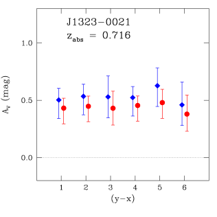
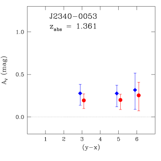
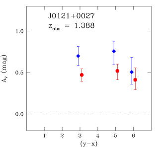
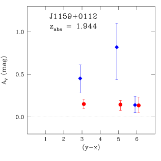
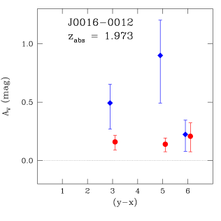
Figure 2: Extinction $A_{V}$ of the reddened quasars of Table 2 estimated in the rest frame of the intervening DLA system and plotted versus color index for different extinction curves. Color index coding: $1=(u\!-\!z)$, $2=(u\!-\!i)$, $3=(g\!-\!z)$, $4=(u\!-\!r)$, $5=(g\!-\!i)$; $6=(r\!-\!z)$. Circles: SMC extinction curve. Diamonds: MW extinction curve. See Section 3.1.

3.1 Conversion to rest-frame extinction

The quasar reddening measured in the observer’s frame, $\Delta(y-x)$, can be converted to the $V$ band extinction in the rest-frame of the absorber, $A_{V}$, if one knows the normalized extinction curve of the absorber, $\nobreak{\xi(\lambda)\equiv A_{\lambda}/A_{V}}$, and its redshift, $z_{\mathrm{abs}}$. In the Appendix A we show how to perform this conversion taking into account the slope of the quasar continuum. If the bandpasses are sufficiently narrow, the variation of the continuum accross the bandpass can be neglected. In this case, we obtain the simple relation useful for the purpose of discussion,

$$A_{V}\simeq{\Delta(y-x)\over\xi({\lambda_{y_{m}}\over 1\!+\!z_{\mathrm{abs}}})-\xi({\lambda_{x_{m}}\over 1\!+\!z_{\mathrm{abs}}})}\leavevmode\nobreak\ ,$$ (2)

where $\lambda_{x_{m}}$ and $\lambda_{y_{m}}$ are the wavelengths of maximum response of the bandpasses $x$ and $y$. The values of $A_{V}$ presented in our work, however, were derived from the more general relation (17) which is also valid for wide bandpasses. The response curves of the SDSS $ugriz$ bandpasses were taken from Fukugita et al. (1996 and priv. comm.). We adopted a power law with spectral index $\alpha_{\nu}=-0.5$ for the quasar continuum.

In our computations we used the two extinction curves most commonly adopted in the literature, i.e. the average curve of the Milky Way, characterized by an extinction bump at 217.5 nm and that of the Small Magellanic Cloud (SMC), characterized by a fast UV rise and without the bump (see e.g. Draine 2003). For the first one we adopted the model of Cardelli et al. (1988; CCM) with $R_{V}=3.1$. For the SMC curve we fitted the model of Pei (1992; hereafter P92) to the average SMC bar data of Gordon et al. (2003; hereafter G03). As we show in Fig. 1, the adopted MW and SMC curves are very similar to the models of P92 often used in the literature.

From previous studies we expect the incidence of MW curves to be very low, compared to that of SMC curves, among quasar absorbers (Wild & Hewett 2005; York et al. 2006 and refs. therein). However, in a few cases evidence for MW-type curves has been reported, with one clear detection of the bump in a DLA system at $z_{\mathrm{abs}}=0.524$ observed with the HST (Junkkarinen et al. 2004), and three possible identifications in absorption systems at $z_{\mathrm{abs}}\simeq 1.4$ - $1.5$ observed in SDSS quasar spectra (Wang et al. 2004).

In principle any type of extinction curve can be used in the conversion from reddening to rest-frame extinction. In practice, however, the results obtained from flat extinction curves, such as the MW curves with $R_{V}\raisebox{-5.0pt}{$\;\stackrel{{\scriptstyle\textstyle>}}{{\sim}}\;$}5$, are unreliable. This can be understood from the simple relation (2): if the extinction curve is exactly flat the measured $\nobreak{\Delta(y-x)}$ is divided by zero in the conversion.

3.2 Comparison of results obtained from different color indices

The rest frame extinction $A_{V}$ is an intrinsic property of the absorber and must be independent of the bandpasses $x$ and $y$ used in the measurement of the reddening. Therefore, by comparing values of $A_{V}$ obtained from different measurements of $\Delta(y-x)$ in the same quasar we can test the hypothesis that the measured reddening originates in the intervening system. If the hypothesis is correct, we must obtain a constant $A_{V}$ from the different values of $\Delta(y-x)$ converted using the redshift $z_{\mathrm{abs}}$ and the extinction curve $\xi(\lambda)$ of the absorber.

The result of this test depends on the adopted extinction curve. However, all known extinction curves share a very similar slope in the spectral region redwards of the $217.5$ nm bump (see Fig. 1). Therefore, when $z_{\mathrm{abs}}$ is sufficiently low for all the bandpasses to fall redwards of the redshifted bump the test is, in practice, independent of the adopted curve.

In Fig. 2 we plot $A_{V}$ versus color index for the average MW and SMC extinction curves. Only quasars for which the reddening was detected in at least three colors are shown in the figure. One can see in Fig. 2 that in each quasar $A_{V}$ is constant within the errors for at least one of the two extinction curves. The test is particularly stringent for J1323$-$0021, for which we have at our disposal 6 different measurements. These results are consistent with the hypothesis that the reddening originates in the intervening DLA systems.

As expected, the test is unable to discriminate between different types of extinction curves for the absorbers at lower redshift. However, when $z_{\mathrm{abs}}$ is sufficiently high to sample the far UV region of the extinction curve, the test can also be used to discriminate between different extinction curves. In fact, for the two absorbers at $z_{\mathrm{abs}}\sim 2$ towards J1159+0112 and J0016-0012 the test favours an extinction curve of SMC type which, at variance with the MW curve, yields a constant $A_{V}$ from the different measurements of $\Delta(y-x)$ (bottom panels in the figure).

In principle, the comparison of the results obtained from different color indices could also be used to test whether the absorber originates at the redshift of the quasar or not. We have performed this test for the cases in which $z_{\mathrm{qso}}$ is significantly larger than $z_{\mathrm{abs}}$, namely J1323$-$0021, J2340$-$0053 and J0121+0027. In all these cases we find that a MW-type extinction curve does not pass the test ($A_{V}$ shows a large scatter in different color indices), but an SMC extinction curve is still a viable possibility ($A_{V}$ is approximately constant). We conclude that this test, taken alone, is unable to rule out the possibility that the reddening originates at the redshift of the quasar. This in turn implies that the reddening detection, even if confirmed in different color indices, must be accompanied by a spectroscopic analysis of the absorption lines, in order to establish the location along the line of sight of the absorber responsible for the reddening. This conclusion is reinforced by the analysis of the quasars without absorption lines in our control samples: by choosing very reddened quasars in these samples one may obtain an approximately constant $A_{V}$ adopting an arbitrary value of $z_{\mathrm{abs}}<z_{\mathrm{qso}}$ in the conversion from reddening to extinction.

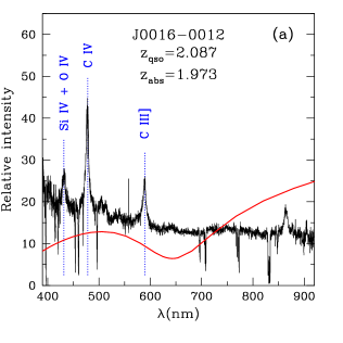
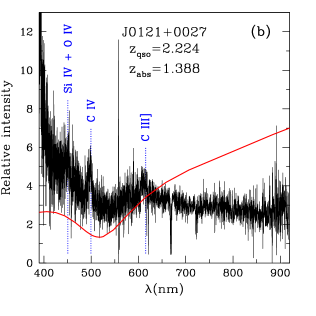
Figure 3: SDSS spectra of two quasars with a foreground DLA system at redshift $z_{\mathrm{abs}}$. Smooth lines: MW-type extinction curve ($R_{V}=3.1$) plotted in a scale $\nobreak{10^{-\xi[\lambda/(1+z_{\mathrm{abs}})]}}$. See Section 3.3. The predicted positions of some emission lines typical of quasar spectra are indicated. Intensities are in arbitrary units.

3.3 Extinction curve and average $A_{V}$

In order to obtain a value of $A_{V}$ for each absorption system of our sample we adopted one of the two types of extinction curve (SMC or MW) and then averaged the extinction obtained from different color indices. In practice, we averaged the independent measurements of $A_{V}$ obtained from two colors without common passbands. Local systematic errors, such as the contamination of the quasar continuum by emission lines, are minimized in this way. In most cases, we averaged the measurements obtained from the $(g-i)$ and $(r-z)$ colors. For the quasars with $u$ band not contaminated by Ly $\alpha$ emission/forest ($z_{\mathrm{qso}}<1.67$) we used the $(u-i)$ and $(g-z)$ colors, which have a larger spectral leverage for the detection of the reddening. For J2234+0000 ($z_{\mathrm{qso}}=3.015$) we only had one uncontaminated color index, i.e. the $(r-z)$.

In order to choose the extinction curve we analysed the SDSS spectra of the quasars of our sample in a search for the redshifted 217.5 nm extinction bump. Since this feature is present in the MW curve but absent in the SMC curve, it can be used to discriminate between the two types of extinction. Within the limits of the wavelength coverage of the SDSS spectra we were able to search for the redshifted bump in 8 quasars of our list.

In 7 of these quasars we do not find evidence of the bump from the comparison of the quasar spectrum with the MW-type extinction curve (CCM with $R_{V}=3.1$) plotted in a scale $\nobreak{10^{-\xi[\lambda/(1+z_{\mathrm{abs}})]}}$ which, apart from a constant factor, represents the transmission of the DLA system (see Eq. 13 in Appendix A). One example of negative detection is shown in Fig. 3a, where one can see that the continuum of J0016-0012 changes smoothly, as expected by a power law, in the region where the bump is expected to produce a broad, deep absorption. We cannot exclude that, in exceptional cases, a particular combination of quasar emission lines may conspire to hide a dust bump, if present. However, it is unlikely that this happens systematically in the 7 cases considered here, characterized by different combinations of emission and absorption redshifts. In particular, we do not find the bump in J1159+0112 and J0016-0012, the two cases for which the test of Fig. 2 indicates an SMC type extinction. In these two cases, therefore, we have two tests, one based on photometry and the other on spectroscopy, that consistently suggest an SMC-type extinction curve.

Only in one case, J0121+0027, we found tentative evidence of the bump. This case is shown in Fig. 3b, where one can see that the continuum of J0121+0027 runs smoothly at $\lambda>600\,\mathrm{nm}$, but shows an absorption at $400\,\mathrm{nm}\raisebox{-5.0pt}{$\;\stackrel{{\scriptstyle\textstyle<}}{{\sim}}\;$}\lambda\raisebox{-5.0pt}{$\;\stackrel{{\scriptstyle\textstyle<}}{{\sim}}\;$}600\,\mathrm{nm}$. The position, width and intensity of this absorption feature are broadly consistent with those predicted for the bump, given the uncertainties induced by the quasar emission lines. For this absorber we consider the possibility that the extinction curve may be of Milky-Way type, without ruling out completely a SMC-type curve (see Table 3). We refer to Wang et al. (2004) for a detailed spectroscopic analysis of this case.

For the absorbers of our list without spectral coverage of the bump we adopted an SMC curve. This choice is justified by the results of Wild & Hewett (2005) and York et al. (2006) which have found no evidence of the bump in their average absorber spectra. In any case, the results for an SMC and MW curve are often very similar. For the DLA system in front of J1323$-$0021, the only reddened quasar of our list without adequate spectral coverage of the bump, we expect a difference of only 0.08 dex in $A_{V}$.

The resulting values of extinction are listed in Table 3. The large upper error bar that we assign to J0121+0027 reflects the uncertainty in the choice of $R_{V}$, since a value as high as $R_{V}\sim 5.5$ has been proposed by Wang et (2004) for the absorber at $z_{\mathrm{abs}}=1.388$ (see footnote $h$). If $R_{V}$ is so high, the extinction curve becomes flat and the conversion from reddening to $A_{V}$ unreliable, as we explained above. In any case the value of extinction inferred by Wang et al. for this system, $\log A_{V}\simeq+0.10$ dex, lies well within our upper error bar.

Table 3: Extinction and metal column densities of the DLA systems of Table 1.

SDSS	$z_{\mathrm{abs}}$	$\langle\log A_{V}\rangle^{a}$	$(\log A_{V})^{b}_{\mathrm{pred}}$	$\log N({Zn\textsc{ii}})^{c}$	[Zn/Fe]c	$(\log\widehat{N}_{\mathrm{Fe}})^{d}$	$(\log\widehat{N}_{\mathrm{Fe}})^{e}$	$(\log\widehat{N}_{\mathrm{Fe}})^{f}$
J0013+0004	2.025	$<-1.02$	$-1.89,-1.67$	$12.25\pm 0.05$	$0.05\pm 0.07$	$<15.00^{g}$	$<15.00^{g}$	$<14.80^{g}$
J0016-0012	1.973	$-0.80_{-0.21}^{+0.11}$	$-1.22,-1.00$	$12.82\pm 0.04$	$0.84\pm 0.05$	$15.61\pm 0.04$	$15.62\pm 0.04$	$15.50\pm 0.04$
J0121+0027h	1.388	$-0.16_{-0.15}^{+0.76}$	—	$>13.32$	$>1.48$	$>16.17$	$>16.44$	$>16.19$
J0938+4128	1.373	$<-0.69$	$-1.85,-1.63$	$12.25\pm 0.05$	$0.29\pm 0.11$	$14.80\pm 0.14$	$14.80\pm 0.14$	$14.56\pm 0.14$
J0948+4323	1.233	$<-0.51$	$-1.03,-0.80$	$13.15\pm 0.01$	$0.45\pm 0.02$	$15.82\pm 0.02$	$15.82\pm 0.02$	$15.65\pm 0.02$
J1010+0003	1.265	$<-0.88$	$-0.98,-0.76$	$13.15\pm 0.06$	$0.75\pm 0.08$	$15.93\pm 0.06$	$15.93\pm 0.06$	$15.80\pm 0.06$
J1107+0048	0.741	$<-0.58$	$-1.01,-0.79$	$13.03\pm 0.05$	$0.37\pm 0.08$	$15.65\pm 0.08$	$15.65\pm 0.08$	$15.46\pm 0.11$
J1159+0112	1.943	$-0.85_{-0.22}^{+0.10}$	$-1.25,-1.02$	$13.09\pm 0.08$	$0.45\pm 0.11$	$15.76\pm 0.10$	$15.76\pm 0.10$	$15.59\pm 0.12$
J1232$-$0224	0.395	$<-0.50$	$-1.10,-0.87$	$12.93\pm 0.12$	$0.83\pm 0.16^{k}$	$15.72\pm 0.12$	$15.72\pm 0.12$	$15.60\pm 0.13$
J1323$-$0021	0.716	$-0.36_{-0.12}^{+0.07}$	$-0.56,-0.33$	$13.43\pm 0.05$	$1.14\pm 0.06$	$16.26\pm 0.05$	$16.28\pm 0.05$	$16.16\pm 0.05$
J1501+0019	1.483	$<-0.79$	$-0.92,-0.70$	$13.10\pm 0.05$	$0.40\pm 0.09^{k}$	$15.74\pm 0.08$	$15.74\pm 0.08$	$15.56\pm 0.11$
J2234+0000	2.066	$<-0.61$	$-1.60,-1.38$	$12.46\pm 0.02$	$0.57\pm 0.06$	$15.19\pm 0.03$	$15.19\pm 0.03$	$15.05\pm 0.04$
J2340$-$0053	1.360	$-0.67_{-0.32}^{+0.11}$	—	$12.62\pm 0.05$	$0.54\pm 0.13$	$15.33\pm 0.07$	$15.33\pm 0.07$	$15.18\pm 0.10$

^a Measured from the observed reddening using Eq. (17) for the conversion to rest frame extinction.
^b Extinction predicted from Eq. (11) of Vladilo & Péroux (2005) for $G=0.6$ and $G=1$, respectively.
^c See references in Table 1.
^d Calculated assuming Zn completely undepleted and [Zn/Fe]${}_{a}=0$.
^e Calculated using a scaling law of interstellar depletions (Vladilo 2002b; $\epsilon_{\mathrm{Zn}}=1$, $\eta_{\mathrm{Zn}}=42.5$) and [Zn/Fe]${}_{a}=0$.
^f As in the previous column, but with [Zn/Fe]${}_{a}=+0.1$ dex.
^g Dust-free system; upper limit computed introducing $\log N({Zn\textsc{ii}})<12.40$ and $\log N({Fe\textsc{ii}})>14.91$ in Eqs. (5) and (4).
^h Central and upper values of $\langle\log A_{V}\rangle$ calculated using a CCM model with $R_{V}=3.1$ and $R_{V}=5.5$, respectively. Lower value calculated using the SMC extinction curve (see Section 3.1).
^k $N$(Ni) or $N$(Cr) used as a proxy of $N$(Fe), which is not measured; Ni and Cr are good tracers of Fe in stars with [Fe/H] $\raisebox{-5.0pt}{$\;\stackrel{{\scriptstyle\textstyle>}}{{\sim}}\;$}-2$ dex (e.g. Ryan et al. 1996); Ni, Cr and Fe have very similar interstellar depletions (e.g. Vladilo 2002a); we adopt [Ni/Fe]=0 and [Cr/Fe]=0 in the conversion.

4 Extinction versus metal column density

On the basis of the of the selection process of our sample (Section 2) we assume that the DLA systems of Table 1 are the major source of reddening of their quasars and we investigate the relation between the quasar extinction and the DLA metal column density. The rest-frame extinction scales with the dust-phase column density of iron, $\widehat{N}_{\mathrm{Fe}}$ [cm^-2], according to the relation

$$A_{V}=\,\,\langle s^{\mathrm{Fe}}_{V}\rangle\leavevmode\nobreak\ \widehat{N}_{\mathrm{Fe}}\leavevmode\nobreak\ ,$$ (3)

derived in Appendix B. The term $\langle s^{\mathrm{Fe}}_{V}\rangle$ is the mean optical cross section of the dust grains in the $V$ band per atom of iron in the dust. The extinction will change between different lines of sight tracking the variations of the dust-phase column density of iron and of the mean cross section $\langle s^{\mathrm{Fe}}_{V}\rangle$. Our goal is to probe the behaviour of $\langle s^{\mathrm{Fe}}_{V}\rangle$ in different H i regions from a simultaneous measurement of $A_{V}$ and $\widehat{N}_{\mathrm{Fe}}$. The measurement of $\widehat{N}_{\mathrm{Fe}}$ in extragalactic clouds is discussed in the next section.

4.1 The dust-phase column density of iron

The dust-phase column density of iron cannot be measured directly from optical/UV spectroscopic data. With this type of observations, however, we can infer $\widehat{N}_{\mathrm{Fe}}$ from the measured gas-phase column densities of zinc and iron. We use zinc as gas-phase tracer of iron, since zinc is a volatile element with little affinity to dust (Savage & Sembach 1996) and, at the same time, the zinc/iron abundance ratio is approximately constant, in solar proportion, in a large fraction of Galactic stars over a very wide range of metallicities (Mishenina et al. 2002, Gratton et al. 2003, Nissen et al. 2004).

If zinc were completely undepleted and the intrinsic Zn/Fe ratio in DLA systems perfectly solar, the Zn/Fe ratio observed in the gas would give an exact measure of the iron depletion $\delta_{\mathrm{Fe}}\equiv\log(N_{\mathrm{Fe}}/N_{\mathrm{Zn}})-\log\mathrm{(Fe/Zn)}_{\sun}$. In this case the dust-phase column density of iron would be

$$\widehat{N}_{\mathrm{Fe}}=f_{\mathrm{Fe}}\,N_{\mathrm{Zn}}\,\left({{\mathrm{Fe}\over\mathrm{Zn}}}\right)_{\!\sun}\leavevmode\nobreak\ ,$$ (4)

where $f_{\mathrm{Fe}}=1-10^{\delta_{\mathrm{Fe}}}$ is the fraction of iron in the dust. With this expression $\widehat{N}_{\mathrm{Fe}}$ can be directly estimated from the measured column densities $N_{\mathrm{Zn}}$ and $N_{\mathrm{Fe}}$.

A closer inspection of interstellar data, however, indicates that zinc also can be depleted, with an extreme value as high as $-0.6$ dex in dense clouds such as that in front of $\zeta$ Oph (Savage & Sembach 1996). Therefore, we must take into account the possibility that zinc may also be depleted (in small amounts) in DLA systems.

In addition, a closer analysis of stellar data shows that the Zn/Fe ratio tends to increase with decreasing metallicity. The effect is strong when [Fe/H] $<-2$ dex, attaining a value as high as [Zn/Fe] $\simeq+0.5$ dex at [Fe/H] $\sim-4$ dex (Cayrel et al. 2004). Luckily, this interval of metallicities is well below the typical metallicities of DLA systems. However, a mild excess has also been found in a fraction of Galactic stars which are less metal deficient (Prochaska et al. 2000, Chen et al. 2004). For stars of the thin disk the typical excess is [Zn/Fe] $\simeq+0.1$ dex at [Fe/H] = $-0.6$ dex and vanishes at higher metallicities (Chen et al. 2004).

By allowing a fraction $f_{\mathrm{Zn}}$ of zinc to be in the dust and the intrinsic Zn/Fe ratio of the absorbers, $\left({\mathrm{Zn}\over\mathrm{Fe}}\right)_{a}$, to deviate from the solar value, we obtain the more general expression

$$\widehat{N}_{\mathrm{Fe}}=f_{\mathrm{Fe}}\,{N_{\mathrm{Zn}}\over(1-f_{\mathrm{Zn}})}\,\left({\mathrm{Zn}\over\mathrm{Fe}}\right)^{-1}_{a}\leavevmode\nobreak\ .$$ (5)

With an educated guess of $\mathrm{(Zn/Fe)_{a}}$ it is possible to estimate $\widehat{N}_{\mathrm{Fe}}$ from the column densities $N_{\mathrm{Zn}}$ and $N_{\mathrm{Fe}}$ also in this general case, assuming that $f_{\mathrm{Zn}}$ scales with $f_{\mathrm{Fe}}$ according to a scaling law of interstellar depletions calibrated in the ISM. Details on this method can be found in Vladilo (2002a, 2002b).

In Table 3 we give the dust-phase column densities of iron calculated for three different cases: (1) zinc completely undepleted and $\mathrm{[Zn/Fe]_{a}}=0$ (column 7); (2) zinc depletion scales with iron depletion and $\mathrm{[Zn/Fe]_{a}}=0$ (column 8); (3) zinc depletion scales with iron depletion and $\mathrm{[Zn/Fe]_{a}}=+0.1$ (column 9).

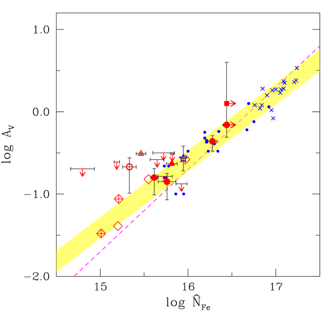
Figure 4: Extinction, $A_{V}$, versus dust-phase column density of iron, $\widehat{N}_{\mathrm{Fe}}$, in QSO absorbers and interstellar clouds. The extinction is calculated in the rest frame of the absorber. Circles and arrows pointing down: $A_{V}$ measurements and upper limits from this work; empty circle: J2340$-$0053. Triangles: QSO/DLAs from Ellison et al. (2005); empty triangle: B0438$-$436. Square: extinction for J0121+0027 from Wang et al. (2004). Crossed diamonds: sub-samples of Mg ii absorbers from York et al. (2006). Open diamonds: sub-samples of Ca ii absorbers from Wild et al. (2006). Open star: SMC line of sight towards Sk 155 (Welty et al. 2001, Fitzpatrick 1985). Dots and crosses: Milky Way interstellar lines of sight from Jenkins et al. (1986) and Snow et al. (2002), respectively. Strip: $\pm 1\,\sigma$ interval around the linear regression of the MW data. Dashed line: linear regression of the MW data with fixed unit slope. See Sect. 4.2.

The comparison between columns 7 and 8 indicates that the results are almost unaffected by the possible depletion of zinc. Only when the depletion level is particularly high, i.e. when [Zn/Fe] $\;\stackrel{{\scriptstyle\textstyle>}}{{\sim}}\;$ 1 dex, the correct relation (5) yields slightly higher values of $\widehat{N}_{\mathrm{Fe}}$ than the approximate relation (4).

The comparison between columns 8 and 9 indicates that a mild excess of the intrinsic abundance ratio $\mathrm{[Zn/Fe]_{a}}$ yields a similar mild decrease of $\widehat{N}_{\mathrm{Fe}}$ with respect to the case $\mathrm{[Zn/Fe]_{a}}=0$. The higher the observed [Zn/Fe] ratio, the lower the difference. For the quasars with reddening detection the observed [Zn/Fe] ratio of the DLA happens to be relatively high (column 4 in Table 3). Therefore the results of the present work are weakly affected by an excess of $\mathrm{[Zn/Fe]_{a}}$ of the type observed in stars of moderately low metallicity.

In fact, for two of the quasars with reddening detection (J0121+0027 and J1323$-$0021) the metallicity of the intervening DLA system is relatively high (Wang et al. 2004, Péroux et al. 2006) and we do not expect an excess of $\mathrm{[Zn/Fe]_{a}}$ given the trend of [Zn/Fe] observed in Galactic stars (Chen et al. 2004). The absorber with lowest metallicity among the 5 quasars with reddening detection is that at $z_{\mathrm{abs}}=1.944$ towards J1159+0012 ([Zn/H] $\simeq-1.4$ dex). This is the absorber in which $\mathrm{[Zn/Fe]_{a}}$ could be, in principle, most enhanced. As we show below, the results of this paper are unaffected even in this case.

4.2 The empirical relation between $A_{V}$ and $\widehat{N}_{\mathrm{Fe}}$

In Fig. 4 we plot the rest frame extinction, $A_{V}$, versus the dust-phase column density of iron, $\widehat{N}_{\mathrm{Fe}}$, for different types of absorbers of the local and high redshift Universe.

The data obtained from our reddening detections at the $\nobreak{2\,\sigma}$ level are indicated with circles. The filled circles are the quasars in which the DLA system of Table 1 is the major source of reddening. The empty circle is J2340-0053, for which an additional contribution to the reddening may be present. For J0121+0027 we also plot the extinction derived by Wang et al. (2004) from the comparison with composite SDSS quasar spectra (filled square).

For the cases without reddening detection we plot a 2 $\sigma$ upper limit. The values of $\widehat{N}_{\mathrm{Fe}}$ are estimated from Eq. (5), case [Zn/Fe]_a=0. The implications of these choices are discussed below.

The triangles in the figure represent two quasars with photometric reddenings and DLA metal column densities obtained in the framework of the CORALS survey (Ellison et al. 2005). These quasars are not included in SDSS catalog. To estimate $A_{V}$ we adopted the normalized colour $(B-K)_{n}$ in Table 3 of Ellison et al. and an SMC extinction curve. Only two quasars of this survey (B0438$-$436 and B0458$-$020) have a significant $(B-K)$ reddening and, at the same time, Zn and Fe column densities (Akerman et al. 2005). The quasar B0438$-$436 is represented with an empty triangle, rather than a filled one, because its reddening seems to be contaminated by dust in the quasar environment (Ellison et al. 2005).

The crossed diamonds in the figure are taken from a study of the average reddening properties of 809 Mg ii systems in SDSS quasar spectra (York et al. 2006). The redshift interval covered by this study is similar to that of the DLA systems of Table 1. However, Mg ii absorbers may have, in general, H i column densities well below the DLA regime. For comparison with our data we have considered the sub-samples of York et al. with largest equivalent widths of Mg ii because in these sub-samples the fraction of DLA systems is expected to be the highest. The results shown in the figure represent the mean values of $A_{V}$ and $\widehat{N}_{\mathrm{Fe}}$ for the sub-samples S8 (251 systems with equivalent widths $>$ 2 Å) and S26 (97 systems with equivalent widths $>$ 2.5 Å and $\Delta(g-i)<0.2$ magnitudes). Sub-samples with saturated Zn ii and Fe ii mean profiles were not considered. The mean extinction was estimated from the mean $E(B\!-\!V)$ of these sub-samples using the SMC value $R_{V}=2.74$ (Gordon et al. 2003). The mean $\widehat{N}_{\mathrm{Fe}}$ was derived by inserting the mean $N({Zn\textsc{ii}})$ and [Zn/Fe] of the sub-samples in relation (5).

The open diamonds are taken from the study of Ca ii systems at $z\sim 1$ in SDSS quasar spectra by Wild et al. (2006). In order of increasing extinction, they represent the mean values of $A_{V}$ and $\widehat{N}_{\mathrm{Fe}}$ for the sub-samples labelled Low-$W_{\lambda 3935}$, All, and High-$W_{\lambda 3935}$, respectively. We estimated these mean values from the corresponding mean values of $E(B\!-\!V)$, $N({Zn\textsc{ii}})$ and [Zn/Fe] given by Wild et al. (2006) for the 27 absorbers analysed for element column densities. Also in this case we assume an SMC type of dust.

The quasar absorption data in Fig. 4 are consistent with an increase of $A_{V}$ with increasing $\widehat{N}_{\mathrm{Fe}}$. A linear trend between these two quantities is predicted by relation (3) if the mean extinction per atom of iron is approximately constant in H i interstellar regions. However, the number of data points for the individual quasar absorbers (circles and triangles) is too little for deriving a statistical correlation. In order to cast light on the behaviour of high redshift clouds we added in the same figure results obtained for local interstellar clouds.

The dots and crosses in the figure represent Milky-Way lines of sight with available measurements of $A_{V}$, $N(\mathrm{H_{tot}})=N({H\textsc{i}})+2N(\mathrm{H}_{2})$ and $N({Fe\textsc{ii}})$, taken from Jenkins et al. (1986) and Snow et al. (2002), respectively. For these data we derived $\widehat{N}_{\mathrm{Fe}}$ assuming that the local interstellar abundance of iron is solar. The error budget in the estimate of $\widehat{N}_{\mathrm{Fe}}$ is dominated by the error of $N(\mathrm{H_{tot}})$, which is typically of $\sim 0.1$ dex. The extinctions were taken from the catalog of Neckel & Klare (1980), under the entry $A_{V}$(MK). Uncertainties of these $A_{V}$ values are in the order of 0.1 mag. Values with $A_{V}<0.1$ mag were not considered. Lines of sight with $N({H\textsc{i}})$ below the definition threshold of DLA systems and with saturated iron lines were rejected.

The Milky-Way data are highly correlated, with linear correlation coefficient $r=0.95$ and slope $m=0.81\pm 0.27$. The strip in the figure represents the dispersion of the data around the linear regression. The dashed line is the linear regression with fixed $m=1$, a slope consistent with the free regression analysis.

The star symbol in the figure represents the SMC star Sk 155, the only Magellanic sightline for which we could determine $A_{V}$ and $\widehat{N}_{\mathrm{Fe}}$. The extinction was estimated using the SMC value of $E(B\!-\!V)$ from Fitzpatrick (1985) and the mean SMC value $R_{V}=2.74$ (Gordon et al. 2003). We estimated $\widehat{N}_{\mathrm{Fe}}$ from relation (5) using the Zn and Fe column densities of Welty et al. (2001) integrated over the SMC radial velocities. In spite of the differences in metallicity level and type of extinction curve relative to the Milky Way, the data point of Sk 155 is in excellent agreement with the Milky-Way data.

Most of the DLA measurements (filled circles and triangles) follow the trend of Milky-Way interstellar data. Uncertainties in the choice of the extinction curve are unlikely to alter this result. Even in the case of J0121+0027, for which these uncertainties are large, the DLA data point seems to be consistent with the interstellar trend (the value of $\widehat{N}_{\mathrm{Fe}}$ is a lower limit owing to saturation of the Zn ii lines).

Also the uncertainty in the adopted value of $\nobreak{\mathrm{[Zn/Fe]}_{a}}$ in Eq. (5) is unlikely to affect the agreement between DLA systems and interstellar clouds. As we said above, J1159+0112 is the most likely candidate for a mild enhancement of $\nobreak{\mathrm{[Zn/Fe]}_{a}}$ among our quasars with reddening detection. By adopting an enhanced [Zn/Fe]_a in this case (last column of Table 3), we still find a good agreement with the Milky-Way data.

In spite of this general agreement, an excess of extinction relative to the Milky-Way trend is found in J2340-0053 (empty circle) and B0438-436 (empty triangle). Quite interestingly, these are exactly the cases for which we suspect the presence of extinction sources in addition to the DLA system. Therefore, the excess may be due to the presence of additional absorbers rather than to a deviation of individual DLAs from the interstellar trend.

Also the $A_{V}$ upper limits that we derive are generally consistent with the interstellar data. This conclusion would be strengthened by adopting an enhanced [Zn/Fe]_a in Eq. (5), instead of $\nobreak{\mathrm{[Zn/Fe]}_{a}=0}$, since in this case the limits would shift slightly to the left (see Table 3).

In summary, the data collected in the figure suggest that the trend between $A_{V}$ and $\widehat{N}_{\mathrm{Fe}}$ is remarkably similar in interstellar clouds of the Milky Way and the SMC and in DLA systems with different metallicities (from $\simeq-1.4$ dex up to $\simeq+0.5$ dex relative to solar) and redshifts ($z\simeq 0.7$ up to $z\simeq 2$). Also Ca ii absorbers and the Mg ii absorbers with highest values of equivalent width follow the same trend.

In the interpretation of the results of Fig. 4 one must take into account that some parts of the plot are not accessible to the observations. For instance, if $A_{V}$ is too large, the background quasar drops out of the SDSS sample. If it is too low, the reddening cannot be detected. The detection limit, in addition, will vary as a function of the redshift and of the scatter of the intrinsic colors of the quasars. These effects may alter the distribution of detected DLA systems in Fig. 4 and, in principle, could induce an artificial trend among the data points.

The agreement between the different sets of high redshift data in Fig. 4 is impressive, considering the different methods employed for measuring the reddening. Also the agreement between high redshift and local data is remarkable, considering the different methods used to derive $A_{V}$ and $\widehat{N}_{\mathrm{Fe}}$ (for instance, the educated guess of [Zn/Fe]_a was applied to derive $\widehat{N}_{\mathrm{Fe}}$ at high redshift, but not in the Milky Way). The general agreement between DLA and interstellar data speaks against the existence of an artificial trend induced by selection effects of DLA detections. The implications of this general agreement are discussed below.

5 Discussion

5.1 Implications for the properties of dust grains

The existence of a common trend between $A_{V}$ and $\widehat{N}_{\mathrm{Fe}}$ in H i regions of galaxies with different metallicities and redshifts indicates that the dust grain parameter

$$\langle s^{\mathrm{Fe}}_{V}\rangle=1.007\!\times\!10^{-22}\leavevmode\nobreak\ {\sum_{j}w_{j}\,\langle\,Q_{\lambda_{V}}\leavevmode\nobreak\ \sigma_{g}\,\rangle_{j}\over\sum_{j}w_{j}\,\langle\,V_{g}\,\varrho\leavevmode\nobreak\ X_{\mathrm{Fe}}\,\rangle_{j}}$$ (6)

representing the mean extinction in the $V$ band per atom of iron in the dust (see Appendix B), is approximately constant in a large variety of neutral regions. The scatter of the Milky Way data is of only 0.16 dex at 1 $\sigma$ level. The few measurements in DLA systems do not show, so far, evidence for a larger dispersion.

In principle, the $V$ band could be less sensitive than other spectral bands to variations of the extinction properties of the grains. Notwithstanding, the small scatter of $\langle s^{\mathrm{Fe}}_{V}\rangle$ is rather remarkable given the fact that the value of this parameter is determined by at least 4 different properties of the grains: their size, $a$, internal density, $\varrho$, abundance by mass of iron inside the grain, $X_{\mathrm{Fe}}$, and extinction efficiency factor, $Q_{\lambda}$ , which is related to the geometrical and optical properties of the grains (Spitzer 1978). We know that these parameters vary among interstellar clouds. In particular, the variations of the extinction curves are attributed, in large part, to variations of the grain size distribution (Draine 2003). Therefore, in order to produce an approximately constant $\langle s^{\mathrm{Fe}}_{V}\rangle$ there must be a physical mechanism able to compensate the variations of the individual parameters that appear in the above expression. We tentatively propose the following mechanism based on heuristic considerations.

We consider two types of interstellar environments: (1) regions where grain destruction mechanisms are efficient and (2) clouds where the grains are protected from destruction. In the second case we expect that the grain size $a$ can be larger, on the average, and the volatile elements more easily incorporated into the grains than in the first case. The relative abundance of iron inside the grains, $X_{\mathrm{Fe}}$, must be lower in the second case, when also volatile elements are incorporated in the grains, than in the first case, when refractory elements, such as iron, are dominant. Since the most abundant volatile elements (e.g. carbon) are lighter than the most abundant refractory elements (e.g. iron) we expect, in addition, that in the second case the mean density $\varrho$ is lower than in the first case.

Combining all together, we expect the following variations of the grain parameters to occur passing from a grain-destructive to a non-destructive environment: an increase of $a$ and, at the same time, a decrease of $\varrho$ and $X_{\mathrm{Fe}}$. From relation (6) we expect that $\langle s^{\mathrm{Fe}}_{V}\rangle\approx(a\,\varrho\,X_{\mathrm{Fe}})^{-1}$ since $\sigma_{g}\approx a^{2}$ and $V_{g}\approx a^{3}$. Given this dependence of $\langle s^{\mathrm{Fe}}_{V}\rangle$, the changes of $a$ could compensate the changes of $\varrho$ and $X_{\mathrm{Fe}}$.

A much larger database of interstellar data at low and high redshift are required to understand the viability of the simple mechanism of compensation proposed here. Contraints on this mechanism could be obtained by studying the slope of the $A_{V}$ and $\widehat{N}_{\mathrm{Fe}}$ relation and analysing possible variations of $\langle s^{\mathrm{Fe}}_{V}\rangle$ versus $R_{V}$. Given the paucity of quasar absorption extinction measurements these studies are still premature at high redshift, but could be the subject of future investigations.

5.2 Implications for the dust obscuration bias

The extinction of the quasars due to the intervening DLA systems is expected to produce a selection effect in optical, magnitude-limited surveys: the absorbers with highest values of extinction would be systematically missed from the surveys as a consequence of quasar obscuration (Fall & Pei 1989).

Evidence for this effect has been searched by comparing the statistics of optical surveys and radio-selected surveys, the latter being unaffected by the extinction. A marginal signature of the bias has been found in this way (Ellison et al. 2001, Akerman et al. 2005), but the statistics are still based on small numbers and the estimate of the effect uncertain due to the difficulty of observing all the quasars of the radio-selected sample, independently of their magnitude, in the optical follow-up.

In a previous work we have proposed a new approach for quantifying the effect of quasar obscuration on the statistics of DLA systems. Using a relation between the extinction and the metal column densities of the absorbers we invert the frequency distributions of H i column densities and metallicities measured from magnitude-limited surveys and derive the unbiased frequency distributions (Vladilo & Péroux 2005). The existence of a general relation between extinction and metal column density is fundamental in this type of approach. The results of the present work lend quantitative support to the relation adopted in our previous work, $\nobreak{A_{V}\simeq 1.85\times 10^{-14}\,G\,f_{\mathrm{Fe}}(Z)\,N_{\mathrm{H}}\,Z}$, which was mostly based on interstellar data. In Table 3, Col. 4, we list the values of extinction predicted from this previous relation for the DLA systems of the present work. One can see that the predictions are in most cases consistent with the measurements or upper limits. The agreement with the measurements is better for $G=1$ than for $G=0.6$ (in this latter case the extinction is mildly underestimated). These results indicate that the quantitative predictions of the obscuration bias presented by Vladilo & Péroux (2005) are realistic and, in any case, not overestimated.

In order to confirm the general validity of the relation between extinction and metal column densities in DLA systems, it would be important to obtain more measurements at higher redshifts since the present sample is limited at $z_{\mathrm{abs}}\simeq 2$, while a large fraction of DLA systems is observed to be at higher redshift. In particular, it will be crucial to calibrate the relation at high values of extinction ($A_{V}>1$ mag), when the obscuration bias is most critical. The slope $m\simeq 0.8$ of the interstellar data is consistent with a mild decrease of the extinction per atom of iron in the dust with increasing metal column density (strip in Fig. 4). For an exact estimate of the obscuration bias it is critical to verify the existence of this effect in DLA systems.

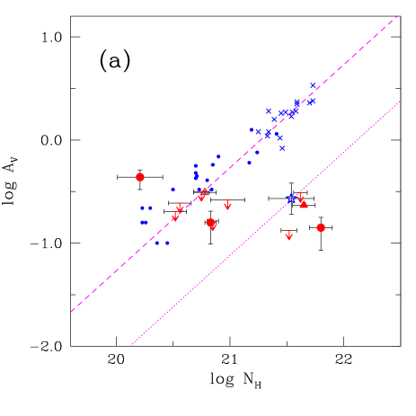
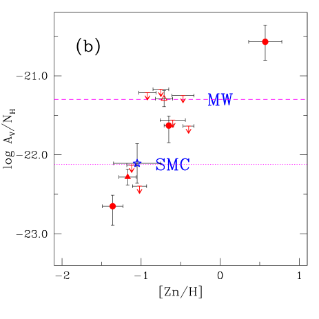
Figure 5: (a) Extinction, $A_{V}$, versus total hydrogen column density, $N_{\mathrm{H}}$, of DLA systems and interstellar clouds. Same symbols as in Fig. 4. Dashed line: mean MW $A_{V}/N_{\mathrm{H}}$ ratio for $R_{V}=3.1$ (Bohlin et al. 1978). Dotted line: mean SMC $A_{V}/N_{\mathrm{H}}$ ratio (Gordon 2003). (b) Dust-to-gas ratio, $A_{V}/N_{\mathrm{H}}$, versus metallicity for the same set of data. The labels indicate the regions of the diagram occupied by MW and SMC interstellar clouds.

5.3 The dust-to gas ratio $A_{V}/N_{\mathrm{H}}$

In Fig. 5a we plot $A_{V}$ versus the total hydrogen column density for the same data set of Fig. 4. For DLA absorbers we assume that $N_{\mathrm{H}}=N({H\textsc{i}})$, i.e. we neglect the molecular contribution. Two of our systems with reddening detections are not plotted because they do not have a direct determination of $N({H\textsc{i}})$ (see Table 1). This is also the case for the Mg ii absorbers of York et al. (2006) and the Ca ii absorbers of Wild et al. (2006) discussed in Section 4.2.

The comparison with the interstellar data shows that DLA systems do not follow the typical Milky Way relation of Bohlin et al. (1978), shown as a dashed line in the figure. Most systems lie below the MW trend and the addition of a molecular contribution to the hydrogen column density would not change this conclusion.

The analysis of the data versus metallicity reveals the existence of a regular behaviour. This can be seen in Fig. 5b, where we plot the dust-to-gas ratio $A_{V}/N_{\mathrm{H}}$ versus metallicity [Zn/H] for the same systems. In spite of the limited size of the DLA sample, the data suggest the existence of a trend of increasing dust-to-gas ratio with increasing metallicity. The trend nicely fits the regions of the diagram occupied by MW and SMC interstellar clouds, suggesting its general validity at low and high redshift.

The observed trend can be interpreted as a natural consequence of the approximate constancy of $\langle s^{\mathrm{Fe}}_{V}\rangle$ discussed above. In fact, dividing both sides of Eq. (3) by $N_{\mathrm{H}}$ and inserting relation (5), we obtain

$${A_{V}\over N_{\mathrm{H}}}=\langle s^{\mathrm{Fe}}_{V}\rangle\leavevmode\nobreak\ {f_{\mathrm{Fe}}\over(1-f_{\mathrm{Zn}})}\,{N_{\mathrm{Zn}}\over N_{\mathrm{H}}}\,\left({\mathrm{Zn}\over\mathrm{Fe}}\right)^{-1}_{a}\leavevmode\nobreak\ .$$ (7)

If $\langle s^{\mathrm{Fe}}_{V}\rangle$ is constant, we expect from this expression a linear trend between dust-to-gas ratio and metallicity (Zn/H), modulated by variations of the iron and zinc depletions; the intrinsic abundance ratio $\left({\mathrm{Zn}\over\mathrm{Fe}}\right)_{a}$ is not expected to show strong variations.

If the trends of Fig. 4 and 5 will be confirmed by a larger set of data, then it will be natural to explain the validity of the Bohlin et al. (1978) MW relation, $A_{V}/N_{\mathrm{H}}\sim$ constant, as the consequence of the constant metallicity level of MW clouds in conjunction with a constant $\langle s^{\mathrm{Fe}}_{V}\rangle$.

The deviations of the DLA dust-to-gas ratios from the Bohlin et al.’s value indicate that the MW ratio should not be applied to obtain indirect estimates of extinctions or $N_{\mathrm{H}}$ in extragalactic research. By taking into account the metallicity and the extinction curve of the absorbers one can, however, obtain reasonable estimates. Since quasar absorbers are, in general, metal deficient, the typical $A_{V}/N_{\mathrm{H}}$ ratio of the SMC (dotted line in Fig. 5) is more appropriate than the MW ratio for indirect estimates of extinctions or $N_{\mathrm{H}}$. The choice of an SMC dust-to-gas ratio is in line with the lack of 217.5 nm bump in most quasar absorbers (York et al. 2006).

6 Summary and conclusions

We have implemented a technique for measuring the reddening of quasars using the photometric and spectroscopic SDSS database. For each quasar under investigation we build up a control sample to analyse the distribution of the colors at a given redshift and magnitude. Quasars showing absorption lines redwards of the Ly $\alpha$ emission in their spectra are rejected from the control sample. The median and the dispersion of the color distribution are used to estimate the reddening and its uncertainty. To minimize systematic errors related to the presence of quasar emissions in particular passbands, the reddening is measured in different color indices.

We have applied this technique to the complete sample of 13 SDSS quasars for which a single intervening DLA system with zinc absorption lines had been previously detected in spectra of high (or intermediate) resolution. Most of the spectra of these quasars do not show evidence of potential sources of reddening other than the DLA systems. We detect reddening at the 2 $\sigma$ level in five of these quasars. In each case the detection is confirmed in different color indices. The comparison of the color excess measured in different pairs of bandpasses is consistent with an origin of the reddening in the DLA systems. To our knowledge this is the most direct evidence of DLA extinction up to $z\simeq 2$ obtained so far.

In order to discriminate the extinction curve of the absorbers we have compared the reddening in different color indices and investigated the region of the SDSS spectra where the redshifted 217.5 nm MW-extinction bump is expected to fall, if present. An SMC-type extinction curve is generally consistent with the available data, in agreement with previous studies of the extinction curves of Ca ii and Mg ii quasar absorbers (Wild & Hewett 2005, York et al. 2006). The only possible exception is J0121+0027, for which we cannot exclude that the MW bump is present, as claimed by Wang et al. (2004).

After converting the quasar reddening into $V$-band extinction in the rest frame of the DLA system, $A_{V}$ (see Appendix A), we have investigated the relation between $A_{V}$ and the dust-phase column density of iron of the absorber, $\widehat{N}_{\mathrm{Fe}}$. Our measurements and upper limits are consistent with a rise of $A_{V}$ with increasing $\widehat{N}_{\mathrm{Fe}}$, but the sample is too small to perform a correlation study.

By comparing these data with measurements of $A_{V}$ and $\widehat{N}_{\mathrm{Fe}}$ in Milky Way and SMC interstellar clouds, we obtain the main result of our work: the high-redshift data follow remarkably well the trend of the local interstellar data, which show a linear correlation $\log A_{V}$ - $\log\widehat{N}_{\mathrm{Fe}}$. Only in one quasar, J2340$-$0053, do we find an excess of extinction, possibly due to neutral gas at a redshift different from that of the DLA system.

Consistent results are found from the analysis of the two quasars with $(B-K)$ reddening detections recently reported by Ellison et al. (2005): one DLA system with Zn ii lines follows the Milky-Way trend and another one, towards B0438$-$436, shows an excess of extinction. In this case the excess is likely to originate in dust of the quasar environment (Ellison et al. 2005).

Finally, from the studies of Wild et al. (2006) and York et al. (2006), we find evidence that also the Ca ii quasar absorbers at $z\sim 1$ and the Mg ii absorbers with highest equivalent widths, statistically more similar to DLA systems, follow the interstellar trend between extinction and dust-phase metal column density.

The existence of a linear relation between $A_{V}$ and $\widehat{N}_{\mathrm{Fe}}$ shared by high redshift DLA galaxies and by local clouds of the Milky Way and the SMC suggests that the mean extinction per atom of iron in the dust, $\langle s^{\mathrm{Fe}}_{V}\rangle$, is approximately constant in galaxies with different levels of metallicity (from [Zn/H]$\simeq-1.4$ dex up to $\simeq+0.5$ dex) and look-back times (up to $\sim 10$ billon years before the present). This result in turn suggests the existence of a mechanism which tends to compensate variations of $\langle s^{\mathrm{Fe}}_{V}\rangle$ resulting from changes of the dust grain properties in different interstellar environments. We propose that when the grain size $a$ increases, the density of the grain, $\varrho$, and the abundance by mass of iron in the dust, $X_{\mathrm{Fe}}$, decrease (and vice versa). These variations are expected to occur when passing from a dust-destructive to a dust-protected environment (and vice versa).

The existence of a well defined trend between metal column densities and extinction in DLA systems at different redshifts has important implications for quantifying the selection effect of quasar obscuration (Fall & Pei 1989). The results of the present analysis lend quantitative support to the estimates of DLA extinction performed in our previous study of the obscuration effect (Vladilo & Péroux 2005).

Finally, from the analysis of the dust-to-gas ratio $A_{V}/N_{\mathrm{H}}$ in the DLAs of our sample, we find significant deviations from the Milky-Way ratio $A_{V}/N_{\mathrm{H}}\approx 5.3\times 10^{-22}$ mag cm² of Bohlin et al. (1978). The dust-to-gas ratio appears to increase with the metallicity of the absorber, following a trend that fits the SMC and MW data points, but more data are necessary to confirm this result. We argue that the constancy of the dust-to-gas ratio in local interstellar clouds is the result of their constant level of metallicity in conjunction with the lack of significant variations of $\langle s^{\mathrm{Fe}}_{V}\rangle$. The MW dust-to-gas ratio should not be used in extragalactic studies for indirect estimates of extinctions or H i column densities.

An important outcome of the present investigation stems from the comparison of the control samples before and after the rejection of quasars with absorptions lines redwards of the Ly $\alpha$ emission. After the rejection, the color distributions of the control samples experience a small but systematic blue shift indicating that these absorption lines do contribute to the reddening of quasars. This result is in line with the recent detection of reddening due to Ca ii (Wild & Hewett 2005, Wild et al. 2006) and Mg ii (Khare et al. 2005; York et al. 2006) absorption systems. Even in the absence of a direct measurement of the H i column densities of the Ca ii and Mg ii absorbers, the results of these previous investigations provide indirect evidence that DLA systems should give a signal of reddening. The present investigation is in line with this expectation, even if the sample is too small to draw general conclusions on the statistical properties of the extinction in DLA systems.

At the present state of the observations it is hard to understand whether or not there is a discrepancy between the reddening detection in Ca ii, Mg ii, and DLA absorbers at $z\raisebox{-5.0pt}{$\;\stackrel{{\scriptstyle\textstyle<}}{{\sim}}\;$}2$, on the one hand, and the upper limit found by Murphy & Liske (2004) in DLA systems at $z\sim 2.8$, on the other. Future studies of extinction and metal column densities in DLA systems should be aimed at obtaining measurements at higher redshifts ($z\raisebox{-5.0pt}{$\;\stackrel{{\scriptstyle\textstyle>}}{{\sim}}\;$}2$), at high values of extinctions ($A_{V}\raisebox{-5.0pt}{$\;\stackrel{{\scriptstyle\textstyle>}}{{\sim}}\;$}1$ mag) and at different values of $R_{V}$. With such measurements one should be able to understand if the relation between extinction and dust-phase metal column density is indeed universal, to probe the redshift evolution of the dust in cross-section selected galaxies, to quantify with accuracy the effect of quasar obscuration, and to probe the mechanism that makes $\langle s^{\mathrm{Fe}}_{\lambda}\rangle$ relatively constant in interstellar clouds.

Appendix A Conversion of the quasar reddening into rest frame extinction

Our goal is to estimate the rest frame extinction, $A_{V}$, from the measurement of the quasar reddening in the observer frame, $\Delta(y-x)$. We start from the definition of the apparent magnitude of a quasar in a photometric band $x$,

$$m_{x}=m_{x,\circ}\,-2.5\,\log\int_{\lambda_{x_{1}}}^{\lambda_{x_{2}}}\,F(\lambda)\,S_{x}(\lambda)\,d\lambda$$ (8)

where $m_{x,\circ}$ is the zero point of the photometric system; $F(\lambda)$ is the monochromatic flux of the quasar received out of the Earth’s atmosphere (erg s^-1 cm^-2 Å^-1); $S_{x}(\lambda)$ is the response curve of the passband $x$ (we include in this term the transmission of the Earth’s atmosphere and the response curve of the detector); $\lambda_{x_{1}}$ and $\lambda_{x_{2}}$ are the lower and upper cutoff of the bandpass.

The flux received at Earth from a quasar at redshift $z_{e}$ is

$$F(\lambda)={L({\lambda_{e}})H^{2}_{\circ}(1+z_{e})^{-3}\over 4\pi c^{2}Z^{2}_{q}(z_{e})}={L({\lambda_{e}})(1+z_{e})^{-1}\over 4\pi D_{L}^{2}}\;,$$ (9)

where the luminosity distance $D_{L}=c\,Z_{q}(z_{e})\,(1+z_{e})/H_{\circ}$ is defined through the function (Weinberg 1972)

$$Z_{q}(z_{e})={1\over q_{\circ}^{2}(1+z_{e})}\left\{q_{\circ}z_{e}+(q_{\circ}-1)\left[(1+2q_{\circ}z_{e})^{1\over 2}-1\right]\right\}.$$

Here $L(\lambda)$ is the monochromatic luminosity emitted by the quasar (erg s^-1 Å^-1), and $\lambda_{e}=\lambda/(1+z_{e})$.

From this we have

$$m_{x}=C_{x}(z_{e})-2.5\log\int_{\lambda_{x_{1}}}^{\lambda_{x_{2}}}\!\!L({\lambda_{e}})\,S_{x}(\lambda)\,d\lambda$$ (10)

where the term $C_{x}(z_{e})$ depends on the zero-point of the photometric system, the quasar redshift and the cosmological parameters.

We now consider the extinction due to an intervening interstellar medium $i$ that lies at the absorption redshift $z_{\mathrm{abs}}$ in the direction of the quasar. We call $S_{i}(\lambda)$ the transmission of the medium as a function of wavelength in the absorber rest frame [$S_{i}(\lambda)=1$ for a transparent medium]. The reddened magnitude of the quasar is

$$m^{\prime}_{x}=C_{x}(z_{e})-2.5\log\int_{\lambda_{x_{1}}}^{\lambda_{x_{2}}}\!\!L({\lambda_{e}})\,S_{i}({\lambda_{a}})\,S_{x}(\lambda)\,d\lambda\leavevmode\nobreak\ ,$$ (11)

where $\lambda_{a}=\lambda/(1+z_{\mathrm{abs}})$.

By definition, the quasar extinction in the observer’s frame is $A^{\prime}_{x}\equiv m^{\prime}_{x}-m_{x}$. From this we derive the relation

$$A^{\prime}_{x}=-2.5\log{\int_{\lambda_{x_{1}}}^{\lambda_{x_{2}}}L({\lambda_{e}})\,S_{i}({\lambda_{a}})\,S_{x}(\lambda)\,d\lambda\over\int_{\lambda_{x_{1}}}^{\lambda_{x_{2}}}L({\lambda_{e}})\,S_{x}(\lambda)\,d\lambda}\leavevmode\nobreak\ .$$ (12)

We now express the transmission of medium in terms of the extinction in the absorber rest frame, $A_{\lambda}$ (magnitudes). By introducing the normalized extinction curve of the absorber, $\xi(\lambda)\equiv A_{\lambda}/A_{V}$, we obtain

$$S_{i}(\lambda)=10^{-0.4\,A_{V}\,\xi(\lambda)}\leavevmode\nobreak\ .$$ (13)

The reddening of the quasar in the color index $(y-x)$ in the observer’s frame is $\Delta(y-x)=A^{\prime}_{y}-A^{\prime}_{x}$. Combining the above expressions we derive

$$\Delta(y-x)=2.5\log{\int_{\lambda_{x_{1}}}^{\lambda_{x_{2}}}10^{-0.4\,A_{V}\,\xi(\lambda_{a})}L({\lambda_{e}})\,S_{x}(\lambda)\,d\lambda\over\int_{\lambda_{x_{1}}}^{\lambda_{x_{2}}}L({\lambda_{e}})\,S_{x}(\lambda)\,d\lambda}$$

$$-2.5\log{\int_{\lambda_{y_{1}}}^{\lambda_{y_{2}}}10^{-0.4\,A_{V}\,\xi(\lambda_{a})}L({\lambda_{e}})\,S_{y}(\lambda)\,d\lambda\over\int_{\lambda_{y_{1}}}^{\lambda_{y_{2}}}L({\lambda_{e}})\,S_{y}(\lambda)\,d\lambda}.\hskip 8.5359pt$$ (14)

The reddening is independent of the zero point of the photometric system and of the cosmological parameters. The dependence of $\Delta(y-x)$ on the redshift and the spectral distribution of the quasar is modest since the quasar continuum varies smoothly in the bandpasses $[\lambda_{x_{1}},\lambda_{x_{2}}]$ and $[\lambda_{y_{1}},\lambda_{y_{2}}]$. The spectral energy distribution can be approximated with a power law $L(\lambda)\propto\lambda^{\alpha_{\lambda}}$ with spectral index $\alpha_{\lambda}=-(2+\alpha_{\nu})$.

To solve the above equation in $A_{V}$ we perform the change of variables

$$t(\lambda_{a})\equiv-0.4\,\ln(10)\leavevmode\nobreak\ \xi(\lambda_{a})\,,$$

and

$$r\equiv-0.4\,\ln(10)\leavevmode\nobreak\ \Delta(y-x)\leavevmode\nobreak\ .$$

Then eq.(14) becomes

$$e^{r} = {\int_{\lambda_{y_{1}}}^{\lambda_{y_{2}}}e^{A_{V}t(\lambda_{a})}L({\lambda_{e}})\,S_{y}(\lambda)\,d\lambda\over\int_{\lambda_{y_{1}}}^{\lambda_{y_{2}}}L({\lambda_{e}})\,S_{y}(\lambda)\,d\lambda}\,\times$$ (15)

$$\times\left[{\int_{\lambda_{x_{1}}}^{\lambda_{x_{2}}}e^{A_{V}t(\lambda_{a})}L({\lambda_{e}})\,S_{x}(\lambda)\,d\lambda\over\int_{\lambda_{x_{1}}}^{\lambda_{x_{2}}}L({\lambda_{e}})\,S_{x}(\lambda)\,d\lambda}\right]^{-1}\,.$$

We now express the integrals in the form of sums, calculating the functions in $n_{x}$ equispaced points $\lambda_{i}$ in the interval $[\lambda_{x_{1}},\lambda_{x_{2}}]$ and $n_{y}$ equispaced points $\lambda_{j}$ in the interval $[\lambda_{y_{1}},\lambda_{y_{2}}]$. We obtain

$$e^{r}={\sum_{j=1}^{n_{y}}L_{j}S_{j}\,e^{A_{V}t_{j}}\over\sum_{j=1}^{n_{y}}L_{j}S_{j}}\times\left({\sum_{i=1}^{n_{x}}L_{i}S_{i}\,e^{A_{V}t_{i}}\over\sum_{i=1}^{n_{x}}L_{i}S_{i}}\right)^{-1}\,,$$ (16)

where $S_{i}=S_{x}(\lambda_{i})$, $S_{j}=S_{y}(\lambda_{j})$, $t_{i}=t[\lambda_{i}/(1+z_{\mathrm{abs}})]$, $L_{i}=L[\lambda_{i}/(1+z_{e})]$.

By introducing the weights

$$w_{x_{i}}={L_{i}S_{i}\over\sum_{i=1}^{n_{x}}L_{i}S_{i}}$$

and

$$w_{y_{j}}={L_{j}S_{j}\over\sum_{j=1}^{n_{y}}L_{j}S_{j}}$$

we obtain

$$e^{r}={\sum_{j=1}^{n_{y}}w_{y_{j}}\,e^{A_{V}t_{j}}}\times\left({\sum_{i=1}^{n_{x}}w_{x_{i}}\,e^{A_{V}t_{i}}}\right)^{-1}\,,$$ (17)

where $\sum_{i=1}^{n_{x}}w_{x_{i}}=1$ and $\sum_{j=1}^{n_{y}}w_{y_{j}}=1$.

The extinction $A_{V}$ can be calculated from this expression or estimated from its simplified version. An approximate value of $A_{V}$ can be derived in the following way.

Let $m_{x}$ be the value of $i$ for which the weight $w_{x_{i}}$ is maximum, i.e. $w_{m_{x}}=\max\{w_{x_{i}}\}_{i=1}^{n_{x}}$ and $m_{y}$ the value of $j$ for which $w_{y_{j}}$ is maximum, i.e. $w_{m_{y}}=\max\{w_{y_{j}}\}_{j=1}^{n_{y}}$. We take the terms $w_{m_{x}}\,e^{A_{V}t_{m_{x}}}$ and $w_{m_{y}}\,e^{A_{V}t_{m_{y}}}$ out of the sums and obtain

$$e^{r} = \left[w_{m_{y}}\,e^{A_{V}t_{m_{y}}}\sum_{j=1}^{n_{y}}{w_{y_{j}}\over w_{m_{y}}}\,e^{A_{V}(t_{j}-t_{m_{y}})}\right]\times$$ (18)

$$\times\left[w_{m_{x}}\,e^{A_{V}t_{m_{x}}}\sum_{i=1}^{n_{x}}{w_{x_{i}}\over w_{m_{x}}}\,e^{A_{V}(t_{i}-t_{m_{x}})}\right]^{-1}\,.$$

If $t_{i}$ varies smoothly in the intervals $[\lambda_{x_{1}},\lambda_{x_{2}}]$ and $[\lambda_{y_{1}},\lambda_{y_{2}}]$, so that $A_{V}\,|t_{i}-t_{m_{x}}|\ll 1$ and $A_{V}\,|t_{j}-t_{m_{y}}|\ll 1$, we can expand each exponent inside the sums into a series $e^{x}\simeq 1+x$. After some algebra, we obtain

$$e^{r} = \left[1+A_{V}(\langle t\rangle_{y}-t_{m_{y}})\right]\,e^{A_{V}t_{m_{y}}}\times$$ (19)

$$\times\{\left[1+A_{V}(\langle t\rangle_{x}-t_{m_{x}})\right]\,e^{A_{V}t_{m_{x}}}\}^{-1}\,,$$

where $\langle t\rangle_{x}=\sum_{i=1}^{n_{x}}w_{x_{i}}t_{i}$ and $\langle t\rangle_{y}=\sum_{j=1}^{n_{y}}w_{y_{j}}t_{j}$  .

If $|\langle t\rangle_{x}-t_{m_{x}}|\ll 1$ and $|\langle t\rangle_{y}-t_{m_{y}}|\ll 1$, then we obtain

$$r\simeq A_{V}(t_{m_{y}}-t_{m_{x}})\leavevmode\nobreak\ ,$$

which is equivalent to

$$A_{V}\simeq{\Delta(y-x)\over\xi({\lambda_{m_{y}}\over 1+z_{\mathrm{abs}}})-\xi({\lambda_{m_{x}}\over 1+z_{\mathrm{abs}}})}\leavevmode\nobreak\ .$$ (20)

For narrow bandpasses (20) gives the correct solution.

Appendix B The mean extinction per atom of iron in the dust

We consider a line of sight intersecting dust embedded in a neutral region. We call $\mathcal{N}_{d}$ the number of dust grains per cm² along the line of sight, $\sigma_{g}$ the geometrical cross section of a single grain and $Q_{\lambda}$ the extinction efficiency factor, i.e. the ratio between optical and geometrical cross section of the grain (Spitzer 1978). The dust will consist of different families of grains, each one with its own physical/chemical properties and, in particular, distribution of grain sizes $a$. The extinction due to the $j$-th family is

$$A_{\lambda}^{(j)}=1.086\leavevmode\nobreak\ \mathcal{N}_{d}^{(j)}\leavevmode\nobreak\ \langle\,Q_{\lambda}\leavevmode\nobreak\ \sigma_{g}\,\rangle_{j}$$ (21)

where the term between angle brackets is an average calculated by integrating $Q_{\lambda}^{(j)}\leavevmode\nobreak\ \sigma_{g}^{(j)}$ over the distribution of grain sizes $a$ (see e.g. Pei 1992). The total extinction is

$$A_{\lambda}=1.086\leavevmode\nobreak\ \mathcal{N}_{d}\,\sum_{j}w_{j}\,\langle\,Q_{\lambda}\leavevmode\nobreak\ \sigma_{g}\,\rangle_{j}\,\,$$ (22)

where the weight $w_{j}=\mathcal{N}_{d}^{(j)}/\mathcal{N}_{d}$ is the fraction of dust grains in each family.

We now use iron as a tracer of the metals in the dust. We call $V_{g}$ and $\varrho$ the volume and the internal mass density of a grain, respectively, and $X_{\mathrm{Fe}}$ the abundance by mass of iron in the grain. The dust-phase column density of iron atoms in the $j$-th family of grains is

$$\widehat{N}_{\mathrm{Fe}}^{(j)}={\langle\,V_{g}\,\varrho\leavevmode\nobreak\ X_{\mathrm{Fe}}\,\rangle_{j}\over\mathrm{A_{\mathrm{Fe}}}\,m_{\mathrm{H}}}\leavevmode\nobreak\ \mathcal{N}_{d}^{(j)}\leavevmode\nobreak\ ,$$ (23)

where $\mathrm{A_{\mathrm{Fe}}}$ is the atomic mass of iron. The average between angle brackets is calculated by integrating $V_{g}^{(j)}\,\varrho^{(j)}\leavevmode\nobreak\ X_{\mathrm{Fe}}^{(j)}$ over the distribution of grain sizes. The total dust-phase column density of iron is

$$\widehat{N}_{\mathrm{Fe}}={\sum_{j}w_{j}\,\langle\,V_{g}\,\varrho\leavevmode\nobreak\ X_{\mathrm{Fe}}\,\rangle_{j}\over\mathrm{A_{\mathrm{Fe}}}\,m_{\mathrm{H}}}\leavevmode\nobreak\ \mathcal{N}_{d}\leavevmode\nobreak\ .$$ (24)

Combining (22) and (24) we have

$$A_{\lambda}=\leavevmode\nobreak\ \langle s^{\mathrm{Fe}}_{\lambda}\rangle\leavevmode\nobreak\ \widehat{N}_{\mathrm{Fe}}$$ (25)

where

$$\langle s^{\mathrm{Fe}}_{\lambda}\rangle=1.007\!\times\!10^{-22}\leavevmode\nobreak\ {\sum_{j}w_{j}\,\langle\,Q_{\lambda}\leavevmode\nobreak\ \sigma_{g}\,\rangle_{j}\over\sum_{j}w_{j}\,\langle\,V_{g}\,\varrho\leavevmode\nobreak\ X_{\mathrm{Fe}}\,\rangle_{j}}$$ (26)

is the mean optical cross section $\mathrm{(mag\,cm^{2})}$ per atom of iron in the dust.