Dynamical Masses in Luminous Infrared Galaxies

Abstract

We have studied the dynamics and masses of a sample of ten nearby luminous and ultraluminous infrared galaxies (LIRGS and ULIRGs), using 2.3 $\micron$ ¹²CO absorption line spectroscopy and near-infrared $H$- and $K_{s}$-band imaging. By combining velocity dispersions derived from the spectroscopy, disk scale-lengths obtained from the imaging, and a set of likely model density profiles, we calculate dynamical masses for each LIRG. For the majority of the sample, it is difficult to reconcile our mass estimates with the large amounts of gas derived from millimeter observations and from a standard conversion between ¹²CO emission and H₂ mass.

Our results imply that LIRGs do not have huge amounts of molecular gas ($10^{10}-10^{11}$ M_⊙) at their centers, and support previous indications that the standard conversion of ¹²CO to H₂ probably overestimates the gas masses and cannot be used in these environments. This in turn suggests much more modest levels of extinction in the near-infrared for LIRGs than previously predicted (A${}_{V}\sim$ 10-20 versus A${}_{V}\sim$ 100-1000). The lower gas mass estimates indicated by our observations imply that the star formation efficiency in these systems is very high and is triggered by cloud-cloud collisions, shocks, and winds rather than by gravitational instabilities in circumnuclear gas disks.

1. Introduction

Luminous and ultraluminous infrared galaxies (LIRGs and ULIRGs) have extremely high bolometric luminosities and have spectral energy distributions that are dominated by infrared light (8-1000 $\micron$ luminosities $\geq$ 10${}^{11}\,L_{\odot}$ for LIRGs and $\geq$ 10${}^{12}\,L_{\odot}$ for ULIRGs). Their morphologies are generally disturbed, sometimes with tidal tails or two discernable nuclei, serving as strong evidence that they are the products of mergers and interactions (e.g., Farrah et al. 2001; Bushouse et al. 2002; Veilleux et al. 2002). Their infrared power is thought to be from intense star formation triggered by the merging process, supplemented by the outputs of active galactic nuclei (AGNs). It has been suggested that such systems go through not only a luminous starburst phase, but later evolve into QSOs (Sanders et al. 1988).

LIRGs are often the result of the collision of two gas-rich disk galaxies and have been suggested to be the precursors to elliptical galaxies (Toomre & Toomre 1972; Schweizer 1986; Hernquist 1992, 1993). This hypothesis can be tested using the fundamental plane, a three-parameter relation among effective radius, velocity dispersion and mean surface brightness for early-type galaxies (e.g., Djorgovski & Davis 1987; Dressler et al. 1987). It has been shown (Genzel et al. 2001; Tacconi et al. 2002) that most LIRGs are remarkably close to the fundamental plane of dynamically hot galaxies, particularly on the less “evolution-sensitive” effective radius vs. velocity dispersion projection. Only LIRGs with the smallest effective radii are offset from the plane. The placement of LIRGs within the fundamental plane matches the locations of intermediate-mass, disky (rotating) ellipticals. The closeness of LIRGs to ellipticals on the fundamental plane is somewhat surprising, but is usually interpreted as a “conspiracy” of stellar evolution and extinction – the surface brightening of the new stellar population is obscured by heavy dust extinction to keep the LIRGs on the plane. However, the dynamical similarities of the LIRGs and intermediate-mass ellipticals are robust and do not depend on the photometric properties. Therefore, LIRGs are likely an important link to understanding the formation and evolution of early-type galaxies from gas-rich spirals. This link is now being strengthened by studies of the mid- and far-infrared properties of LIRGs and ULIRGs at high redshifts (Charmandaris et al. 2004; Egami et al. 2004; Le Floc’h et al. 2004), by ground-based integral field spectroscopic studies investigating the dynamics of low redshift systems and their link to deriving dynamical masses for LIRGs at higher redshifts (Colina et al. 2005), and by spectroscopic expansions on Genzel et al. (2001) and Tacconi et al. (2002) studying dynamical evolution (Dasyra et al. 2006).

In the conventional view of LIRGs, one by-product of the merger of two gas-rich disks is that huge masses of molecular gas will settle into their nuclei. Interferometric observations of LIRGs at millimeter wavelengths indicate large concentrations of molecular gas at their centers. Calculations to derive gas masses using maps of the ¹²CO J$=1\rightarrow 0$ transition sometimes adopt a standard conversion factor between the ¹²CO J $=1\rightarrow 0$ luminosity and the molecular hydrogen (H₂) mass. The conversion was originally derived from observations of ¹²CO to H₂ gas in giant molecular clouds in our own galaxy (Scoville & Good 1989) and takes the form

$M_{g}=1.2\times 10^{4}\ F_{CO}D^{2}_{Mpc}(1+z)^{-1}\ M_{\odot}$

where $M_{g}$ is the gas mass ($M$(H₂ + He)), $F_{CO}$ is the spatial- and velocity-integrated CO flux in Jy km s^-1, $D_{Mpc}$ is the distance to the galaxy in Mpc, and $z$ is the redshift. The standard conversion factor is equivalent to $N(H_{2})/I_{CO}=2.24\times 10^{20}$ cm^-2 (K km s${}^{-1})^{-1}$. This conversion produces molecular gas masses in the range $10^{10}-10^{11}M_{\odot}$ (Bryant & Scoville 1999), indicating extinctions as large as A${}_{V}\sim 100-1000$ in the optical (see, e.g., Narayanan et al. 2005 for recent alternative conversion factors). If true, this would mean that even observations taken in the near-infrared would barely penetrate the surface of most LIRGs and that much of their star formation activity would remain hidden from view.

However, there are indications that the standard conversion between CO flux and H₂ mass may not be applicable in the environment in LIRGs. Both theory and observations show that the state of gas in the centers of LIRGs is quite different from that in local giant molecular clouds. Maloney & Black (1988) argued that the high densities and temperatures of the molecular gas in dense starbursts would result in the standard ratio significantly overestimating the total mass. They stated that, while the conversion does seem to be constant over most of the Milky Way, the underlying reason for this is not well understood, and should not be assumed for other galaxies. Additionally, a CO-to-H₂ ratio that varies across the Milky Way presents a solution to the apparent observed discrepancy between the radial gradient in the diffuse Galactic $\gamma$-ray and the distribution of supernova remnants (Strong et al. 2004). There is also evidence for variances in the standard conversion between galaxies, where arguments for a strong dependence on metallicity as traced by the oxygen abundance [O]/[H] have been presented (Israel 1997; 2000; Barone et al. 2000; Boselli et al. 2002).

Solomon et al. (1997) and Downes & Solomon (1998) concluded that the standard factor may be high by a factor of five based on a comparison of dynamical and gas masses derived from far-infrared observations. Lisenfeld, Isaak, & Hills (2000) also suggested, using submillimeter measurements of cold dust emission, that the molecular gas mass deduced from CO observations may be 2-3 times higher than would be deduced from thermal emission.

Other works have challenged the molecular gas masses calculated from the standard conversion by comparing those values to measurements of the total dynamical masses. Shier, Rieke, & Rieke (1994) obtained dynamical masses for three LIRGs based on velocity dispersions from near-infrared spectra and scale-lengths derived from near-infrared light profiles. They found that in all three galaxies the total dynamical masses of the cores were less than the claimed H₂ masses. They concluded that, despite large errorbars on the dynamical masses, the standard conversion factor must be wrong for at least some luminous infrared galaxies. Alonso-Herrero et al. (2001) calculated a dynamical mass for NGC 1614 derived from Br $\gamma$ spectroscopy (Puxley & Brand 1999) and their knowledge of the morphology and size of a ring of star formation revealed in HST/NICMOS Pa $\alpha$ images. They found that the total dynamical mass of the starburst region is nearly four times smaller than the mass of molecular gas estimated from the standard ratio of ¹²CO ($1\rightarrow 0$) to H₂.

The difference in estimated masses is important for understanding the way in which stars are formed in these galaxies. For instance, if the large surface densities of gas in the circumnuclear disks predicted by the standard ratio are correct, then star formation occurs through instabilities in the disk (Taniguchi & Ohyama 1998). However, if lower mass estimates are valid, then star formation through cloud-cloud collision, shocks, and winds (Scoville, Sanders & Clemens 1986) is predicted. Additionally, using the standard conversion suggests a low star formation efficiency, whereas lower mass estimates yield high star formation efficiency.

To understand more fully star formation and extinction in LIRGs, we determine dynamical masses for a sample of ten galaxies. We describe the observations and data reduction in §2, discuss the analysis and modeling in §3, compare the molecular masses to dynamical masses for the sample in §4, and summarize the results in §5.

2. Observations and Data Reduction

Ten luminous and ultraluminous infrared galaxies were chosen for this study. These galaxies have $K$-band magnitudes in the range $\sim$ 12-13.5. All of the LIRGs are nearby ($v<$ 17,000 km s^-1), and many have millimeter CO emission measurements (e.g., Sanders, Scoville, & Soifer 1991) as well as NICMOS-2 images of their inner regions (Scoville et al. 2000; Alonso-Herrero et al. 2000; Alonso-Herrero et al. 2001). Thus, we are able to choose galaxies with very compact nuclear CO associated with high molecular gas mass and with simple nuclear structure (usually an $r^{1/4}$ or exponential profile).

Near-infrared images ($H$ and $K_{s}$) of the majority of galaxies in the LIRG sample were obtained with the wide-field PISCES camera (McCarthy et al. 2001) at the 2.3 m Bok and 6.5 m MMT telescopes. Table 1 gives the dates and exposures times for each galaxy in both bands. All images were corrected for quadrant cross-talk effects known to be present in $1024\times 1024$ HAWAII arrays, using a custom C program written by Roelof de Jong. The images were then dark-subtracted with a combination of 11 dark frames of the appropriate exposure time. Each frame was divided by a normalized flat-field created by a median combination and sigma-clip rejection of the dithered science frames. Bad pixels were masked out using a script that substitutes known hot or dead pixels with the value of the mode of the image. The PISCES field-of-view is an inscribed circle, so the outer edges of the images were also masked. Frames were corrected for geometric distortion, although PISCES’ distortion is known to be less than a 3% effect at the field edge and so does not significantly contribute to poor image quality or errors in photometry. Images were then aligned and stacked using standard IRAF tasks. Seeing was $\sim$ 1$\farcs$2-1$\farcs$5 for the images taken at the 2.3 m and $\sim$ 0$\farcs$6 for images taken at the MMT. For two of the galaxies, NGC 1614 and IC 883, we rely solely on the NICMOS-2 observations and do not have wide-field images. $H$-band images for the entire sample are shown in Figure 1.

The morphologies of the galaxies vary from late-type spirals to irregular mergers and interactions (see Table 1). Tidal tails and other features indicating recent merger activity can be seen in several of the LIRGs (e.g., NGC 1614).

Near-infrared spectra were taken at the MMT on 2000 December 5 and 2001 March 2-3 with the FSpec spectrograph (Williams et al. 1993). The slit width was $\sim$ $0\farcs 7$, corresponding to two pixels. The seeing-limited images were smaller than the slit width for all the observations. The 600 lines mm^-1 grating was used at $\sim$ 2.3 $\micron$ to observe the first overtone CO absorption bandheads, where one pixel corresponds to $\sim$ 3.3 Å. Table 1 shows the exposure times for each galaxy. The terrestrial absorption spectrum was sampled by observing a star of type A V - G V between each separate galaxy observation. Cross-correlation template stars of K5 III - M2 III were also observed.

All spectra were reduced as described by Engelbracht et al. (1998). Frames were dark-subtracted, trimmed, masked for bad pixels, sky-subtracted, and flat-fielded using IRAF tasks called by a custom script. Multiple frames of objects were aligned and combined, and one-dimensional spectra of objects, standard stars, and sky frames were extracted. The one-dimensional galaxy and standard star spectra were wavelength calibrated using the wavelengths of OH airglow lines. Each galaxy spectrum was then divided by a template standard star spectrum of type K5 III - M2 III. The continuum in each star and galaxy spectrum was fitted with a low-order polynomial that was then subtracted. The spectra are shown in Figure 2.

The first overtone CO absorption features are one-sided, but sharp and strong and hence suitable for studies of dynamics. The measured bandheads have rest wavelengths of 2.2935 $\micron$ for ¹²CO J $=2\rightarrow 0$ and 2.3227 $\micron$ for ¹²CO J $=3\rightarrow 1$ (Kleinmann & Hall 1986). The first CO overtones are filled in by emission by hot dust for Mrk 231. Therefore, for this galaxy we measured the second CO overtones at 1.67 $\micron$, using similar procedures for both the observations and the reductions as for the rest of the sample.

3. Analysis and Results

3.1. Velocity Dispersions

To determine dynamical masses for the LIRGs, the velocity dispersions must be calculated from the near-infrared spectra using template stars with similar CO absorption bands. There are three main techniques that can be used: the Fourier quotient method (Sargent et al. 1977), the cross-correlation method (Simkin 1974; Tonry & Davis 1979), and direct fitting (Franx, Illingworth, & Heckman 1989; Rix & White 1992). In the Fourier quotient method, the galaxy is assumed to be the convolution of a single stellar template with a broadening function, $B$, which can be retrieved using an inverse Fourier transform. The disadvantage of this method is that the errors in the quotient are correlated, so that error analysis becomes difficult. Also, because the broadening function is fitted in Fourier space, absorption features from all parts of the spectrum interact with each other, making $B$ very sensitive to template mismatches. In the cross-correlation method, the galaxy and template are correlated directly, and the location of the highest correlation peak is identified with the mean velocity. The dispersion is estimated by subtracting the width of the template autocorrelation peak in quadrature from the width of the cross-correlation peak. The drawback of this method is that the spectra must be padded with extra zeroes, possibly with some trimming of the spectral edges, resulting in lost information. The direct fitting method of Rix & White (1992) assumes that the galaxy differs from the template by the shape of the continuum and the kinematic broadening. The broadening is thought of as a superposition of multiple templates shifted in velocity space. The disadvantage for this method is that numerous templates of differing stellar types are almost certainly needed for a good fit to the galaxy spectrum, taking up more observing time. Also, this type of fitting program may get trapped in local minima if the initial guesses for radial velocity and velocity dispersion are not reasonably accurate.

Of these choices, we used the cross-correlation method on our spectra. Although the spectra have to be carefully continuum-subtracted and padded with zeroes, we have trimmed very little information from either edge, and have tested that losing a few Angstroms of spectrum does not change the velocity dispersion results within the calculated error bars.

Velocity dispersions of the galaxies were calculated by comparing the width of their CO absorption bandheads to those of the template standard stars. We first generated a series of broadened template star spectra with Gaussian dispersions corresponding to a range in velocity of 20-200 km s^-1. The broadened spectra were then cross-correlated with the original template star spectrum, and the width of the cross-correlation peak as a function of the Gaussian broadening was measured. Each galaxy spectrum was then cross-correlated with a template star. The width of the cross-correlation peak between the galaxy and template star revealed the velocity broadening, based on the broadened stellar template calibration. Velocity dispersions and uncertainties for each LIRG are listed in Table 2. Uncertainties were estimated by looking at the range of dispersion values obtained from comparing multiple template stars with each galaxy.

Mkn 231 was observed at 1.67 $\micron$ to calculate the velocity dispersion from the CO bandheads there. However, due to difficulty in subtracting the continuum at this wavelength range, we used the Tacconi et al. (2002) value listed in Table 2 for the remainder of this work (see Shier 1995 for a discussion of continuum subtraction).

Table 2 shows a comparison of our dispersion measurements to others. Three of our galaxies, NGC 1614, NGC 2623, and IC 694/NGC 3690 , overlap with a study by Shier, Rieke, & Rieke (1996). We find that the values for the velocity dispersions are higher for the first two than those found by Shier et al. (1996), while the value for NGC 3690 is in agreement. One possibility for the differences is the differing areas of the galaxies sampled by us at the MMT (slit width $\sim$ $0\farcs 7$) and by Shier et al. at the Bok 2.3 m (slit width $\sim$ $2\farcs 4$). Where the CO band strength strongly peaks on the galaxy nucleus, our measurements are strongly weighted by the center of the LIRG and may overestimate the dispersion. Alonso-Herrero et al. (2001) show that the CO photometric index in NGC 1614 is extremely large in the inner 0$\farcs$4 in comparison to the Pa $\alpha$ emission. Thus, an aperture effect is a likely explanation for the discrepancy on this galaxy. For NGC 2623, it is also possible that the difference in slit width is accounts for the (smaller) discrepancy in dispersion measurements, although we do not have the benefit of high resolution NICMOS CO imaging to provide supporting evidence. Within the uncertainities, our dispersion values for IRAS 10565+2448 and Mkn 273N agree with the values derived by Dasyra et al. (2006) and Tacconi et al. (2002), respectively.

3.2. Light Profiles

To obtain dynamical masses for the sample, bulge and/or disk scale-lengths must be fitted to the large-scale near-infrared images. Two-dimensional models of the galaxies were created using a de Vaucouleurs, $r^{1/4}$ bulge and exponential disk fitting routine (Rix & Zaritsky 1995). The routine rebins the images onto a cylindrical grid, given a specified minimum and maximum radius and the coordinates of the galaxy center. Fed an initial guess for a set of bulge and disk parameters, the program begins a “biased random walk” within a parameter box until it finds the combination of parameters that minimize chi-square. Typically, a few pixels at the very centers of the galaxies are not included in the fit, because the fitting routine does not account for the seeing. Although both $H$ and $K_{s}$-band images were fitted where available, we report the results for $H$-band, where we have images for the whole sample. Exponential disk and $r^{1/4}$ effective bulge $H$-band radii with errorbars are listed in Table 2.

3.3. Mass Models

As LIRGs are the products of mergers or are mergers in progress, it is not clear whether the inner regions of the galaxies should be expected to be hot spherical systems or cold disk systems. Radial profile fits to a large sample of LIRGs (e.g., Scoville et al. 2000) show that the best fitting models can be $r^{1/4}$, exponential, or neither. If the LIRGs are ellipticals in formation, then we might expect their centers to be kinematically hot spheroids. However, young stars with strong CO lines are formed in the gas that falls to the center of the galaxy and may have settled into a ring or disk (Barnes & Hernquist 1991). Also, a remnant disk consisting of the old stellar population of an original merging spiral galaxy may still be intact. Therefore, we calculate dynamical masses based on both a series of spherical models and a disk model. These models are also described by Shier (1995).

Since these systems may not be in dynamical equilibrium, one could question the use of this type of model. Clearly, LIRGs with tidal streams and tails are not in equilibrium in their outer parts. However, our models are generated exclusively for the inner 1 kpc of each galaxy, where more stability might be expected and where the dynamics have been shown to adhere well to the fundamental plane. Very high resolution molecular line (CO) measurements of LIRGs could be used confirm the relative equilibrium of the inner parts of the LIRG systems and confirm the values of the velocity dispersion obtained from the 2.3 $\mu$m CO bandheads.

3.3.1 Spherical Models

The mass density distributions in the spherical models are taken from Tremaine et al. (1994), who analytically derive a family of “$\eta$-models”, where the central density cusps are described by $\rho\propto r^{3-\eta}$, where $\rho$ is the mass density. All $\eta$ models have $\rho\propto r^{-4}$ as $r\rightarrow\infty$. The general form of the density distribution function is

$$\rho_{\eta}\equiv\frac{\eta}{4\pi}\frac{1}{r^{3-\eta}(1+r)^{1+\eta}},\ 0<\eta\leq 3.$$ (1)

Models with $\eta=1$ resemble a singular isothermal sphere, $\eta=2$ models have $\rho\sim 1/r$ at small radii, and $\eta=3$ models have constant density cores. We consider only the $\eta=2$ and the $\eta=3$ models for the rest of this work, following Shier (1995). The mass interior to the radius is given by

$$M_{\eta}(r)\equiv 4\pi\int_{0}^{r}r^{2}\rho_{\eta}(r)\ dr=\frac{r^{\eta}}{(1+r)^{\eta}}\ ,$$ (2)

We combine these models with the hydrostatic equilibrium equation,

$$\frac{d(\rho\sigma^{2}_{los})}{dr}=-\rho\frac{d\Phi}{dr}$$ (3)

where $\sigma_{los}$ is the line-of-sight velocity dispersion and $\Phi$ is the gravitational potential, and solve for the integral form of the velocity dispersion,

$$\sigma^{2}_{los}(r)=\frac{G}{\rho(r)}\int_{r}^{\infty}\frac{M(r)\rho(r)\ dr}{r^{2}}\ .$$ (4)

However, stars at all different radii in the galaxy contribute to the observed velocity dispersion within the slit area of the spectrograph, in essence taking an average of all of the velocities. This average is weighted by the flux from each volume element. In terms of the mass-to-light ratio, $\gamma$, and the extinction along the line-of-sight, $e^{-\tau}$, the observed velocity dispersion is given in terms of the line-of-sight dispersion by

$$\sigma^{2}_{a}=\frac{\int_{a}\sigma^{2}_{los}(r)\rho/\gamma e^{-\tau}dV}{\int_{a}\rho/\gamma e^{-\tau}dV}\ .$$ (5)

This is a volume integral that covers the portion of the LIRG seen through the aperture.

We can rewrite the form of $\rho$ in terms of an effective or scale radius, $R_{eff}$, that describes the physical size of the model galaxy and the radius at which the density power law changes. This form is

$$\rho(r)=\frac{\rho_{0}}{(r/R_{eff})^{\eta-3}(1+r/R_{eff})^{1+\eta}}\ .$$ (6)

We can then write the mass interior to a radius $r$ as

$$M(r)=\frac{R_{eff}\sigma^{2}_{a}}{G}\frac{(r/R_{eff})^{\eta}}{(1+r/R_{eff})^{\eta}}\frac{\int_{a}\rho/\eta e^{-\tau}dV}{\int_{a}v^{2}_{r,\eta}(r)\rho/\eta e^{-\tau}dV}\ .$$ (7)

In this case $v^{2}_{r,\eta}(r)$ is a dimensionless velocity dispersion calculated by Tremaine et al. (1994). The definition is given by

$$v^{2}_{r,\eta}(r)=GM_{T}/R_{eff}\sigma(r),$$ (8)

where $M_{T}$ represents the total mass of the galaxy. Table 3 lists the calculated LIRG masses for $\eta=2$ and $\eta=3$ spherical models based on our measured velocity dispersions and scale-lengths.

3.3.2 Disk Models

To create a simple disk model, we assume that the local velocity dispersion is small in comparison to the circular velocity, $v_{c}$, so that the stars in the disk are on nearly circular orbits, given by

$$v^{2}_{c}(r)=\frac{GM(r)}{r}\ .$$ (9)

The inclination reduces the line-of-sight velocity by $\cos i$. Also, stars that are not on the observed major axis have components of their motion in the plane of the sky, so that the observed velocity is actually given by

$$v_{los}(r,\theta)=v_{c}\cos i\sin\theta\ ,$$ (10)

where $\theta$ is the azimuthal coordinate in the galaxy. As we have no direct information about the inclination angles for the LIRGs, we set $i$ equal to 30^∘, which is the median inclination for a set of randomly oriented disks. The observed velocity dispersion is the standard deviation of the velocities of the stars within one spectrograph aperture width. This standard deviation is weighted by the flux received at each point along the aperture, so that the observed velocity dispersion, $\sigma_{a}$, is given by

$$\sigma^{2}_{a}=\frac{\int_{a}\frac{GM(r)}{r}\cos^{2}i\sin^{2}\theta\rho/\gamma dA}{\int_{a}\rho/\gamma dA}\ .$$ (11)

Assuming that the LIRG has an exponential surface mass density, i.e., $\Sigma=\Sigma_{0}e^{r/r_{exp}}$, the mass of the galaxy within a specific radius is

$$M(r)=\frac{r_{exp}\sigma^{2}_{a}}{G\cos^{2}i}[1-e^{-r/r_{exp}}(1+r/r_{exp})]\times$$

$$\frac{\int_{a}\Sigma/\gamma\ dA}{\int_{a}\frac{1-e^{-r/r_{exp}}(1+r/r_{exp})}{r/r_{exp}}\sin^{2}\theta\Sigma/\gamma\ dA}\ .$$ (12)

4. Comparing Molecular Masses to Dynamical Masses

Table 3 shows the molecular gas masses from millimeter CO measurements assuming the standard ¹²CO-to-H₂ conversion factor (Scoville et al. 2000), dynamical masses from other works (Shier et al. 1996; Alonso-Herrero et al. 2001; Tacconi et al. 2002), and the dynamical masses from this work for the disk, $\eta=2$, and $\eta=3$ models. All dynamical masses are the values for the galaxy mass within the central 1 kpc, for direct comparison with the Shier et al. (1996) values. The mass errors are calculated from the errors in the velocity dispersions derived from the near-IR spectroscopy.

It is interesting to compare our dynamical mass for NGC 1614 with that from Alonso-Herrero et al. (2001). They used Br $\gamma$ spectroscopy (Puxley & Brand 1999) and HST/NICMOS images in Pa $\alpha$ of an emitting ring region to calculate a dynamical mass independent of the CO bandheads. They assumed that the ring is associated with a Lindbland resonance or similar dynamical feature and that it is close to round. They obtained a rotational velocity for the ring by modeling the line profile expected for a rotating ring and also calculated an inclination for the ring based on its observed ellipticity ($i=51^{\circ}$). They then used the virial theorem to convert the ring’s rotational velocity to a mass. They found a dynamical mass of $1.3\times 10^{9}$ M_⊙ within $\sim$ 620 pc. They also estimated the mass in old stars as $1.2\times 10^{9}$ M_⊙, and the modeled starburst mass as $0.55\times 10^{9}$ M_⊙, both of which fit within our mass budget for the stellar population in that region in addition to the Scoville et al. (2000) gas mas estimate. They noted that their mass determination was lower than that of Shier et al. (1996), and this discrepancy is increased relative to our new determination. Changes in the estimate of the inclination angle of the system do not increase their dynamical mass by a large enough factor to make up the difference in estimates. They use the Shier et al. (1996) scale-lengths for their mass models, but even adopting those scale-lengths with our value for the velocity dispersion does not bring the estimates into agreement. This comparison emphasizes the sources of error in the dynamical mass determinations. It suggests that, at least for some of our sample, our measurements should be interpreted as upper limits because the dispersions are measured only on the nuclei and a compact nuclear star cluster with very strong CO bands may bias our dispersions toward high values. Conversely, a galaxy nucleus dominated in K-band by an active nucleus would have a bias in dispersion measurements toward anomalously small values; however, except for Mkn 231, none of our sample have strong AGN.

In the cases of NGC 1614 and NGC 2623, the higher dynamical mass estimates now allow for the molecular gas portion calculated by Scoville et al. (2000). The most favorable (largest dynamical mass estimates) cases leave $\sim 3\times 10^{9}$ M_⊙ for the stellar population in NGC 1614 and $\sim 7\times 10^{9}$ M_⊙ for NGC 2623. However, for half (5) of galaxies in the sample, we find total dynamical masses that are lower than the molecular gas masses predicted from millimeter CO measurements using the standard conversion between CO and H₂. The gas masses range from $\sim$ 1.5 to 10 times the dynamical masses in these LIRGs. This is not reasonable, assuming that at least some of the mass in the inner regions of these galaxies is in the form of stars. For two other galaxies, NGC 3690 and Mkn 273, almost the entire dynamical mass budgets would have to be taken up by molecular gas for the estimates to agree.

The results for these ten LIRGs and ULIRGs have strong implications for theories on the efficiency and mechanisms for star formation in extreme environments such as the inner portions of LIRGs. The Schmidt law (Schmidt 1959) is widely applied to fit star forming behavior, where the star formation rate is given by a gas density power law,

$$\Sigma_{SFR}=A\Sigma^{N}_{gas}\ ,$$ (13)

where $A$ is the absolute star formation rate efficiency. Observations generally place the value of $N$ in the range 1-2, depending on which star formation tracers are used. Kennicutt (1998) explored the changes in $A$ and $N$ in the high density environments of a sample of luminous infrared starburst galaxies, including several LIRGs in our sample. He found a well-defined Schmidt law for the starbursts, with $N=1.3-1.4$, and calculated that the global star formation efficiencies are larger than for a sample of normal spirals by a median factor of 6. However, he cautioned that the CO/H₂ standard conversion factor led to scatter in correlations between the star formation rate and molecular gas density. For instance, it may be that the conversion factor is valid in regions with solar metallicity but that it underestimates the H₂ mass in metal-poor galaxies. He found that metal-rich spirals showed a better defined star formation rate versus molecular hydrogen gas density, in support of the fact that the CO/H₂ conversion might indeed be wrong for some environments. He further showed that lowering gas masses in the starburst galaxies by a factor of two, corresponding to a conversion factor half of the standard value, increased $N$ from 1.4 to 1.5. With the indications that the overestimate of the conversion factor may be more like a factor of $3-4$ than two (this work; Maloney & Black 1988; Solomon et al. 1997; Downes & Solomon 1998; Lisenfeld, Isaak, & Hills 2000), it seems likely that $N$ lies between 1.5 and 2. As a result, the star formation efficiency must increase substantially with increasingly luminous star formation.

Our results may also indicate what mechanisms control the star formation in merging starbursts. There are three basic physical processes behind intense starbursts such as those in LIRG environments: gravitational instabilities in nuclear gas disks (Kennicutt 1998), efficient cloud-cloud collisions driven by gas motion in their central regions which are proportional to a power of local volumic density, $\propto\rho^{2}$ (Scoville et al. 1991), and dynamical disturbances or tidal forces, perhaps, for example, from supermassive binary black holes (Taniguchi & Wada 1996). Schmidt laws with $N\sim\,1-1.5$ favor the gravitational instability scenario, while laws with $N\sim\,2$, such as are suggested for our LIRGs, favor star formation triggered by cloud-cloud collisions. The third mechanism of dynamical disturbances also relies on gravitational instability formalism, so is generally associated with lower values of $N$.

Taniguchi & Ohyama (1998) found that, for two samples of high luminosity starburst galaxies with millimeter CO measurements, the surface density of the far-infrared luminosity was proportional to the derived H₂ surface mass density, with $N\sim\,1$, implying that the most likely star formation mechanism is gravitational instability in nuclear gas disks when the standard ratio is used. However, Scoville, Sanders, & Clemens (1986) suggested that cloud-cloud collisions account for the high rates of star formation in LIRGs, with this process being the dominant mode for the formation of high-mass stars. They explored CO data on a large sample of giant molecular clouds and suggested that any model attempting to mimick massive star formation must account for both the formation of stars deep in the interior of clouds and the lower efficiency in high-mass clouds. A model that accounted for both of these factors was one in which the star formation is triggered by cloud-cloud collisions, so that OB star clusters appear on the edge of and near the center of merged clouds. The lower gas masses implied by the calculated dynamical masses for our sample suggest larger values of $N$, which can only be supported by the more efficient, high mass star formation allowed by cloud-cloud collisions.

Based on our dynamical masses and the works cited above, we conclude that at least some LIRGs do not harbor the enormous molecular gas masses calculated from CO emission measurements and that the standard conversion factor from CO to H₂ derived from local giant molecular clouds cannot be used in the dense inner environments of starburst galaxies. Our dynamical masses essentially place upper limits on the amount of molecular gas likely to be at the centers of LIRGs. We further predict that the star formation efficiencies are higher than those derived from the standard conversion values and that the dominant source of star formation in LIRGs is likely to be cloud-cloud collisions. We expect that LIRGs do not have prohibitively high extinctions at near-infrared wavelengths and anticipate that much of their structure and starburst information is well diagnosed with $H$ and $K_{s}$-band observations. This conclusion is supported by mid-infrared observations such as Gallais et al. (2004) where A_V is found to be on the order of tens rather than hundreds.

5. Summary

We have explored the dynamics of a sample of ten luminous and ultraluminous infrared galaxies using near-infrared imaging and spectroscopy. Velocity dispersions for the galaxies were calculated from the CO absorption bandheads present at $2.3\micron$. Exponential disk and effective bulge scale-lengths for each LIRG were derived using two-dimensional model fits to $H$-band images. These results were used in conjunction with a series of spherical and disk-like density profile models to determine total dynamical masses for the galaxies.

The dynamical masses for the LIRGs are in the range $\sim\,2\times 10^{9}-4\times 10^{10}$ M_⊙ for the innermost 1 kpc. We compare these masses to estimates of molecular gas mass derived from interferometric millimeter wavelength observations of CO (e.g., Bryant & Scoville 1999). The molecular gas masses are usually calculated assuming a standard conversion between CO luminosity and the amount of H₂, based on ratios found for giant molecular clouds in the Milky Way. This conversion has come under some criticism from both theoretical (Maloney & Black 1988) and observational (Shier, Rieke, & Rieke 1996) points of view, and it has been suggested that using such a conversion in the extreme environments of the nuclei of starburst galaxies overestimates the amount of molecular hydrogen present. In agreement with these criticisms, we find that for over half of the LIRGs in our sample, the molecular gas masses exceed or fill the entire dynamical mass budget, an unreasonable result considering the stellar luminosity that is observed. We conclude that, at least for some LIRGs, the standard conversion is an inappropriate tool for deriving molecular gas masses.

These results have wide implications for the efficiency of star formation in LIRGs and for the physical mechanisms responsible for such star formation. Decreased amounts of molecular gas, as implied by our dynamical masses, allow an increase in the power of the global Schmidt law, suggesting that the efficiency and rate of star formation in LIRGs is higher than predicted by millimeter observations alone (Kennicutt 1998). Such large star formation rates are thought to have been created by efficient cloud-cloud collisions in the inner regions of the LIRGs, dependent on the square of the density in the area (Scoville, Sanders, & Clemens 1986), rather than by gravitational instabilities in nuclear disks or other dynamical or tidal disturbances (Taniguchi & Ohyama 1998). We also conclude that the huge amounts of extinction implied by large molecular gas masses may not be present and that near-infrared observations are often adequate probes of the dynamics and starburst activity associated with LIRGs.

Table 1The LIRG Sample and Observations

Name	Morphological	LIR	Imaging	Exposure	Imaging	Instrument/	Spectroscopy	Exposure
	Type	(L⊙)	Band	Time (min)	Date	Telescope	Date	Time (min)
(1)	(2)	(3)	(4)	(5)	(6)	(7)	(8)	(9)
NGC 1614	B(s)c pec; H ii: Sy2	3.8$\times 10^{11}$	F160W	3	1998 Feb 7	HST/NICMOS	2000 Dec 5	60
NGC 2623	merger	3.5$\times 10^{11}$	H	21	2000 Dec 9	PISCES/2.3 m	2000 Dec 5	108
			Ks	19	2000 Dec 9
NGC 7674	S(r)bc pec; H ii: Sy2	3.1$\times 10^{11}$	H	21	2000 Dec 9	PISCES/2.3 m	2000 Dec 5	48
			Ks	20	2000 Dec 9
IRAS 10565+2448	H ii	$10^{12}$	H	13	2001 May 8	PISCES/2.3 m	2000 Dec 5	36
			Ks	8	2001 May 8		2001 Mar 2	72
IRAS 17208-0014	Sbrst H ii	2.5$\times 10^{12}$	H	10	2003 Mar 13	PISCES/6.5 m	2001 Mar 2	12
			Ks	10	2003 Mar 13		2001 Mar 3	36
IC 694/NGC3690	Sbrst AGN	5.2$\times 10^{11}$	H	10	2001 Apr 9	PISCES/6.5 m	2001 Mar 3	84
			Ks	10	2001 Apr 9
IC 883	Im:pec; H ii LINER	4.0$\times 10^{11}$	F160W	6	1997 Nov 21	HST/NICMOS	2001 Mar 3	60
VII Zw31	H ii	8.7$\times 10^{11}$	H	7	2001 May 8	PISCES/2.3 m	2001 Dec 5	144
Mkn 231	SA(rs)c? pec; Sy1	3.5$\times 10^{12}$	H	10	2001 May 8	PISCES/2.3 m	2001 Mar 2	48
			Ks	7	2001 May 8
Mkn 273 N	Sy2	1.4$\times 10^{12}$	H	10	2003 Mar 11	PISCES/6.5 m	2001 Mar 3	84

Note. — Column header explanations. Col. (1): Galaxy name. Col. (2): Morphological type from the NASA Extragalactic Database or Scoville et al. (2000). Col. (3): IR luminosity (L_⊙) from 8-1000 $\micron$. Col. (4): Near-infrared imaging band. Col. (5): Imaging exposure time in minutes. Col. (6): Date of imaging observation. Col. (7): Instrument and telescope used for the near-infrared imaging. Col. (8): Spectroscopy date of observation. Col. (9): Spectroscopy exposure time in minutes.

Table 2LIRG Scale-lengths and Velocity Dispersions

Name	$R_{exp}$	$R_{eff}$	$\sigma$	$\sigma_{other}$
	(pc)	(pc)	(km s-1)	(km s-1)
(1)	(2)	(3)	(4)	(5)
NGC 1614	$85.8\pm 58.9$	$58.9\pm 105.1$	$164\pm 8$	$75\pm 12$
NGC 2623	$1883.0\pm 399.8$	$1007.8\pm 149.2$	$153\pm 11$	$95\pm 13$
NGC 7674	$4420.5\pm 215.0$	$890.8\pm 181.5$	$93\pm 26$	$\cdots$
IRAS 10565+2448	$1454.3\pm 643.6$	$455.5\pm 87.8$	$141\pm 4$	$125\pm 31$
IRAS 17208-0014	$1618.6\pm 25.9$	$932.1\pm 73.2$	$125\pm 28$	$\cdots$
IC 694/NGC 3690	$686.5\pm 28.9$	$12.15\pm 4.19$	$141\pm 17$	$135\pm 21$
IC 883	$224.6\pm 18.4$	$19.0\pm 48.9$	$151\pm 5$	$\cdots$
VII Zw 31	$1533.3\pm 53.4$	$416.7\pm 320.6$	$98\pm 13$	$\cdots$
Mkn 231	$573.6\pm 21.1$	$400.7\pm 46.4$	$\cdots$	$115\pm 10$
Mkn 273 N	$1317.0\pm 10.8$	$732.4\pm 82.0$	$232\pm 43$	$285\pm 30$

Note. — Column header explanations. Col. (1): Galaxy name. Col. (2): $H$-band exponential disk scale-length in parsecs. Col. (3): $H$-band effective radius of the bulge in parsecs. Col. (4): Velocity dispersion in km s^-1 from this work. Col. (5): Velocity dispersion in km s^-1from other works.

Table 3LIRG Masses

Name	$\log M$(H2)	$\log M_{dyn}$	$\log M_{dyn}^{disk}$	$\log M_{dyn}^{\eta=2}$	$\log M_{dyn}^{\eta=3}$
	(M⊙)	(M⊙)	(M⊙)	(M⊙)	(M⊙)
(1)	(2)	(3)	(4)	(5)	(6)
NGC 1614	9.68	9.32$\pm$0.25	10.01$\pm$0.05	9.72$\pm$0.06	9.84$\pm$0.07
NGC 2623	9.77	9.46$\pm$0.21	10.00$\pm$0.06	10.22$\pm$0.07	10.11$\pm$0.07
NGC 7674	10.12	$\cdots$	9.52$\pm$0.29	9.82$\pm$0.28	9.73$\pm$0.28
IRAS 10565+2448	10.34	$\cdots$	10.03$\pm$0.10	10.16$\pm$0.10	10.17$\pm$0.10
IRAS 17208-0014	10.71	$\cdots$	9.92$\pm$0.22	10.09$\pm$0.22	9.99$\pm$0.22
IC 694/NGC 3690	10.00	9.76$\pm$0.24	10.01$\pm$0.11	10.13$\pm 0.11$	10.09$\pm 0.11$
IC 883	9.87	$\cdots$	10.09$\pm$0.03	9.22$\pm$0.03	9.29$\pm$0.03
VII Zw 31	10.69	$\cdots$	9.73$\pm$0.12	9.60$\pm$0.12	9.09$\pm$0.12
Mkn 231	10.33	10.60	9.90$\pm$0.08	9.97$\pm$0.08	10.00$\pm$0.08
Mkn 273N	10.58	$\cdots$	10.47$\pm$0.18	10.62$\pm$0.18	10.57$\pm$0.18

Note. — Column header explanations. Col. (1): Galaxy name. Col. (2): Log of the molecular hydrogen mass from Scoville et al. (2000) in solar masses, assuming the standard CO-to-H₂ conversion factor. Col. (3): Log of the dynamical mass in solar masses from other works. Col. (4): Log of the calculated dynamical mass in solar masses from this work for a disk model. Col. (5): Log of the calculated dynamical mass in solar masses from this work for a spherical, $\eta=2$ model. Col. (6): Log of the calculated dynamical mass is solar masses from this work for a spherical, $\eta=3$ model.

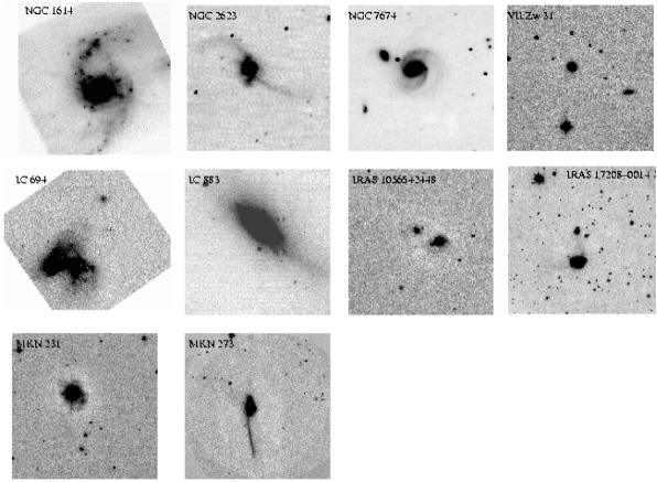
Figure 1.— The $H$-band images of the LIRG sample with a field of view of approximately 3$\arcmin\times 3\arcmin$, with north up and east to the left. The two HST/NICMOS images (NGC 1614 and IC 883) have fields of view of $\sim$ 30$\arcsec\times 30\arcsec$.

Figure 2.— One-dimensional spectra of the LIRG sample showing the CO absorption bandheads caused by the 2-0 and 3-1 molecular transitions. Mkn 231 was observed at 1.67 $\mu$m to measure the second overtone CO bands because of the dilution of the first overtone bands.

References

- (1)
- (2) Alonso-Herrero,, A., Rieke, G. H., Rieke, M. J., & Scoville, N. Z. 2000, ApJ, 532, 845
- (3)
- (4) Alonso-Herrero, A., Engelbracht, C. W., Rieke, M. J., Rieke, G. H., & Quillen, A. C. 2001, ApJ, 546, 952
- (5)
- (6) Barnes, J. E. & Hernquist, L. E. 1991, ApJ, 370, L65
- (7)
- (8) Barone, L. T., Heithausen, A., Hüttemeister, S., Fritz, T., & Klein, U. 2000, MNRAS, 317, 649
- (9)
- (10) Bryant, P. M. & Scoville, N. Z. 1999, AJ, 117, 2632
- (11)
- (12) Boselli, A., Lequeux, J., & Gavazzi, G. 2002, A&A, 384, 33
- (13)
- (14) Bushouse, H. A., et al. 2002, ApJS, 138, 1
- (15)
- (16) Charmandaris, V., et al. 2004, ApJS, 154, 142
- (17)
- (18) Colina, L., Arribas, S., & Monreal-Ibero, A. 2005, ApJ, 621, 725
- (19) Dasyra, K. M., et al. 2006, ApJ, 638, 745
- (20)
- (21) Djorgovski, S. & Davis, M. 1987, ApJ, 313, 59
- (22)
- (23) Downes, D. & Solomon, P. D. 1998, ApJ, 507, 615
- (24)
- (25) Dressler, A., Lynden-Bell, D., Burstein, D., Davies, R. L., Faber, S. M., Terlevich, R., & Wegner, G. 1987, ApJ, 313, 42
- (26)
- (27) Egami, E., et al. 2004, ApJS, 154, 130
- (28)
- (29) Engelbracht, C. W., Rieke, M. J., Rieke, G. H., Kelly, D. M., & Achertermann, J. M. 1998, ApJ, 505, 639
- (30)
- (31) Farrah, D., et al. 2001, MNRAS, 326, 1333
- (32)
- (33) Franx, M., Illingworth, G. & Heckman, T. 1989, ApJ, 344, 61
- (34)
- (35) Gallais, P., Charmandaris, V., Le Floc’h, E., Mirabel, I. F., Sauvage, M., Vigroux, L., & Laurent, O. 2004, A&A, 414, 845
- (36)
- (37) Genzel, R., Tacconi, L. J., Rigopoulou, D., Lutz, D., & Tecza, M. 2001, ApJ, 563, 527
- (38)
- (39) Hernquist, L. 1992, ApJ, 400, 460
- (40)
- (41) Hernquist, L. 1993, ApJ, 409, 548
- (42)
- (43) Hibbard, J. E., & Yun, M. S. 1999, AJ, 118, 162
- (44)
- (45) Israel, F. P. 1997, A&A, 328, 471
- (46)
- (47) Israel, F. 2000, Molecular hydrogen in space, Cambridge, UK: Cambridge University Press, 2001. xix, 326 p.. Cambridge contemporary astrophysics. Edited by F. Combes, and G. Pineau des Forêts. ISBN 0521782244, p.293, 293
- (48)
- (49) Kennicutt, R. C., Jr. 1998, ApJ, 498, 541
- (50)
- (51) Kim, D.-C., Sanders, D. B., Veilleux, S., Mazzarella, J. M., & Soifer, B. T. 1995, ApJS, 98, 129
- (52)
- (53) Kleinmann, S. G. & Hall, D. N. B. 1986, ApJS, 62, 501
- (54)
- (55) Le Floc’h, E., et al. 2004, ApJS, 154, 170
- (56)
- (57) Lisenfeld, U., Isaak, K. G., & Hills, R. 2000, MNRAS, 312, 433
- (58)
- (59) Maloney, P. & Black, J. H. 1988, ApJ, 325, 389
- (60)
- (61) McCarthy, D. W., Jr., Ge, J., Hinz, J. L., Finn, R. A., & de Jong, R. S. 2001, PASP, 113, 353
- (62)
- (63) Narayanan D., Groppi, C. E., Kulesa, C. A., & Walker, C. K. 2005, ApJ, 630, 269
- (64)
- (65) Puxley, P. J. & Brand, P. W. J. L. 1999, ApJ, 514, 675
- (66)
- (67) Rix, H.-W. & White, S. D. M. 1992, MNRAS, 254, 38
- (68)
- (69) Rix, H.-W. & Zaritsky, D. 1995, ApJ, 447, 82
- (70)
- (71) Sanders, D. B., Scoville, N. Z., & Soifer, B. T. 1991, ApJ, 370, 158
- (72)
- (73) Sanders, D. B., Soifer, B. T., Elias, J. H., Madore, B. F., Matthews, K., Neugebauer, G., & Scoville, N. Z. 1988, ApJ, 325, 74
- (74)
- (75) Sargent, W. L. W., Schechter, P. L., Boksenberg, A., & Shortridge, K. 1977, ApJ, 212, 326
- (76)
- (77) Schmidt, M. 1959, ApJ, 129, 243
- (78)
- (79) Schweizer, F. 1986, Science, 231, 193
- (80)
- (81) Scoville, N. Z. & Good, J. C. 1989, ApJ, 339, 149
- (82)
- (83) Scoville, N. Z., Sargent, A. I., Sanders, D. B., & Soifer, B. T. 1991, ApJ, 366, L5
- (84)
- (85) Scoville, N. Z., Sanders, D. B., Sargent, A. I., Soifer, B. T., & Tinney, C. G. 1989, ApJ, 345, L25
- (86)
- (87) Scoville, N. Z. et al. 2000, AJ, 119, 991
- (88)
- (89) Scoville, N. Z., Sanders, D. B., & Clemens, D. P. 1986, ApJ, 310, L77
- (90)
- (91) Shier, L. M. 1995, Ph.D. Thesis, University of Arizona
- (92)
- (93) Shier, L. M., Rieke, M. J., & Rieke, G. H. 1994, ApJ, 433, L9
- (94)
- (95) Shier, L. M., Rieke, M. J., & Rieke, G. H. 1996, ApJ, 470, 222
- (96)
- (97) Simkin, S. 1974, A&A, 31, 129
- (98)
- (99) Solomon, P. M., Downes, D., Radford, S. J. E., & Barrett, J. W. 1997, ApJ, 478, 144
- (100)
- (101) Strong, A. W., Moskalenko, I. V., Reimer, O., Digel, S., & Diehl, R. 2004, A&A, 422, L47
- (102)
- (103) Tacconi, L. J., Genzel, R., Lutz, D., Rigopoulou, D., Baker, A. J., Iserlohe, C., & Tecza, M. 2002, ApJ, 580, 73
- (104)
- (105) Taniguchi, Y. & Ohyama, Y. 1998, ApJ, 509, L89
- (106)
- (107) Taniguchi, Y., & Wada, K. 1996, ApJ, 469, 581
- (108)
- (109) Tonry, J. & Davis, M. 1979, AJ, 84, 1511
- (110)
- (111) Toomre, A. & Toomre, J. 1972, ApJ, 178, 623
- (112)
- (113) Tremaine, S., Richstone, D. O., Byun, Y., Dressler, A., Faber, S. M., Grillmair, C., Kormendy, J., & Lauer, T. R. 1994, AJ, 107, 634
- (114)
- (115) Veilleux, S., Kim, D.-C., & Sanders, D. B. 2002, ApJS, 143, 315
- (116)
- (117) Williams, D. M., Thompson, C. L., Rieke, G. H., & Montgomery, E. F. 1993, Proc. SPIE, 1946, 482
- (118)
- (119) Yamaoka, H., Kato, T., Filippenko, A. V., van Dyk, S. D., Yamamoto, M., Balam, D., Hornoch, K., & Plsek, M. 1998, IAU Circ. 6859, 1
- (120)