Information content in the halo-model dark-matter power spectrum

Abstract

Using the halo model, we investigate the cosmological Fisher information in the non-linear dark-matter power spectrum about the initial amplitude of linear power. We find that there is little information on ‘translinear’ scales (where the one- and two-halo terms are both significant) beyond what is on linear scales, but that additional information is present on small scales, where the one-halo term dominates. This behavior agrees with the surprising results that Rimes & Hamilton (2005, 2006) found using $N$-body simulations. We argue that the translinear plateau in cumulative information arises largely from fluctuations in the numbers of large haloes in a finite volume. This implies that more information could be extracted on non-linear scales if the masses of the largest haloes in a survey are known.

1 Introduction

Valuable cosmological information is encoded in the large-scale structure of the Universe. Rimes & Hamilton (2005; 2006, RH) have studied how much cosmological Fisher information is in the non-linear dark-matter power spectrum. As a start, they considered the information about the initial amplitude $A$ of linear power. RH measured this information from the covariance matrix of power spectra from $N$-body simulations. Meiksin & White (1999), Scoccimarro, Zaldarriaga & Hui (1999, SZH) and Cooray & Hu (2001, CH) have also explored this covariance matrix, without explicitly using the information concept. RH found that, as expected, information is preserved on large, linear scales, but the behavior is surprising on smaller scales. On translinear scales ($k\sim 0.2-0.8{\ }h^{-1}{\,}{\rm Mpc}$), the information is mostly degenerate with that in the linear regime, but there is significant extra information on smaller scales. This does not mean that surveys reaching only translinear scales are useless, but that translinear scales contribute little extra information about $A$ in a survey extending into the linear regime. Such clearly demarcated behavior in different regimes is suggestive of the halo model, in which the power spectrum consists of a term on linear scales and a term from virialized haloes.

2 Method

The Fisher information about a parameter $\alpha$ given a set of data is defined (e.g. Tegmark, Taylor & Heavens, 1997) as

$$I_{\alpha}\equiv-\left\langle\frac{\partial^{2}\ln\mathcal{L}(\alpha|{\rm data})}{\partial\alpha^{2}}\right\rangle,$$ (1)

where $\mathcal{L}$ is the likelihood function of $\alpha$ from the data.

We discuss the information in the (hereafter, implicitly non-linear dark-matter) power spectrum $P(k)$ about the logarithm of the initial amplitude $A$ of the linear power spectrum $P^{\rm lin}(k)$. In this paper, the word ‘information’ is implicitly about $A$, although this framework also allows other parameters to be investigated. The information in measurements $P(k_{i})$ and $P(k_{j})$ of the power spectrum is (RH)

$$I_{A}=-\left\langle\frac{\partial\ln P(k_{i})}{\partial\ln A}\frac{\partial^{2}\ln\mathcal{L}}{\partial\ln P(k_{i})\,\partial\ln P(k_{j})}\frac{\partial\ln P(k_{j})}{\partial\ln A}\right\rangle.$$ (2)

We approximate the expectation value of the middle term on the right side of this equation (i.e. the Fisher matrix) with the inverse of the covariance matrix, $[C^{-1}]_{ij}$. Here, $C_{ij}\equiv\left\langle\Delta P(k_{i})\Delta P(k_{j})\right\rangle$, where $\Delta P(k_{i})$ is a fluctuation of an estimate away from the mean in $P(k_{i})$. This approximation is good if the distribution of estimates of power about their mean is Gaussian, which RH showed to be sufficiently so in this case.

We follow the procedure of RH to measure $I_{A}$. We use uncorrelated band powers $B(k_{i})$ with a diagonal Fisher matrix. The band powers are decorrelated in such a way that they retain the same expectation values as $P(k_{i})$. Following RH, we use an upper-Cholesky decomposition, ensuring that the information up to a given $k_{\rm max}$ is affected only by data for $k\leq k_{\rm max}$. The cumulative information $I_{A}(\leq k)$ which we measure in terms of band powers is then

$$I_{A}(\leq k)=-\left\langle\sum_{k=0}^{k_{\rm max}}\frac{\partial\ln B(k)}{\partial\ln A}\frac{\partial^{2}\ln\mathcal{L}}{\partial\ln B(k)^{2}}\frac{\partial\ln B(k)}{\partial\ln A}\right\rangle.$$ (3)

2.1 Covariance matrix construction

The covariance of the power spectrum in a survey of volume $V$ is the sum of a Gaussian term, which depends on the square of the power spectrum itself, and a term involving the (hereafter, implicitly non-linear) trispectrum (SZH; Hamilton, Rimes & Scoccimarro, 2006);

$$C_{ij}=\frac{1}{V}\left[\frac{(2\pi)^{3}}{V_{s,i}}2P(k_{i})^{2}\delta_{ij}+T_{ij}\right],$$ (4)

where $V_{s,i}$ is the volume of shell $i$ in Fourier space (proportional to $k_{i}^{3}$ for logarithmically spaced bins), and $T_{ij}$ is the trispectrum averaged over shells $i$ and $j$;

$$T_{ij}\equiv\int_{s,i}\int_{s,j}T({\mn@boldsymbol{k}}_{i},-{\mn@boldsymbol{k}}_{i},{\mn@boldsymbol{k}}_{j},-{\mn@boldsymbol{k}}_{j})\frac{d^{3}{\mn@boldsymbol{k}}_{i}}{V_{s,i}}\frac{d^{3}{\mn@boldsymbol{k}}_{j}}{V_{s,j}}.$$ (5)

To obtain the power spectrum and trispectrum, we use the halo-model trispectrum formalism developed by CH, which we sketch here. In the halo model, the matter power spectrum is the sum of one- and two-halo terms.

$$P(k) = P^{\rm 1h}(k)+P^{\rm 2h}(k)$$ (6)

$$= M^{0}_{2}(k,k)+P^{\rm lin}(k)[M^{1}_{1}(k)]^{2},$$ (7)

where $M^{\beta}_{\mu}$ are integrals over the halo distribution;

$$M^{\beta}_{\mu}(k_{1},\ldots,k_{\mu}) \equiv \int\int\left(\frac{m}{\bar{\rho}}\right)^{\mu}b_{\beta}(m)n(m,c)$$ (8)

$$\times u(k_{1},m,c)\cdots u(k_{\mu},m,c)\,dc\,dm.$$

Here, $\bar{\rho}$ is the mean matter density, $m$ is the halo mass, $c$ is the halo concentration as in the NFW profile (Navarro, Frenk & White, 1996), $b_{\beta}(m)$ is the $\beta$-order halo bias (Mo, Jing & White, 1997; Scoccimarro et al., 2001), and $u(k,m,c)$ is the halo profile in Fourier space, normalized to unity at $k=0$. Like CH, we use a distribution in halo concentration since its effect can be large for higher-order correlations.

The halo-model trispectrum is the sum of one-, two-, three-, and four-halo terms (CH; Cooray, 2001, appendix). We quote those terms which seem to have a simple physical explanation (Sect. 3.1): the one-halo term,

$$T^{\rm 1h}({\mn@boldsymbol{k}}_{i},-{\mn@boldsymbol{k}}_{i},{\mn@boldsymbol{k}}_{j},-{\mn@boldsymbol{k}}_{i})=M^{0}_{4}(k_{i},k_{i},k_{j},k_{j})$$ (9)

(the arguments of $T$ terms will be implicit henceforth), and the component of the two-halo term which comes from taking three points in one halo and one point in the second,

$$T^{\rm 2h}_{31}=P^{\rm lin}(k_{i})M^{1}_{3}(k_{i},k_{j},k_{j})M^{1}_{1}(k_{i})+3{\rm\ perm}.$$ (10)

In implementing the halo-model trispectrum, we use the same cosmological parameters as RH: $(\Omega_{\rm M},\Omega_{\Lambda},f_{\rm b},h,\sigma_{8})=(0.29,0.71,0.16,0.71,0.97)$. The only halo-model parameter change from CH in our fiducial model is our use of the Sheth & Tormen (1999, ST), instead of the Press-Schechter (1974), mass function. We evaluate the trispectrum in the center of each bin, performing only an angular average. For the fiducial model, we tried decreasing the bin size by a factor of five, which barely affected the cumulative information.

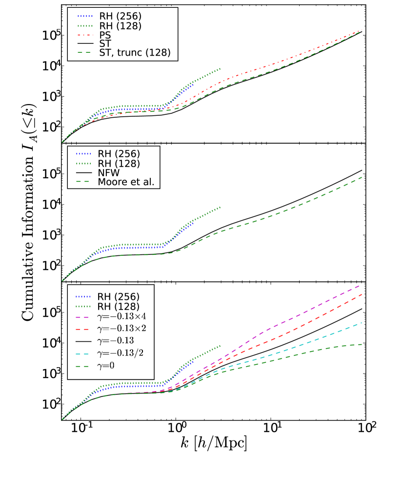
Figure 1: The Fisher information in the halo-model dark-matter power spectrum up to wavenumber $k$, as defined in Eq. 3, for different variants of the halo model. In each panel, the dotted curves show what RH found from hundreds of $N$-body simulations of box sizes 128 and 256${\ }h^{-1}{\,}{\rm Mpc}$. (For consistency, for the $128{\ }h^{-1}{\,}{\rm Mpc}$ box size, we use only the results of their 200 particle-mesh simulations.) Like RH, we normalize all $I_{A}(\leq k)$ for a $256{\ }h^{-1}{\,}{\rm Mpc}$ box. The solid black lines are from the fiducial model, with all halo-model inputs the same as in CH except for the mass function, which we take from Sheth & Tormen (1999); CH used a Press-Schechter (1974) mass function. The top panel shows that the mass function controls the shape of the translinear plateau. The dashed green curve is from an ST mass function calculated using $P^{\rm lin}(k<\frac{2\pi}{128{\ }h^{-1}{\,}{\rm Mpc}})=0$, truncated to mimic the conditions in a finite box. Changes in the small-scale slope of halo density profiles (middle panel) or in the slope $\gamma$ of the relationship between halo mass and concentration parameter (bottom panel) alter the small-scale shape of $I_{A}(\leq k)$. In the bottom panel, the curves rise as $\gamma$ grows more negative.

Using all the same parameters as CH, we obtained excellent agreement with the power spectrum they plotted. We also verified that our code gives the correct relevant $M^{\beta}_{\mu}$ functions in an analytical version of the halo model (Cooray & Sheth, 2002, $\S 4.3$). We used the convenient form of the angular-averaged perturbation-theory trispectrum provided by SZH (their eq. 7), and checked our perturbation-theory trispectrum against simple results they gave. Also, our $T^{\rm 1h}$ agrees with the covariance in $P^{\rm 1h}$ due to halo Poisson sampling, as theoretically expected (see appendix). However, our square-configuration trispectrum $\Delta^{2}_{\rm sq}(k)$ was slightly lower than that plotted by CH; also, our correlation matrix $\frac{C_{ij}}{\sqrt{C_{ii}C_{jj}}}$ appears to reach a given value at a slightly larger $k$ than in Table 1 of CH, by a factor of $\sim 1.5$. But these discrepancies are noticeable in the regime where the simple, well-tested $T^{\rm 1h}$ term dominates. After extensive tests, we are confident that our code is accurate. In any case, our qualitative result is insensitive to these slight differences.

3 Results

Figure 1 shows the cumulative information $I_{A}(\leq k)$ as found with the halo model under different sets of parameters, and as measured by RH from $N$-body simulations. All curves share these qualitative features: on linear scales, $I_{A}(\leq k)\propto k^{3}$, as expected; on translinear scales, there is little additional information; and on the smallest scales, the information rises again, but less steeply than in the linear regime. This small-scale rise seems to be shallower in the halo model than in simulations, although the small-scale measurements by RH were near their resolution limit.

Generally, the halo mass function affects the details of the translinear plateau in the cumulative information $I_{A}(\leq k)$, and halo density profiles affect the small-scale upturn. Changing the inner slope of the halo density profile between $-1$ (NFW) and $-1.5$ (Moore et al., 2001), fixing the density at the scale radius $r_{s}$, gives little change in $I_{A}(\leq k)$. We changed the slope $\gamma$ in the relation $c(m)=c_{0}(m/m_{\star})^{\gamma}$ between halo mass and concentration parameter more drastically; varying $\gamma$ from zero to four times its fiducial value, $-0.13$ (Bullock et al., 2001), has a large effect on $I_{A}(\leq k)$ on small scales. When $c(m)$ does not change with $m$, there is an apparent plateau in $I_{A}(\leq k)$ at the smallest scales, while $I_{A}(\leq k)$ is greatest when $c(m)$ falls off most sharply. Therefore, it could be said that the information on small scales is encoded in the systematic variation in halo density profiles with halo mass.

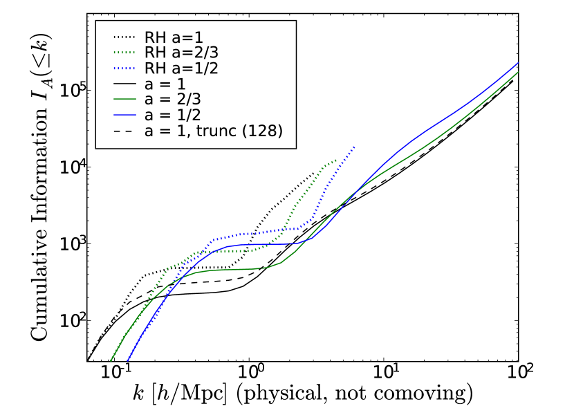
Figure 2: The information content of the halo-model power spectrum about the initial amplitude of the linear power spectrum, as a function of physical scale, for various redshifts. Also shown are the results from 200 particle-mesh simulations by RH, for boxes of size $128{\ }h^{-1}{\,}{\rm Mpc}$. For $a=1$, we also show the result if the linear power spectrum used for the ST mass function is truncated to mimic a box of this size. The information up to the physical scale of $100{\ }h{\,}{\rm Mpc}^{-1}$ in this fiducial model decreases slowly with time.

An interesting question which RH posed is whether the information (e.g., about $A$) in the power spectrum is preserved in time. If it is, then the cumulative information measured up to a fixed large physical (not comoving) wavenumber should remain constant in time. It would not make sense if information were created, but non-linear evolution could decrease with time; for example, it could divert into higher-order statistics. Requiring information to be preserved or lost is a test of the model which could be used to constrain halo-model parameters.

Our fiducial model passes this test; Figure 2 shows information curves as a function of physical $k$ for the fiducial model at fairly low redshifts (where the halo model is well-tested), along with curves from RH for comparison. Looking at the right edge of the figure, it seems that the halo model predicts that information up to a fixed physical scale of $100{\ }h{\,}{\rm Mpc}^{-1}$ gradually decreases with time.

3.1 Physical explanation: fluctuations in the number of large haloes in a finite volume

One reason to investigate the information concept with an analytic model is to gain physical insight. Much of the behavior of the cumulative information seems to come from the following Poisson halo abundance fluctuation (PHAF) effect: in a finite volume $V$, the number of haloes of mass between $m$ and $m+dm$ is not $Vn(m)dm$ (which would give fractional haloes), but is an integer drawn from a distribution with mean $Vn(m)dm$. We assume that the distribution is adequately Poissonian for haloes large enough that only a few may occur in the volume, and that the large number of smaller haloes is stable enough that non-Poissonianity in the distribution has a negligible effect.

In fact, the one-halo term $T^{\rm 1h}$ of the halo-model covariance corresponds to the covariance $\left\langle\Delta P^{\rm 1h}(k_{i})\Delta P^{\rm 1h}(k_{j})\right\rangle$ in $P^{\rm 1h}$ from Poisson-sampling the number of haloes in each bin. This can be shown analytically by considering mass bins small enough to contain only zero or one halo (see appendix). We also verified this numerically by comparing $T^{\rm 1h}$ to the covariance of $P^{\rm 1h}$ for 262144 Poisson realizations of the mass function. Compared to the true CH covariance in eq. (4), we consider the PHAF covariance to be an approximation which is not entirely accurate, but which shares two terms (see appendix) with the true covariance.

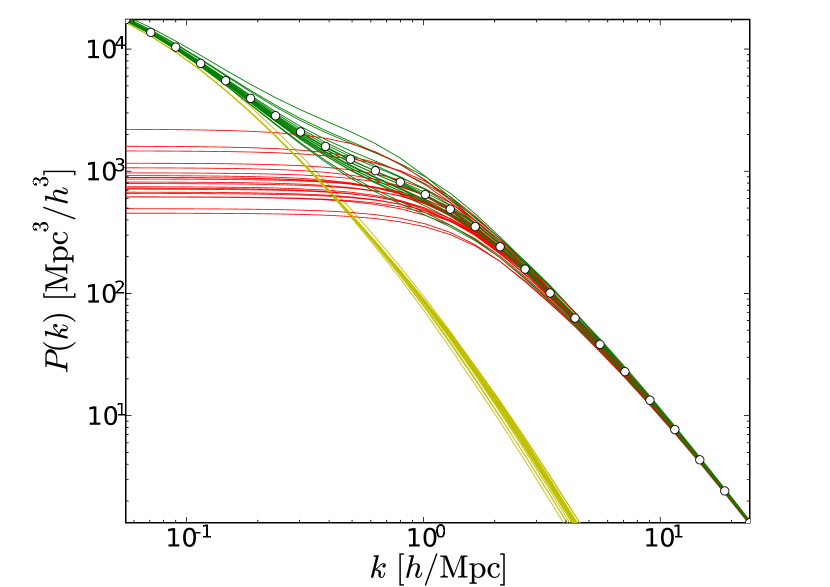
Figure 3: Power spectra from twenty realizations of an ST halo mass function for a volume $V=(128{\ }h^{-1}{\,}{\rm Mpc})^{3}$. The number of haloes in each mass bin $\delta(m)$ is drawn from a Poisson distribution of mean $Vn(m)\delta(m)$. The fluctuated 1- and 2-halo terms, and their sum, are shown in red, yellow, and green, respectively; the unfluctuated power spectrum appears as white dots. (The 2-halo terms are renormalized to agree with the linear power spectrum in the largest-scale bin.) There is a great deal of variance, and covariance, in the translinear regime, since it is here that Poisson fluctuations in the largest (rarest) haloes have the greatest influence on the power spectrum.

Figure 3 shows the power spectra from twenty Poisson realizations of the ST mass function in a volume $V=(128{\ }h^{-1}{\,}{\rm Mpc})^{3}$. (Fluctuating the mass function also causes $P^{\rm 2h}$ to fluctuate on large scales, but we have renormalized $P^{\rm 2h}$ to match $P^{\rm lin}$ in the largest-scale bin.) This pleisiosaur shape helps explain the shape of the information curve intuitively. Fluctuations in the number of the largest, rarest haloes in a finite volume lead to large variances (and covariances) in $P^{\rm 1h}$ on large scales. On translinear scales, this effect squelches the information. On larger, linear scales, information is preserved since $P^{\rm 2h}$ dominates, washing out the fluctuations in $P_{\rm 1h}$. On fully non-linear scales, the power spectrum is dominated by power from small haloes, which are more stable in their numbers, giving less covariance, and therefore significant information.

This pleisiosaur shape can also be understood as a dispersion in where $P(k)$ turns away from $P^{\rm lin}(k)$. This suggests that the HKLM ‘scaling Ansatz’ (Hamilton et al., 1991; Peacock & Dodds, 1996) may still be valid conceptually, despite RH’s apparent evidence to the contrary, if the dispersion in the function taking linear to non-linear power is properly taken into account.

Figure 4 shows how large a role $T^{\rm 1h}$ plays in the halo-model covariance. Keeping the Gaussian part from both terms of $P(k)$ fixed, but using only $T^{\rm 1h}$ for $T$, the information $I_{A}^{\rm 1h}(\leq k)$ shares some features with the full $I_{A}(\leq k)$. On small scales, $T^{\rm 1h}$ dominates $T$, and it is still significant on translinear scales. But this is not the whole story, since the translinear plateau of $I_{A}^{\rm 1h}(\leq k)$ is indistinct and wiggly. We have not determined the source of the wiggles, but odd behavior in $I_{A}^{\rm 1h}(\leq k)$ is not necessarily worrisome, since it uses only part of the physical $T$, yet uses the Gaussian covariance from the full $P(k)$.

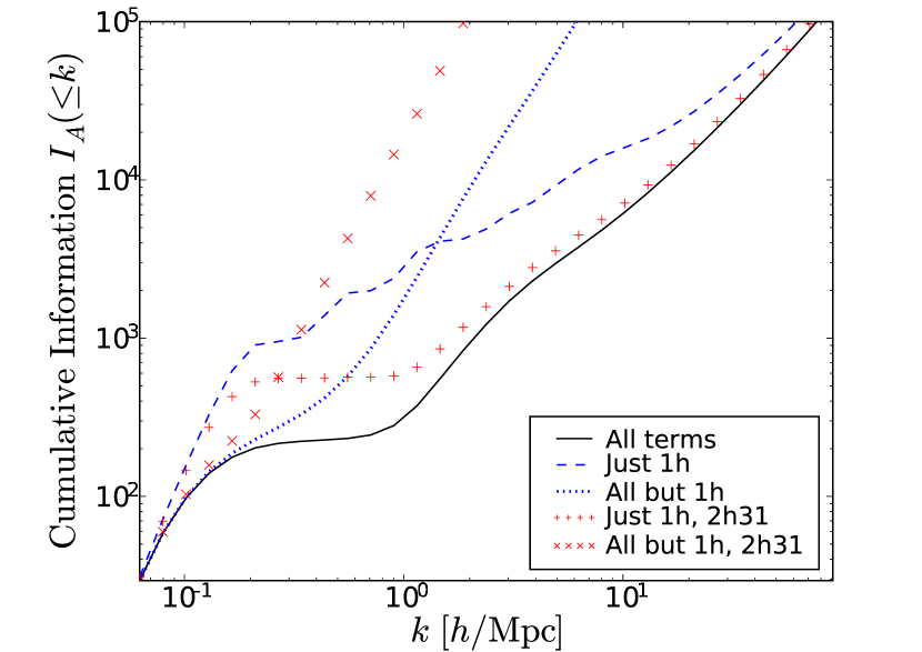
Figure 4: The information content in the halo-model power spectrum about the initial amplitude of linear power, if only $T^{\rm 1h}$, and $T^{\rm 2h}_{31}$ along with $T^{\rm 1h}$, are included in the trispectrum. Also shown is the information content if all halo-model trispectrum terms except these are included. The Gaussian piece of the covariance, using the full halo-model power spectrum, is always included. When covariance matrix terms are added, $I_{A}(\leq k)$ decreases, but not simply additively, since the Fisher matrix is a matrix inverse of a sum, not a sum of matrix inverses. The 1h term can be attributed to Poisson fluctuations in the halo mass function, as can, perhaps, $T^{\rm 2h}_{31}$. These two terms dominate the behavior of the information curve, indicating that Poisson halo fluctuations may largely be responsible for the loss of information in the non-linear regime.

There is also a term $\left\langle P^{\rm 1h}(k_{i})P^{\rm 2h}(k_{j})\right\rangle$ in the halo abundance fluctuation covariance (see appendix) which equals $T^{\rm 2h}_{31}$ (eq. 10). However, it is less certain that $T^{\rm 2h}_{31}$ may be attributed to PHAF. We measured the PHAF covariance of the full power spectrum, and found off-diagonal correlations near unity in the linear regime, which do not occur in linear theory. These high correlations come from $\left\langle P^{\rm 2h}(k_{i})P^{\rm 2h}(k_{j})\right\rangle$, in which mass function fluctuations cause $P^{\rm 2h}$ to be biased relative to $P^{\rm lin}$ by a constant (in $k$) on large scales. (This bias was removed in Fig. 3.) The error likely comes from replacing the bias $b_{2}(m)$ in the (true) CH covariance with $[b_{1}(k)]^{2}$ in the PHAF covariance. This replacement does not occur in $T^{\rm 2h}_{31}$, so we still attribute $T^{\rm 2h}_{31}$ to PHAF, but less confidently than we do $T^{\rm 1h}$. Figure 4 shows what happens if $T^{\rm 2h}_{31}$ is included or excluded along with $T^{\rm 1h}$; these two terms dominate the behavior of $I_{A}(\leq k)$.

4 Discussion

The qualitative agreement we found between power spectrum information content (about the initial amplitude $A$ of linear power) in the halo model and in $N$-body simulations (RH) is a success for the halo model paradigm describing the power spectrum and trispectrum. Our results also lend weight to the argument made by RH that the small-scale upturn in cumulative information, seen in their simulations, has a real, physical origin and is not the result of insufficient resolution. However, the agreement is not perfect, as with the bispectrum (Fosalba, Pan & Szapudi, 2005), so more halo-model ingredients, such as halo triaxiality (e.g. Smith, Watts & Sheth, 2006), may be necessary for the halo model to reach high precision for higher-order statistics. On the other hand, the high (co)variance on translinear scales suggests that inaccuracies in the halo model on these scales have less statistical significance than they seem.

Even if our information curves do not match exactly what RH found, the halo model allows us to understand their results better. The halo model will also allow the information about other cosmological parameters than $A$ to be studied easily. With a covariance matrix such as we used here, all that is needed to investigate another parameter $\alpha$ is $\frac{\partial P(k_{i})}{\partial\alpha}$, which the halo model can provide self-consistently.

Fluctuations in the number of haloes of a given mass (particularly, massive and rare ones) in a finite volume appear to be largely responsible for the paucity of cumulative information on translinear scales. Therefore, prospects for extracting cosmological information from the power spectrum on these scales might improve substantially with prior knowledge of the mass spectrum in a survey. For example, a conditional power spectrum depending on the mass of the largest cluster in a survey could contain significantly more information on non-linear scales than the power spectrum alone.

Appendix A Covariance from halo mass function fluctuations

Often in the halo model, integrals over halo mass functions are multiplied together. Formally, Poisson-sampling the halo mass function introduces an extra term in the expectation value of these products. Consider the ensemble average

$$\left\langle\int f(m)\tilde{n}(m)\,dm\int g(m)\tilde{n}(m)\,dm\right\rangle$$ (11)

over fluctuations $\tilde{n}(m)$ of the mean halo number density $n(m)$, where $f(m)$ and $g(m)$ are functions (e.g. halo density profiles) of mass. A Poisson realization of the mass spectrum may be considered, in a way reminiscent of Peebles’ (1980) derivation of power spectrum shot noise, by partitioning the mass function into bins $\delta(m_{i})$ small enough that in a given volume $V$, the number of haloes in each bin, $\phi_{i}\equiv V\tilde{n}(m_{i})\delta(m_{i})$, is 0 or 1. Expression (11) becomes

$$\frac{1}{V^{2}}\left\langle\sum_{i,j}f_{i}g_{j}\phi_{i}\phi_{j}\right\rangle=\frac{1}{V^{2}}\left\langle\sum_{i\not=j}f_{i}g_{j}\phi_{i}\phi_{j}\right\rangle$$

$$+\frac{1}{V^{2}}\left\langle\sum_{i}f_{i}g_{i}\phi_{i}\right\rangle,$$ (12)

since $\phi_{i}^{2}=\phi_{i}$. Returning to integral notation, this is

$$\int f\,n\,dm\int g\,n\,dm+\frac{1}{V}\int fg\,n\,dm.$$ (13)

Products of integrals over the mass function abound in the covariance $\left\langle\Delta P_{i}\Delta P_{j}\right\rangle$ of the halo-model power spectrum (eq. 7), where $\Delta P(k)=\tilde{P}(k)-P(k)$. Considering the product of two fluctuations in $P^{\rm 1h}$,

$$\left\langle\Delta P^{\rm 1h}(k_{i})\Delta P^{\rm 1h}(k_{j})\right\rangle=\frac{1}{V}M^{0}_{4}(k_{i},k_{i},k_{j},k_{j}),$$ (14)

which happens to be the one-halo term of the full CH covariance, eq. (9). Extending the notation of eq. (8) to allow more than one factor $b_{\beta}(m)$ in the integrand (e.g. $M^{11}_{2}(k,k)$ would have two $b_{1}(k)$ factors in the integrand), the 1h-2h term is, to order $1/V$ (there is also a $1/V^{2}$ term),

$$\left\langle\Delta P^{\rm 1h}(k_{i})\Delta P^{\rm 2h}(k_{j})\right\rangle= \frac{1}{V}P^{\rm lin}(k_{j})[M^{11}_{2}(k_{i},k_{i})M^{2}_{0}(k_{j},k_{j})+$$ (15)

$$2M^{1}_{1}(k_{i})M^{1}_{3}(k_{i},k_{j},k_{j})].$$

The second term here (when combined with the same term of $\left\langle\Delta P^{\rm 1h}(k_{j})\Delta P^{\rm 2h}(k_{i})\right\rangle$) is the CH covariance from $T^{\rm 2h}_{31}$; see eq. (10). To order $1/V$, the 2h-2h term is

$$\left\langle\Delta P^{\rm 2h}_{i}\Delta P^{\rm 2h}_{j}\right\rangle= \frac{P^{\rm lin}(k_{i})P^{\rm lin}(k_{j})}{V}[M^{11}_{2}(k_{1},k_{1})M^{1}_{1}(k_{2})^{2}+$$ (16)

$$2M^{11}_{2}(k_{1},k_{2})M^{1}_{1}(k_{1})M^{1}_{1}(k_{2})+$$

$$M^{11}_{2}(k_{2},k_{2})M^{1}_{1}(k_{2})^{2}].$$

If $M^{11}_{2}$ is replaced with $M^{2}_{2}$, the $M^{11}$ terms in eqs. (15) and (16) correspond roughly to $T^{\rm 2h}_{22}$ and the part of $T^{\rm 3h}$ which does not involve the bispectrum (see CH).

Taken at face value, eqs. (11, 13) have significant implications not only for the power spectrum covariance, but for the power spectrum itself, since the two-halo term involves the square of an integral over the mass function (eq. 7). By averaging together $P^{\rm 2h}$ from 262144 Poisson-sampled mass functions, we verified numerically that

$$\left\langle\tilde{M}^{1}_{1}(k)^{2}\right\rangle=M^{1}_{1}(k)^{2}+\frac{1}{V}M^{11}_{2}(k,k).$$ (17)

However, the $1/V$ halo discreteness term cannot contribute to the two-halo term. The two-halo term is the convolution of the halo-halo power spectrum with density profiles of two separate haloes, but in the halo discreteness calculation, there can only be (zero or) one halo in each bin, so the ‘$i=j$’ term does not contribute. A similar argument applies to terms in the halo-model trispectrum; the only terms which contain products of integrals over the mass function are multiple-halo terms. The covariance from halo discreteness, on the other hand, is meaningful because it involves a product of complete power spectrum terms.

References

- Bullock et al. (2001) Bullock J.S., Kolatt T.S., Sigad Y., Somerville R.S., Kravtsov A.V., Klypin A.A., Primack J.R., Dekel, A., 2001, MNRAS, 321, 559
- Cooray (2001) Cooray A., 2001, PhD thesis, Univ. Chicago
- Cooray & Hu (2001) Cooray A., Hu W., 2001, ApJ, 554, 56 (CH)
- Cooray & Sheth (2002) Cooray A., Sheth R., 2002, Phys. Rep., 372, 1
- Fosalba, Pan & Szapudi (2005) Fosalba P., Pan J., Szapudi I., 2005, ApJ, 632, 29
- Hamilton et al. (1991) Hamilton A.J.S., Kumar P., Lu E., Matthews A., 1991, ApJ, 374, L1
- Hamilton, Rimes & Scoccimarro (2006) Hamilton A.J.S., Rimes C.D., Scoccimarro R., 2006, MNRAS, submitted. (astro-ph/0511416)
- Meiksin & White (1999) Meiksin A., White M., 1999, MNRAS, 308, 1179
- Moore et al. (2001) Moore B., Quinn T., Governato F., Stadel J., Lake G., 1999, MNRAS, 294, 291
- Mo, Jing & White (1997) Mo, H.J., Jing, Y.P., White, S.D.M., 1997, MNRAS, 284, 189
- Navarro, Frenk & White (1996) Navarro J., Frenk C., White S.D.M., 1996, ApJ, 462, 563 (NFW)
- Peacock & Dodds (1996) Peacock J.A., Dodds S.J., 2000, MNRAS, 280, L19
- Peebles (1980) Peebles P.J.E., 1980, The Large Scale Structure of the Universe. Princeton Univ. Press, Princeton
- Press-Schechter (1974) Press W.H., Schechter P., 1974, ApJ, 187, 425 (PS)
- Rimes & Hamilton (2005) Rimes C.D., Hamilton A.J.S., 2005, MNRAS, 360, L82
- Rimes & Hamilton (2006) Rimes C.D., Hamilton A.J.S., 2006, MNRAS, submitted (astro-ph/0511518) (RH)
- Scoccimarro, Zaldarriaga & Hui (1999) Scoccimarro R., Zaldarriaga M., Hui L., 1999, ApJ, 527, 1 (SZH)
- Scoccimarro et al. (2001) Scoccimarro R., Sheth R., Hui L., Jain B., 2001, ApJ, 546, 20
- Sheth & Tormen (1999) Sheth R.K., Tormen G., 1999, MNRAS, 308, 119 (ST)
- Smith, Watts & Sheth (2006) Smith R.E., Watts P.I.R., Sheth R.K., 2006, MNRAS, 365, 214
- Tegmark, Taylor & Heavens (1997) Tegmark M., Taylor A.N., Heavens A.F., 1997, ApJ, 480, 22