Can Ejecta-Dominated Supernova Remnants be Typed from their X-ray Spectra? The Case of G337.2$-$0.7

Abstract

In this paper we use recent X-ray and radio observations of the ejecta-rich Galactic supernova remnant (SNR) G337.2$-$0.7 to determine properties of the supernova (SN) explosion that formed this source. H I absorption measurements from the Australia Telescope Compact Array (ATCA) constrain the distance to G337.2$-$0.7 to lie between $2.0\pm 0.5$ and $9.3\pm 0.3$ kpc. Combined with a clear radio image of the outer blast-wave, this distance allows us to estimate the dynamical age (between 750 and 3500 years) from the global X-ray spectrum obtained with the $XMM$-$Newton$ and Chandra observatories. The presence of ejecta is confirmed by the pattern of fitted relative abundances, which show Mg, Ar and Fe to be less enriched (compared to solar) than Si, S or Ca, and the ratio of Ca to Si to be 3.4$\pm$0.8 times the solar value (under the assumption of a single electron temperature and single ionization timescale). With the addition of a solar abundance component for emission from the blast-wave, these abundances (with the exception of Fe) resemble the ejecta of a Type Ia, rather than core-collapse, SN. Comparing directly to models of the ejecta and blast-wave X-ray emission calculated by evolving realistic SN Ia explosions to the remnant stage allows us to deduce that one-dimensional delayed detonation and pulsed delayed detonation models can indeed reproduce the major features of the global spectrum. In particular, stratification of the ejecta, with the Fe shocked most recently, is required to explain the lack of prominent Fe-K emission.

1. Introduction

A supernova (SN) explosion marks the death of a star, whether that be the gravitational collapse of a massive star that has run out of nuclear fuel at its core (core-collapse) or the disruption of a white dwarf by runaway nuclear reactions (Type Ia). The long-lived remnants of SN explosions provide a rich tapestry of information about the metal-rich ejecta produced in a SN, as well as the environment into which the remnant is expanding. X-ray spectra of supernova remnants (SNRs) are particularly useful given the extremely high shock temperatures and the fact that most cosmically abundant elements produced in the explosion have diagnostic K-shell lines in the 0.5 to 8.0 keV X-ray bandpass. Furthermore, the expansion of the ejecta allows their structure to be spatially resolved. Because X-ray emission from the ejecta can be identified thousands of years after the explosion, there exists a sample of young nearby SNRs despite a galactic SN explosion rate of only $\sim$1 per century. Given the diversity within the classes of core-collapse and Type Ia explosions, and the variety of open issues regarding their explosion mechanisms, it behooves us to study all the young SNRs in our Galaxy and nearby in the hope of gaining an understanding of the supernova explosions that originated them.

Evidence for metal-rich ejecta in SNR G337.2$-$0.7 was first found based on the strength of the emission lines in the ASCA X-ray spectrum (Rakowski et al. 2001). In that analysis, Si and S were confidently shown to be over-abundant compared to their solar abundances, and the pattern of metal abundances relative to each other was also highly non-solar. However the abundance ratios between the metals were not sufficiently well constrained to determine the origin of the SNR. In this paper, we analyze new observations of G337.2$-$0.7 with Chandra and $XMM$-$Newton$, and we complement these X-ray observations with radio data from the Australia Telescope Compact Array (ATCA). In our analysis, we devote special attention to the limitations of the techniques that are commonly used to measure elemental abundances, and how they influence our ultimate goal of determining the origin of this supernova remnant and contributing to our current understanding of SN explosions. Great care must be taken when interpreting X-ray spectra from SNRs because this emission will be dominated by the hottest, densest highly ionized material. Abundant elements can be hidden if they are in a low density low temperature region, not co-mingled with the bulk of the ejecta. Even amongst the bright ejecta, if the standard single electron temperature, single ionization timescale models are used, hot plasma may be misinterpreted as overabundances.

From the theoretical side, numerical simulations of SNe are rapidly increasing in sophistication. The inclusion of magnetic fields, angular momentum, asymmetries, and instabilities in the flow all require a 3-D treatment and are beginning to be explored in both core-collapse and Type Ia explosions. In this introduction we highlight some of the core issues under debate in the theory of SN explosions, which will set the context for our in-depth analysis of G337.2$-$0.7.

A key question for core-collapse explosions is what rejuvenates the shock after core-bounce. When the in-falling material forces the core of the star to such a high density that a neutron-rich nuclear composition is favored, the core stiffens and pushes back (“core-bounce”). However, in spherically symmetric simulations, this shock will stall against the force of the continually infalling material and fail to cause an explosion. A multi-dimensional mechanism is required to revitalize the shock, with the contenders including jet-induced explosions (Khokhlov et al., 1999; Wheeler et al., 2002; Maeda et al., 2002; Akiyama et al., 2003), neutrino driven convection (Fryer & Heger, 2000; Kifonidis et al., 2003; Kotake et al., 2003; Burrows et al., 2005), and turbulent dissipation of magneto-rotational energy (Thompson et al., 2005). Magneto-hydrodynamically (MHD) driven jets have particularly been proposed as a mechanism for gamma-ray burst (GRB) explosions (Wheeler et al., 2002; Maeda et al., 2002). The magnetic field may be pre-existing or it could be amplified by the magneto-rotational instability (Akiyama et al., 2003). There have also been improvements in neutrino transport calculations (Livne et al., 2004) and the incorporation of rotation into neutrino-driven convection models (Fryer & Heger, 2000; Kotake et al., 2003; Burrows et al., 2005). Including rotation naturally leads to a bi-polar structure in the neutrino flux and accretion of mass, such that the increased neutrino heating is sufficient and directed enough to revitalize the shock near the poles and explode the star. Alternatively, the rotational energy of the in-falling material itself can be converted into another source of heating behind the stalled shock by turbulent dissipation of the differential shear via the magneto-rotational instability (Thompson et al., 2005).

Simulations of white dwarf explosions are also progressing. The main difficulty is in constructing a realistic explosion that reproduces the abundances and stratification of the ejecta inferred from Type Ia spectra (e.g. Branch et al., 2005, and references therein). In one dimension, supersonic flame propagation (detonation) can burn almost the entire star to Fe-group elements because the star retains the original density ahead of the flame. A purely sub-sonic flame (deflagration) will push the star outwards, reducing the density of the material ahead of the shock. This causes the flame to be quenched earlier than in the detonation case and leave behind a large outer shell of unburnt material. Neither pure detonation nor pure deflagration produces the necessary quantities of intermediate mass elements (between O and Fe). The ad hoc solution in one dimensional simulations that successfully matches observation has been to invoke a transition from sub-sonic to supersonic flame propagation at some critical density, a “delayed detonation” (Khokhlov, 1991). Phenomenologically, this allows the star to expand first before the detonation front runs through it, thus creating a wider region of incomplete burning where Si, S, Ar, and Ca are produced before the flame is quenched. Considerable effort is going into simulating the actual turbulent burning front over a range of different scales to look for evidence of such a transition (Röpke et al., 2003; Röpke & Hillebrandt, 2004, 2005; Bell et al., 2004a, b). However, although the results of multidimensional physical effects and micro-physics of the flame can be worked into the one-dimensional models, the flame propagation is inherently three-dimensional. Current three dimensional simulations have generally refrained from artificially inducing a transition to supersonic burning, but these pure deflagrations still suffer from a deficit of intermediate mass products just as they did in one dimension. The other difficulty is that the three dimensional simulations are almost all well-mixed, unlike the stratification seen in Type Ia spectra (Kozma et al., 2005). Plewa et al. (2004) have produced preliminary models that retain a stratified elemental structure in three dimensions, by initiating the burning at a single, slightly off-center point and having the resulting hot bubble break out on the WD surface to trigger a ’gravitationally confined detonation’. However if the seeds for instabilities are present at the earliest times they will rapidly run away to thoroughly mix burnt and unburnt material (Röpke & Hillebrandt, 2005).

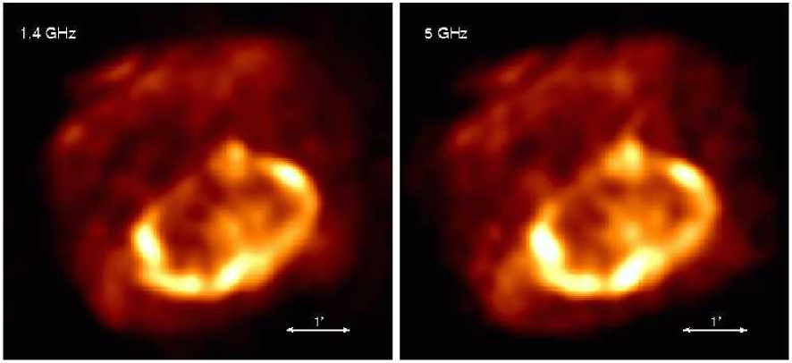
Figure 1.— ATCA 1.4GHz (left) and 5GHz (right) images of SNR G337.2$-$0.7 smoothed to 15″resolution (North:up East:left). The intensities are linearly scaled from 0 to 20 mJy per beam (1.4GHz) and 0 to 10 mJy per beam (5GHz).

The study of young SNRs is playing an increasingly important role in uncovering the SN explosion mechanism. For example, the “jet” in the northeast corner of Cassiopeia A (Cas A), first detected in the optical fast-moving S-rich knots by van den Bergh & Dodd (1970), has been cited as a possible example of the jet-induced core-collapse explosion model (Khokhlov et al., 1999). However, Hughes et al. (2000a) found that the composition of the X-ray emitting portions of the jet was more easily explained by Si-rich explosive Oxygen burning with little or no Fe, suggesting that the jet material originated further out in the exploding star. In contrast, to the southeast, Hughes et al. (2000a) found knots of almost pure Fe out past the bulk of the Si-rich ejecta. In deeper Chandra observations, Hwang & Laming (2003) confirmed the composition of these knots, finding others that could be explained by a pure Fe plasma. The high-velocity Fe-rich bullets in Cas A are reminiscent of the bullets of near-core material that would be ejected as a convection cycle broke through the stalled shock in the neutrino-driven explosion models of Burrows et al. (1995). This model was motivated by the early detection of Fe in the spectrum of SN 1987A. However, reproducing both features, Ne-rich bullets and a “jet” that originated further from the core, in one model is somewhat problematic (Burrows et al., 2005).

Type Ia SNRs have also shown interesting structures that lead to constraints on the explosion mechanism. Specifically, the stratification observed in Type Ia SN spectra is also seen in Type Ia SNRs. In the remnant of SN 1006 multiple lines of evidence point to stratification of the Si and Fe ejecta both from ultra-violet absorption lines of Si and Fe (e.g. Hamilton et al., 1997) and the lack of Fe-L emission in the X-rays (Vink et al., 2003). In Tycho’s SNR, spatially resolved spectroscopy of the ejecta supports the idea of stratification of conditions and composition (Vancura et al., 1995; Hwang & Gotthelf, 1997; Badenes et al., 2003). Detailed comparisons of Tycho to one and three dimensional Type Ia SN explosion models have shown that one-dimensional, stratified “delayed detonation” models best reproduce the spatial composition of Tycho’s SNR while recent well-mixed three-dimensional deflagration models fail (Badenes et al., 2005b).

These considerations regarding SN explosions are the context for our interpretation of the new $XMM$-$Newton$, Chandra and ATCA X-ray and radio observations of G337.2$-$0.7, an ejecta-rich remnant that still bears a clear imprint from the explosion that produced it. In Section 2 we outline the radio and X-ray observations and data reduction. The radio and X-ray morphologies of G337.2$-$0.7 are compared in Section 3 and an estimate of the distance to the remnant is found from H I absorption measurements in Section 4. Section 5 discusses the results of non-equilibrium ionization (NEI) modeling of the global X-ray spectrum of the remnant. The validity of utilizing a single temperature model for the global spectrum is investigated with respect to spatial variations throughout the remnant in Section 6. We then proceed to compare the results of our global NEI model to the predicted abundances from core-collapse and Type Ia SN models in Section 7. A detailed comparison of the global spectrum to the Type Ia model SNR spectra from Badenes et al. (2003) is performed in Section 7.1. We conclude by incorporating the results of these various investigations into a single picture of the ejecta-rich SNR G337.2$-$0.7 (Section 8).

2. Data, Processing, and Calibration

2.1. Radio Observations

We have obtained radio observations of G337.2$-$0.7 at multiple frequencies using the ATCA, a six-element aperture synthesis telescope located near Narrabri, Australia (Frater et al., 1992). Observations centered at frequencies of 4672, 4800 and 5312 MHz were carried out on 1999 July 19/20 in the 0.75D configuration, using a bandwidth of 128 MHz at each frequency and for a total effective integration time of 6.5 hours. Subsequent observations were carried out on 2004 Jul 13 (in the 6A configuration) and 2004 Dec 18 (in the 1.5D configuration), each recording data simultaneously at 1384 MHz (using a 128 MHz bandwidth) and in the H I line (using a 4 MHz bandwidth) for a total integration time of 20.5 hours. To recover the full range of spatial scales in the H I line, we also made use of shorter interferometer spacings from the Southern Galactic Plane Survey (SGPS) (McClure-Griffiths et al., 2005).

The ATCA data were edited and calibrated using standard techniques. Observations at 4672, 4800 and 5312 MHz were then combined into a single image (hereafter referred to as the 5-GHz image), while the 1384 MHz data were imaged separately (hereafter referred to as the 1.4-GHz image). Both images were deconvolved using maximum entropy, smoothed with a Gaussian restoring beam, and then corrected for primary beam attenuation. Residual atmospheric gain variations were significant for the 5 GHz data; these were corrected using two iterations of phase self-calibration.

The final 1.4-GHz image has a resolution of $8^{\prime\prime}\times 6^{\prime\prime}$ and a sensitivity of 70 $\mu$Jy beam^-1, while the 5-GHz image has a resolution of $12^{\prime\prime}\times 10^{\prime\prime}$ and a sensitivity of 90 $\mu$Jy beam^-1. The resulting maps are shown in Figure 1, and in both cases are expected to be sensitive to all spatial scales associated with the SNR. The corresponding flux densities of the SNR are $1.55\pm 0.05$ Jy at 1.4 GHz and $0.93\pm 0.02$ Jy at 5 GHz, in both cases using observations of PKS B1934–638 referenced to the scale of Reynolds (1994). This implies a spectral index $\alpha=-0.4$ ($S_{\nu}\propto\nu^{\alpha}$), which is well within the typical range for SNRs.

For the H I observation, continuum emission was subtracted from the data in the visibility plane. The data were then imaged at a velocity resolution of 3.3 km s^-1, using a spatial filter aimed at excluding H I emission on larger scales while retaining sensitivity to absorption on spatial scales corresponding to structure in the SNR. The emission cube was then deconvolved using the CLEAN algorithm, and restored to a resolution of $39^{\prime\prime}\times 36^{\prime\prime}$.

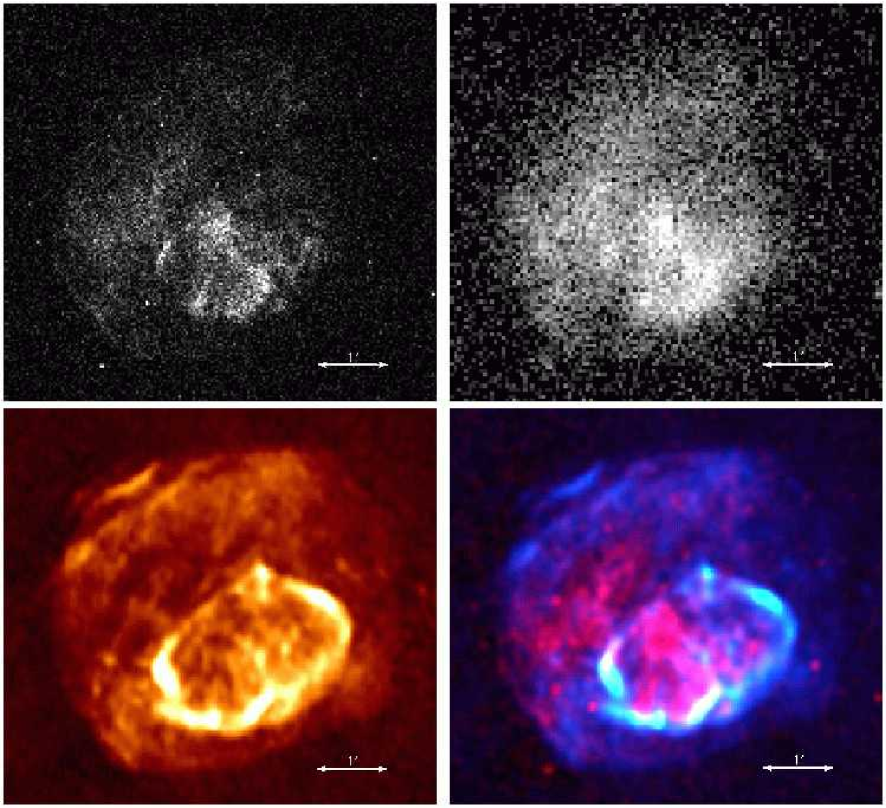
Figure 2.— X-ray and radio images of SNR G337.2$-$0.7. Upper left: broadband 1 to 5 keV Chandra image, binned by four pixels, linearly scaled from 1 to 12 counts per bin. Upper right: combined $XMM$-$Newton$ MOS1 and MOS2 image of G337.2$-$0.7 from 1 to 5 keV. Square-root scaling was chosen in this image to emphasize the fainter diffuse emission, almost filling the extent of the radio remnant. Lower left: Full resolution 1.4 GHz ATCA image linearly scaled from 0 to 4 mJy per beam. Lower right: Overlay of the broadband Chandra X-ray (red) and the 1.4 GHz ATCA radio (blue-green) images. An arbitrary scaling was chosen to show both faint (blue) and bright (green) radio emission against a smoothed Chandra X-ray image (Gaussian kernel width 3 four-pixel bins) shown in red.

2.2. $XMM$-$Newton$ and Chandra X-ray Observations

G337.2$-$0.7 was observed for 38.4 ks by $XMM$-$Newton$  on 2001 Feb 18, observation ID 0087940101. Standard reduction and processing of the three EPIC datasets were carried out using available XMM-SAS 6.0.0 software. Starting from the level 1 event files, the latest calibrations were applied with the “emchain” and “epchain” tasks. The events were then filtered to retain only the “patterns” and photon energies likely for X-ray events: patterns 0 to 4 (single and double pixel events) and energies 0.2 to 15.0 keV for the PN, patterns 0 to 12 (including triple and quadruple events) and energies 0.2 to 12.0 keV for the two MOS instruments. Events near hot pixels, outside the field of view or otherwise suspect are “flagged” within the event file and were eliminated using the most conservative screening. Within the good time intervals, no significant flares were detected, and the background count-rate was consistent with that measured in average quiescent times. The effect of any undetected soft flares was minimized by the use of local background from the same observation that was extracted from an ellipsoidal annulus outside the supernova remnant. Spectra extracted from the PN, MOS1 and MOS2 cameras were fitted simultaneously to maximize statistical significance (after consistency between instruments was verified). Detector response files and effective areas for the extracted spectra were also generated with the standard XMM-SAS 6.0.0 software.

Chandra observed G337.2$-$0.7  for 48.8 ks with the back-side illuminated CCD ACIS S-3, beginning on 20 August 2002, observation ID 2763. These data were reprocessed using CIAO 3.1 and caldb 2.26. The events were first calibrated with the appropriate instrument response files using “acis_process_events,” then filtered on grade, on energy, and to eliminate bad pixels and periods of high background. The time-dependent gain correction was applied using the contributed software “TGAIN” from Alexei Vikhlinin (this is the same correction that is now available as part of “acis_process_events” in CIAO 3.2). All spectra were extracted with their own weighted response files using the “acisspec” task. Background contamination, primarily from the Galactic Plane region, was important for G337.2$-$0.7. For simplicity, an annulus around the SNR was used to subtract local background directly from each spectra (weighted by the ratio of the areas of the background and source regions). Images of G337.2$-$0.7 from $XMM$-$Newton$ and Chandra are shown in Figures 2 and 5.

3. Radio and X-ray Morphology

The 1.4 GHz and 5 GHz images of G337.2$-$0.7 are very similar when convolved to the same spatial scale (Figure 1). Both show faint diffuse emission from a 4.5′ $\times$ 5.5′ (diameter) SNR. A wider radio image of the Galactic plane (Green et al., 1999) shows G337.2$-$0.7 to be in an isolated region off the plane. While not a diagnostic of the progenitor type, one would expect a larger number of SNRs generated by Type Ia SNe than by core collapse SNe in this region, because Type Ia progenitor systems have more time to drift away from their birthplaces at low latitudes before the explosion than more massive stars do. The sharp edges that presumably demarcate the outer blast-wave appear to be somewhat squared off and only limb-brightened in a few regions. It is important to note that this is a genuine feature rather than an artifact due to the use of “clean boxes” — i.e., while the deconvolution process was constrained by the use of region selection, in both cases the boundaries of the regions used lay well outside the sharp edges seen here.

The most prominent feature at both radio frequencies is a bright elliptical ring 2.0′ $\times$ 3.2′ in extent in the south part of the SNR. Such a brightening in the radio must indicate an enhancement in the magnetic field, electron density or both. The ring is incomplete and clumpy, appearing primarily as short bright arcs with one spoke into the center and a bright clump in the north that extends outside the main ellipse. However, with the possible exception of the bright northern clump that may have a slightly flatter spectral index ($\sim-0.25$), the ring does appear to be a coherent structure with a constant spectral index, $-0.5\pm 0.1$ and weak linear polarization at 5 GHz (up to peaks of 10% fractional polarization at the ends of the major-axis).

The Chandra and $XMM$-$Newton$ (MOS1$+$MOS2) images are shown in the top panel of Figure 2. The higher resolution Chandra image has been scaled linearly to emphasize the bright clumps of X-ray emission near the radio ring, while the deeper $XMM$-$Newton$ image is square-root-scaled to show the faint diffuse emission that extends throughout most of the radio shell. The bottom panel of Figure 2 shows the 1.4 GHz image at full resolution on the left and a 3-color overlay of the Chandra X-ray (red) and ATCA 1.4 GHz (blue$+$green) images on the right. In this overlay, the fainter radio emission is shown in blue while the bright radio ring has been emphasized by displaying it in green (turquoise). Purple and white regions indicate an overlap between the X-ray emission and the faint or bright radio emission, respectively.

Looking outside of the bright radio ring, a wide band of X-ray emission north-east of the ring lies where the radio emission is weakest. A faint radio filament traces the brightest portion of this swath of X-ray emission (compare the 1.4 GHz image with the 3-color overlay). Elsewhere some amount of faint X-ray emission accompanies most of the faint radio emission inside the rim, with the possible exceptions of the narrow region south of the bright ring and the western-most side of the remnant. Along the limb-brightened portions of the radio rim, there are suggestions of X-ray emission above the background with one clear identification of an X-ray filament aligned with the radio rim in the south-east. This filament is brightest in the X-rays where it is faint in the radio, but they are clearly related since they share the same small indentation (located at the brightest part of the X-ray emission of the filament).

As for the bright ring itself, there is one short arc of X-ray bright material aligned with the northeastern tip of the radio ellipse, beginning just as the radio surface brightness is dropping. In the southern portion of the ring, the arcs of bright radio emission extend further out than their X-ray counterparts, while in the north-west no X-ray emission is seen from the strong radio arcs. The radio clump in the north of the ring shows only faint X-ray emission. Vice-versa the X-ray bright clump on the north-eastern side aligns with a particularly faint spot in the 1.4 GHz image, and the spoke of X-ray emission across the minor axis of the ellipse does not align well with the radio protrusion from the south rim.

The meaning of the differences and correspondences between the X-ray and radio morphologies is not obvious, but clearly deserves more attention. What insights into the origin of the bright radio ring could the X-ray spectral observations divulge? If the ring demarcates the current position of the reverse shock, that would imply higher abundances in the X-ray spectrum from that region. An interaction with some structure in the circumstellar or interstellar medium (ISM) should be reflected in lower abundances of high-Z elements. Some feature intrinsic to the explosion itself would be likely to have different abundance ratios of heavy elements than elsewhere. We address these issues further in Sections 6 and 7.1.

Figure 3.— H I absorption spectra from three regions in the field, G337.1$-$0.2 an unresolved H II region $\sim$11 kpc distant, the supernova remnant itself, and a blank-sky position about 2′ southwest at RA 16:39:14.151, Dec -47:53:43.52 (J2000). All absorption features to the H II region are point-like and hence real. Only the $-22$km s^-1 feature in the remnant spectrum distinctly followed the morphology of the SNR. Absorption near $-113$km s^-1 extended in a wide swath a few arcminutes in size. The bottom panel shows a sample spectrum from a source free region 2′ southwest of the remnant exhibiting clear absorption at $-110$km s^-1. Fractional absorptions relative to the 1.4 GHz continuum are plotted. Note that for the SNR these exceed an absolute value of 1 indicating the presence of H I self-absorption over this region, such as might be expected from the large molecular cloud seen in ¹²CO.

4. Constraints on the Distance to SNR G337.2$-$0.7

To constrain the distance to SNR G337.2$-$0.7 via H I absorption, we examined both the ATCA H I cube centered on G337.2$-$0.7, plus SGPS H I data on surrounding fields, both on a channel-by-channel basis. Real absorption features to G337.2$-$0.7 should be significantly deep and conform to the shape of the remnant. Figure 3 plots the fractional absorption for three targets in the field, G337.1$-$0.2 (an unresolved bright H II region $\sim 30^{\prime}$ northwest of the SNR, at a distance of 11 kpc Corbel et al. (1999)), the supernova remnant itself and a blank-sky position about 2′ southwest of the remnant. The strongest absorption features toward G337.1$-$0.2 are at Local Standard of Rest (LSR) velocities of $-$22 km s^-1 and $-$116 km s^-1 (see also Fig. 4 of Sarma et al., 1997). The channel images show both to be entirely point-like and thus truly along the line of sight to this unresolved H II region. SNR G337.2$-$0.7 shows absorption at $-$22 km s^-1 which conforms to the shape of the remnant, but the next strongest absorption feature at $\sim-$116 km s^-1 extends evenly across a wide swath of the image as can be seen in the blank-sky spectrum in the bottom panel of Figure 3. Given that the ¹²CO survey of Dame et al. (2001) shows that cold absorbing gas at this velocity covers the sight-lines toward both G337.2$-$0.7 and G337.1$-$0.2 we take the lack of absorption specific to the SNR at $-$116 km s^-1 to be significant and to indicate that the SNR is closer than this cloud.

We thus adopt $-$22 km s^-1 and $-$116 km s^-1 as upper and lower limits, respectively, on the systemic velocity of G337.2$-$0.7. Using the Galactic rotation curve of Fich et al. (1989), and assuming a distance to the Galactic Center of 8.5 kpc, we constrain the distance to G337.2$-$0.7 to be between $2.0\pm 0.5$ kpc and $9.3\pm 0.3$ kpc, where we have assumed typical uncertainties of $\pm 7$ km s^-1 in the velocity of each H I feature. In the final analysis we also consider the possibility that general absorption in the region around G337.2$-$0.7 has obscured a true absorption feature at $-116$km s^-1 , i.e. that we should ignore the upper limit on the distance.

5. X-ray Spectral Analysis: The Global Spectrum of the Remnant

5.1. An Aside on the Usage of the Word Abundance

Given that the primary subject of this paper is to reconcile the abundance pattern that we see in the spectra of SNR G337.2$-$0.7 with its radio and X-ray morphology, as well as directly with SN explosion model predictions, it is worthwhile to first clarify exactly to what we are referring. When speaking of the abundances there are many things to consider. The first distinction to make is between “fitted abundances,” i.e. how much of any given element is inferred from a spectrum, and the overall metal production predicted by a SN model. The fitted abundances generally assume a single electron temperature and timescale and are actually proportional to the “volume emission measure” (EM) which is the product of electron density times the ion density integrated over the emitting the volume. Not only might some of the ejecta be at lower temperatures than others but if the density in a particular layer is too low it simply will not be seen. For example, in the Type Ia SNR models of Badenes et al. (2003) there are cases where the relative emission measures of elements compared to relative masses produced can be different by 3 or 4 orders of magnitude. In fact, the less abundant element can appear to be the more abundant one (see O versus Fe in Figure 4b of Badenes et al., 2003). Under these circumstances, it is clear that comparing globally fitted abundances to the bulk chemical composition obtained from a SN explosion model is not always justified, and can lead to erroneous conclusions. The second hurdle is the notation used for fitted abundances. Conventionally in NEI modeling, especially in XSPEC, the “abundance” of an element is defined by a linear factor relative to its “solar abundance.” The solar abundance set is written on the logarithmic “dex” scale for the number of atoms ($n_{X}$) of each element ($X$) relative to the number of hydrogen atoms ($n_{\rm H}$) as follows: $dex(X)=12.0+log(n_{X}/n_{\rm H})$. In contrast, SN modelers generally report the solar masses of each element produced, not the number. Once the presence of ejecta in the emitting region has been detected by the fitted abundances, it is often the case that the abundances of the metals relative to each other are better constrained than the number of atoms relative to hydrogen. Thus, throughout this paper we will refer to both the “abundance” of any given element (relative to hydrogen relative to solar) and the “relative abundances” or “abundance ratios” of one metal to another. These relative abundances will be given with respect to their solar ratio. For example, a Ca to Si ratio of 2 times solar, does not imply that there are twice as many Ca atoms as Si atoms but rather that there are twice as many Ca atoms per Si atom as would be present in a “solar abundance plasma.” Further, we will refer to the set of metal abundance ratios as the “abundance pattern” (listed relative to Si). Normalizing elemental abundances to a given “solar” composition is useful for studies of the ISM, but it is often an awkward convention for SN ejecta, especially in the case of Type Ia SNe, which have no H in the ejecta.

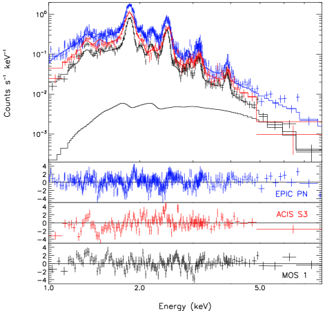
Figure 4.— $XMM$-$Newton$ EPIC PN, MOS 1 and Chandra ACIS S-3 spectra of the overall SNR G337.2$-$0.7. (The MOS 2 spectrum is similar to MOS 1). The model is a non-equilibrium ionization thermal plasma model with the abundances of Ne, Mg, Si, S, Ar, Ca and Fe allowed to vary along with the absorbing column density, the ionization timescale and the electron temperature. An additional power-law component significantly improved the fit. An example of the contribution of the second component to the overall model is plotted here for MOS1. The spectra have been re-binned to signal-to-noise of 4 for plotting purposes only.

5.2. NEI Model Fitting Procedure

The global SNR spectrum contained 13900, 14500, 23900 and 34200 counts from MOS1, MOS2, PN, and ACIS-S3 respectively. To begin, the spectrum from each instrument was fit independently with a planar shock NEI model. The shock model used is described in Hughes et al. (2000b) and allows a variable electron temperature, $kT_{\rm e}$, final ionization timescale, $n_{\rm e}t$, and normalization. This model includes lines from Mewe et al. (1985) that are important during the transient ionizing stage as described in Hughes & Singh (1994). Planar shock models are widely used as a first approximation to the spectrum of a complex SNR in order to obtain estimates of the bulk properties and abundances of the ejecta (or blast-wave) by initially assuming that all emitting material is under the same conditions. During the fitting procedure, the abundances of all elements were initially held at their solar ratios, but freed as necessary where the data could clearly constrain the individual abundances. The NEI model was convolved with an absorption model (using solar abundances) for the interstellar column density, $N_{\rm H}$. Where the statistics warranted it, a power-law component was also included to account for additional high-energy continuum emission that could be coming from either non-thermal X-ray synchrotron emission (appropriate for the power-law model used here) or a second, higher temperature thermal component (explored further in Sections 7 and 7.1). Although small shifts in the line centroids between instruments could be seen (of order 15 keV, similar to those found in $XMM$-$Newton$ analysis of Kelper’s SNR Cassam-Chenaï et al., 2004) no significant differences in the fits between instruments were found for spectra extracted from any region. All small differences in the fitted parameters could be explained by the different quantum efficiencies for the PN, the MOS, and ACIS-S3 which effected what portion of the spectrum had the greatest statistical weight.

The PN, MOS1, MOS2 and ACIS-S3 spectra of the overall SNR were then fitted simultaneously with a single NEI model. The only parameter that was allowed to differ between the instruments was the normalization which varied slightly, most probably owing to imperfect area calculations around the chip gaps, hot and dead pixels. An iterative process of fitting each of the instruments individually and then in combination was used for speed to locate the area of parameter space where the best fit would lie. This was followed by a thorough search of the surrounding area of parameter space using all four instruments to identify the best-fit and constrain the 1$\sigma$ uncertainty ranges of all the parameters. The results of these fits are given in Table 1.

Table 1NEI Parameters for the Global Spectra of SNR G337.2$-$0.7

	ASCA	$XMM$-$Newton$ & Chandra
$N_{\rm H}$ ($10^{22}$ cm-2)	$3.5\pm 0.3$	$3.2\pm 0.1$
$kT_{\rm e}$ (keV)	$0.85^{+0.04}_{-0.03}$	$0.74^{+0.03}_{-0.01}$
log($n_{\rm e}t$) log(cm-3s)	$12.25^{+\inf}_{-0.43}$	$12.02^{+0.05}_{-0.08}$
$n_{\rm e}n_{\rm H}V/4\pi D^{2}$ cm-5	$1.7\times 10^{12}$	$(2.0\pm 0.4)\times 10^{12}$
Ne	$0.0^{+2.1}$	$4.16^{+0.84}_{-1.64}$
Mg	$0.0^{+2.1}$	$1.74^{+0.20}_{-0.40}$
Si	$5.4^{+12.2}_{-2.2}$	$3.50^{+0.24}_{-0.62}$
S	$4.7^{+9.9}_{-1.8}$	$5.04^{+0.32}_{-0.82}$
Ar	$2.7^{+4.6}_{-1.1}$	$1.69^{+0.11}_{-0.26}$
Ca	$2.8^{+7.1}_{-2.8}$	$11.77^{+0.83}_{-2.04}$
Fe	$6^{+19}_{-3}$	$0.98^{+0.18}_{-0.29}$
Ni		$0.0^{+0.126}$
$\Gamma$		$2.2^{+0.2}_{-0.5}$
photons cm-2 keV-1 s-1		$(4.0\pm 2.5)\times 10^{-4}$
$\chi$ (dof)	103.1(67)	2023(1348)
$\chi_{r}^{2}$	1.539	1.501

5.3. Results from the Global SNR Spectrum

First let us consider how the overall SNR spectrum compares with our previous ASCA  results and conclusions about the remnant’s dynamical state (Rakowski et al., 2001). The overall best-fit column density, electron temperature, ionization timescale and normalization derived from the ASCA spectrum are all reasonably consistent with the more well-constrained $XMM$-$Newton$ and Chandra  results. The main result from the ASCA  spectrum was the presence of a significant amount of ejecta as exhibited by the prominent Si, S and Ar lines. The overabundance of these three species is clearly demonstrated in the new observations, with a better and more tightly constrained fit to their ionization state, allowing us to more precisely determine their abundances. Furthermore, a strong Ca component, which was hinted at with one outlying point above the ASCA  model, is firmly detected with the far superior effective area of $XMM$-$Newton$ and Chandra. The only difference between the ASCA and the $XMM$-$Newton$ and Chandra best-fit abundances lies in the prediction for Ne, Mg and Fe. The ASCA  results for these species were based solely on the 1-2 keV portion of the spectrum, where Ne and Mg K$\alpha$ lines and Fe-L lines should lie. However, no strong evidence for particular lines was seen, and the model preferred to fill in that region with Fe-L emission. The $XMM$-$Newton$  and Chandra spectra, however, exhibit a prominent Mg line and should be sensitive enough to reveal an Fe-K line (at $\sim$6.7 keV), under the assumptions of a single temperature planar model, if Fe were truly super-solar in abundance. Hence the deeper $XMM$-$Newton$ and Chandra spectra prefer the combination of a less-absorbed, cooler continuum plus Ne and Mg lines rather than a more highly absorbed continuum and Fe-L lines to fit the soft emission. However, even this best-fit model only approximates, but does not reproduce, the features around the He-like Mg K-shell “triplet” at $\sim$1.34 keV. For any single instrument, discrepancies from the model of similar magnitude occur across the entire spectrum (see the residuals in Figure 4). However, for the most part the residuals from different instruments do not all agree in sign or trend, whereas around 1.5 keV and below all three exhibit a similar pattern (the MOS 2 spectrum is similar to that of MOS 1). Combined with the fact that there are two alternative minima in $\chi^{2}$ to explain the soft emission, it is fair to say that the Ne, Mg and Fe results are less conclusive than for Si, S, Ar and Ca.

The new X-ray observations strongly indicate the presence of an additional spectral component. The greater than 150 reduction in $\chi^{2}$ for the addition of a powerlaw is highly significant (F-statistic probability of chance occurence: 5.6$\times 10^{-20}$). Unfortunately the nature of the second component is not constrained by these spectra. An additional thermal component results in an equally viable fit (see Section 7). For the purposes of this section the question is how has the addition of a powerlaw component changed the fitted abundance pattern from the $XMM$-$Newton$ and Chandra spectra. As would be expected, the abundances increase systematically when a second component is allowed to explain part of the continuum emission. However the relative abundances of Si,S, and Ar are virtually unchanged and [Ca/Si] is increased but only from 3.09 to 3.4 [Ca/Si]_☉. Without a second component, the Ne and Mg abundances relative to Si drop below solar, but their presence is still required for the fit. The Fe abundance in the single component fit drops steeply partially because a higher electron temperature (1.1 versus 0.74 keV) is required to explain the high energy continuum.

Given our new X-ray parameters along with the more well-defined size and distance from the radio observations we can refine our previous estimates of the ambient density and age of the remnant to see if these are consistent with a young ejecta-dominated SNR. For a first estimate, we assume that the normalization and temperature of our single temperature fits are dominated by the blast-wave component so that we can compare them to an analytical Sedov solution for the expansion of a middle-aged SNR into a uniform density medium. Following Hughes et al. (1998), we obtain the following values for the ambient density, $n_{\rm H}$, age, explosion energy, $E_{0}$, and amount of swept-up interstellar material, $M_{SU}$, given the electron temperature, $kT_{\rm e}$, normalization $N=n_{\rm e}n_{\rm H}V/4\pi D^{2}$, maximum angular radius $\Theta_{R}$, and an upper limit on the distance to the remnant $D$:

$$n_{\rm H}=0.627\left({{N}\over{2.0\times 10^{12}{\rm cm}^{-5}}}\right)^{1/2}\left({{\Theta_{R}}\over{2.75\arcmin}}\right)^{-3/2}\left({{D}\over{9.6{\rm kpc}}}\right)^{-1/2}{\rm cm}^{-3}$$ (1)

$$age=3653\left({{kT_{\rm e}}\over{0.74{\rm keV}}}\right)^{-1/2}\left({{\Theta_{R}}\over{2.75\arcmin}}\right)\left({{D}\over{9.6{\rm kpc}}}\right){\rm years}$$ (2)

$$E_{0}=0.53\left({{N}\over{2.0\times 10^{12}{\rm cm}^{-5}}}\right)\left({{kT_{\rm e}}\over{0.74{\rm keV}}}\right)\left({{\Theta_{R}}\over{2.75\arcmin}}\right)^{3/2}\left({{D}\over{9.6{\rm kpc}}}\right)^{5/2}\times 10^{51}{\rm ergs}$$ (3)

$$M_{SU}=39.7\left({{N}\over{2.0\times 10^{12}{\rm cm}^{-5}}}\right)^{1/2}\left({{\Theta_{R}}\over{2.75\arcmin}}\right)^{3/2}\left({{D}\over{9.6{\rm kpc}}}\right)^{5/2}M_{\sun}$$ (4)

The upper limit on the distance implies that the remnant has reached the Sedov stage, and that the spectrum should be dominated by the outer-blast-wave moving into the ambient medium. On the other hand, if the lower limit on the distance is used, the remnant is still quite young, $\sim 750$ years, and the blast-wave would only have swept up $0.8M_{\sun}$, but suggests an implausibly low explosion energy, $E_{0}=1.0\times 10^{49}{\rm ergs}$ (even younger and less energetic for the minimum angular radius). There are two other potential indicators of the age of the remnant, the abundances relative to solar and the ionization timescale. High-Z elements such as Ca have been shocked and yet the absolute abundances are less than a factor of ten. The ionization timescale measured is also longer than predicted by either end of the allowed distance range. Both of these would seem to prefer older ages with a greater amount of swept-up material. However they could also be explained by the reverse shock having only reached a small portion of (well-mixed) ejecta, which if it were hot would bias the single temperature fit toward a longer ionization timescale. Further discussion of the evolutionary state of G337.2$-$0.7 and the interplay of ejecta and ISM contributions to is deferred to Section 7.1 when interpreting the detailed Type Ia SNR models that explicitly incorporate the ejecta contribution.

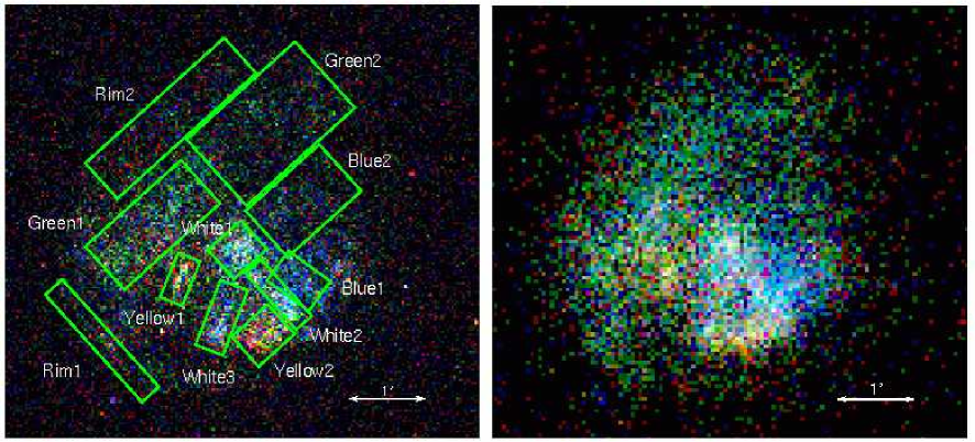
Figure 5.— Left: Three-color Chandra image of SNR G337.2$-$0.7: red, 1.0 to 1.68 keV, green, 1.68 to 2.3, blue, 2.3 to 5.0 keV (binned by 4 pixels, linearly scaled from zero to half the maximum number of counts per bin in that band). These bands were chosen because they showed the largest variations from each other. The extraction regions chosen for spectral comparisons are as marked. Right: A three-color image from $XMM$-$Newton$ MOS1 and MOS2, using the same three energy bands, but square-root scaling.

Our NEI fits require that the ratio of Ca to Si is at least 3.4${}^{+0.8}_{-0.75}$ times the solar value (Anders & Grevesse, 1989) at the 99% confidence level. However, this is only true if our model assumptions hold; i.e. that the SNR can be adequately described by a single $kT_{\rm e}$, single final $n_{\rm e}t$, planar shock. Density and composition profiles in the ejecta, instabilities both in the explosion and in the SNR evolution, and profiles or inhomogeneities in the ambient medium, should translate into different temperatures, densities, and timescales as a function of position (and composition) throughout the remnant. Such variations are suggested by the clumpy morphology of G337.2$-$0.7 in the X-ray band, an anchor-shaped bright region to the south surrounded by smoother, more diffuse emission. To test the adequacy of our single planar shock model, we first investigated how far individual regions deviate from the globally averaged spectrum.

6. X-ray Spectral Analysis: Spatial Variations within the Remnant

A comparison of images in small energy bands was used to identify possible areas of spectral variation. Spectra from these regions were first modeled independently of the global spectrum, each with a single temperature, single timescale, variable abundance planar shock model. Even in these sub-sections of the remnant, the planar shock models might not be representative of the real conditions in the ejecta, but the uniformity of model assumptions allows for fair internal comparisons between regions and to the global fitted parameters. The individual variable-abundance fits are used to compare the electron temperatures, ionization timescales and [Ca/Si] ratios throughout the remnant independent of the global fit. Alternatively, we can test if plasma conditions alone are sufficient to explain the variations by fixing the relative abundances to the values found in the global fit and allowing only the temperature, absorbing column density and ionization timescale to vary. The aim of this search is twofold, first to identify inhomogeneities in the SNR, but also to test if modeling the sum of these disparate regions with a single temperature, timescale and abundance set has biased our results.

6.1. Extraction Regions

Spectra extracted from the entire low-surface-brightness region show no obvious spectral differences from a spectrum containing all the high-surface-brightness clumps, hence surface-brightness by itself is not a good criteria for identifying spectrally distinct regions in G337.2$-$0.7. Instead, narrow energy-band images from each instrument were examined separately to identify any spectral variations across the SNR. Each event-file was divided into small spectral bins covering individual lines and areas of continuum emission identified in the overall SNR spectrum. Images in these bins were compared to look for energy bands whose images differed strongly from each other. Energy bands that were indistinguishable spatially were combined for greater signal to noise. The three energy bands that showed the greatest amount of variability from each other are displayed in Figure 5, 1.0 to 1.68 keV (red) 1.68 to 2.3 keV (green) and 2.3 to 5.0 keV (blue). This three-color image of G337.2$-$0.7 separates the energy range rich in Si and S lines (green) from the harder, more continuum dominated, regime (blue) and the soft band (red) which may include contributions from Ne, Mg, or Fe-L. The largest fluctuations in color are within the bright regions, but similar variability in the more diffuse region should not be ruled out, since it might simply be missed at this level of signal to noise. The differences seen within the bright region must be real features since they are repeated in both the $XMM$-$Newton$ and Chandra observations.

Eleven regions were chosen on the basis of their colors in Figure 5: “blue1,” “blue2,” “green1,” “green2,”“rim1,” “rim2,” “white1,” “white2,” “white3,” “yellow1,” and “yellow2.” Spectra were extracted from these regions for each instrument, and individual response matrices and ancillary response files were constructed using standard XMM-SAS and CIAO tools. Their spectra are shown in Figure 6. All exhibit strong Si and S lines indicative of enhanced abundances, but variations in conditions are evident in the relative strength of the He-like line complex and the H-like line of each species. For instance “green2” shows little or no evidence of any H-like Si, as opposed to “white1” where the 2.006 keV line from H-like Si is relatively strong. Because the regions were chosen to isolate potential spectral differences indicated by our image analysis, they do not all have similar numbers of counts. Hence not all spectra can constrain the abundances equally well.

Figure 6.— Spectra of eleven small regions around the SNR. In the NEI models shown here, the elemental abundance ratios were fixed to those found in the global SNR fit, without an additional power-law component. The spectra from all three $XMM$-$Newton$ instruments and Chandra ACIS-S3 were used in constraining the best fit model, but only the $XMM$-$Newton$ EPIC PN spectra, which have the highest signal-to-noise, are plotted here for clarity.

As before, the spectra were fit with a single component NEI model, with a variable electron temperature, ionization timescale and column density. For each region we first determined which elements required non-solar abundances as measured by the F-test for the addition of a new parameter. All regions showed significant signs of Si and S enhancement, and many (blue1, blue2, green1, green2, white1, white2) required an overabundance of Ca. No regions had statistics sufficient to determine the Ne, Mg, Ar, or Fe abundances compared to their solar values or constrain an additional power-law component. However, some do appear to have stronger Mg lines than others.

6.2. Two Approaches and their Results

In order to directly compare abundance measurements between regions, their spectra must be modeled under identical assumptions. Since the most interesting results from the global fits were those of Si, S and Ca, we chose to fit all regions with only those abundances free (all parameters, Table 2, selected values repeated in Table 3). Overall, the fitted abundances of Si, S, and Ca are super-solar but tend to be slightly lower than in the global spectrum — probably because no power-law component was included in the small region fits. At 1$\sigma$ the fitted parameters indicate variation in the electron temperatures ($0.61^{+0.11}_{-0.07}$ keV “rim1” to $1.17\pm 0.04$ keV “blue1”), logarithmic timescales ($11.09^{+0.17}_{-0.15}$ log(cm^-3s) “rim2” to fully equilibrated, $13.0_{-0.8}$ log(cm^-3s) “white2”), and the [Ca/Si] abundance ratio ($1.9\pm 0.5$ “blue1” to $4.0\pm 0.8$ “white2”). The detection of variations in the plasma parameters holds at a much higher significance level than that of the abundances. Also note that the fitted temperatures and [Ca/Si] ratios do not appear to be correlated given that 7 out of 11 best-fit [Ca/Si] ratios lie between 3.69 and 4.22 over a wide range of temperatures. From these fits it is clear that inhomogeneities in the conditions of the emitting material exist.

Table 2Fits for small regions in G337.2$-$0.7 

Region	$N_{H}$	$kT_{\rm e}$	log($n_{\rm e}t$)	Si	S	Ca	[Ca/Si]
	($10^{22}$ cm-2)	(keV)	(log(cm-3s)
rim1	3.65 (3.41–3.94)	0.61 (0.54–0.72)	11.67 (11.11–12.32)	1.50 (1.24–1.84)	2.34 (1.93–3.03)	11.76 (0–40.7)	7.84 ($<30$)
rim2	3.35 (3.21–3.55)	0.82 (0.72–0.87)	11.09 (10.94–11.26)	2.19 (1.95–2.40)	3.27 (2.89–3.86)	9.25 (1.94–16.93)	4.22 (0.9–8.6)
white1	3.01 (2.90–3.09)	0.93 (0.91–0.95)	12.0 (11.77–12.56)	3.04 (2.80–3.32)	4.13 (3.80–4.55)	11.2 (9.02–13.58)	3.69 (3.0–4.5)
white2	3.36 (3.20–3.46)	0.87 (0.85–1.02)	13.0 (12.20–13.00)	2.33 (2.13–2.68)	3.61 (3.31–4.08)	9.28 (7.34–11.30)	3.98 (3.15–4.8)
white3	3.02 (2.92–3.17)	0.90 (0.83–0.90)	12.50 (12.17–13.00)	2.10 (1.84–2.33)	2.59 (2.29–2.87)	5.86 (3.83–8.50)	2.79 (1.8–4.2)
blue1	3.84 (3.69–4.03)	1.17 (1.13–1.21)	12.13 (11.98–12.46)	2.78 (2.52–3.08)	3.48 (3.13–3.86)	5.28 (3.91–6.65)	1.90 (1.4–2.4)
blue2	3.59 (3.37–3.76)	1.08 (0.96–1.23)	11.41 (11.25–11.57)	2.53 (2.28–2.89)	3.24 (2.94–3.75 )	10.05 (7.6–13.1)	3.96 (2.9–5.2)
yellow1	3.37 (3.17–3.54)	0.67 (0.61–0.76)	11.48 (11.17–11.80)	1.32 (1.17–1.50)	1.31 (1.10 –1.55)	5.40 (0–15.15)	4.09 ($<12$)
yellow2	2.79 (2.69–2.89)	0.87 (0.81–0.95)	11.49 (11.36–11.64)	1.50 (1.37–1.65)	1.47 (1.30 –1.65)	5.89 (2.61–9.38)	3.93 (1.8–6.3)
green1	3.24 (3.20–3.39)	0.81 (0.74–0.85)	11.51 (11.42–11.65)	3.19 (2.93–3.39)	4.60 (4.32–4.89)	10.12 (7.76–12.69)	3.17 (2.4–4.0)
green2	3.87 (3.68–4.03)	0.77 (0.72–0.85)	11.49 (11.34–11.60)	3.63 (3.36–3.95)	4.64 (4.25–5.11)	14.60 (10.95–18.61)	4.02 (3.0–5.2)

The question at hand is whether the highly super-solar [Ca/Si] ratio found in the best-fit to the global spectrum could somehow be an artifact of naively summing spectra from regions with varying plasma conditions. The spectrum from region “blue1” indicates that there do exist areas in the remnant where the [Ca/Si] ratio is consistent with the solar ratio and inconsistent (at $1\sigma$) with the high [Ca/Si] ratio found from the global spectrum. Other than this one region, the spectra are consistent with the conclusions from the global model but are too shallow to confirm it with any degree of certainty. At best, three regions, “white1,” “white2” and “green2” have [Ca/Si] ratios that exceed 3 times solar at the 1$\sigma$ level. Hence these fits have only shown that high abundances of Ca relative to Si may exist throughout most of the remnant, but have not substantiated the argument. On the other hand, neither did we find a correlation between high [Ca/Si] ratios and high temperatures or a single region especially rich in Ca compared to Si that could account for the high Ca-K line flux in the overall spectrum.

Alternatively we can model each of the individual regions with the relative abundances found for the overall spectrum to see if any of the spectra require abundances significantly different than the overall fit or if all the variations can be fully accounted for by changes in the conditions. If we fix the relative abundances of Ne, Mg, Si, S, Ca, Ar, Fe, and Ni to the best-fit values for an NEI model of the global spectrum (without a power-law component) but allow the overall metallicity to be free, the spectra from all but one region (“yellow2”) are as well fit as they were under the previous set of assumptions (Table 3). Examining the spectrum of the discrepant region, “yellow2,” in Figure 6 it appears that much of the disagreement with the overall SNR ratios is at Ne and Mg. Using the F-statistic for the addition of 2 free parameters between the model which assumes the overall SNR abundance pattern and that which allows Si, S, and Ca to vary freely, gives a 99.98% probability that the allowing for independent abundances of Si, S, and Ca is a true improvement for this region. Given that the fixed abundance set used is not independent of the small region spectra, the F-statistic is not strictly correct and actually underestimates the significance of the reduction in $\chi^{2}$.

Table 3Small Regions modeled with overall abundance ratios

	solar abundances			abundance ratios
	except variable Si,S,Ca			fixed at global SNR values
region	$kT_{\rm e}$ (keV)	[Ca/Si]/[Ca/Si]☉	$\chi^{2}$ (d.o.f.)	$kT_{\rm e}$ (keV)	Y/YSNR	$\chi^{2}$ (d.o.f.)
rim1	0.61	7.84	121.11 (104)	0.84	0.65	123.61 (106)
rim2	0.82	4.22	308.10 (271)	1.01	1.02	307.42 (273)
white1	0.93	3.69	305.18 (241)	1.14	1.29	309.59 (243)
white2	0.87	3.98	299.26 (212)	1.16	1.09	295.76 (214)
white3	0.90	2.79	167.92 (173)	1.20	0.95	165.65 (175)
blue1	1.17	1.90	220.03 (200)	1.41	1.12	212.05 (202)
blue2	1.08	3.96	290.07 (275)	1.19	0.90	289.53 (277)
yellow1	0.67	4.09	100.04 (116)	0.81	0.42	100.12 (118)
yellow2	0.87	3.93	239.91 (205)	0.98	0.43	261.75 (207)
green1	0.81	3.17	530.43 (436)	0.92	1.55	531.24 (438)
green2	0.77	4.02	405.68 (398)	0.844	1.72	400.01 (400)

Given that the two prescriptions above identified two different regions as discrepant, we see that the conclusions of any given analysis are effected by the choice of how to treat all the abundances, not just the abundances of the elements with the most prominent lines. The “independent” fits which allowed Si, S, and Ca to vary but held all others at their solar values showed that the [Ca/Si] ratio for “yellow2” is entirely consistent with the overall SNR result despite the poorer fit around the Ne and Mg lines when one requires all abundances to follow the SNR pattern (as compared to the freely varying Si, S and Ca model). Vice versa, while the “independent” fits indicated that “blue1” has a lower [Ca/Si] ratio than the overall SNR, this spectrum is marginally better fit, $\triangle\chi^{2}=8.0$, assuming the overall abundance pattern of the SNR rather than forcing some elements to be fixed to their solar abundances. In the case of “yellow2” the abundances do not match the overall SNR, however it is not the high [Ca/Si] ratio that is the problem. In the case of “blue1” the goodness of fit to the overall SNR abundance ratio model shows that the initial result of a lower [Ca/Si] ratio was an artifact of not properly accounting for the emission from the less prominent species. However, it is not just the abundances themselves that are affected by the starting assumptions. The temperatures found using the global SNR abundance ratios are systematically higher by about 0.2 keV than when only Si, S, and Ca are freed from their solar values. This demonstrates the magnitude of inherent bias that any given assumption about the abundances can make in analyzing spectra with insufficient counts to constrain all the relevant abundances. The solution to this problem of a strong dependence on model assumptions would be a full Bayesian analysis, but G337.2$-$0.7 would not be a good test case for such a technique. For the present, the reader is urged to treat abundance measurements with caution and to test the sensitivity of their results to their underlying assumptions.

Despite variations in conditions, the average of the metallicities of the small regions compared to the overall SNR model is 1.01, or 1.14 when weighted by the total number of bins in each spectrum. Hence, at least in this instance, using a single global model has, if anything, underestimated the total abundances. Likewise the Ca to Si ratio averaged over the small regions is 3.96 times the solar ratio (or 3.77 weighted by the number of bins) which is also greater than the value of 3.09 times solar found in the global SNR fit before the inclusion of a power-law component.

6.3. Implications for the Morphology of G337.2$-$0.7

Disregarding for the moment the low significance level of any abundance variations, what would the fits to the small regions in Tables 2 and 3 imply about the X-ray and radio features discussed in Section 3? The X-ray regions that most closely follow the bright radio ring in both position and surface brightness are “yellow1” and “yellow2.” These two regions have the lowest abundances of Si, S, and Ca found in the remnant and also the lowest metallicity in the fits where the abundance ratios were fixed to the overall SNR values. Further, keeping Ne, Mg and Fe at their solar abundances produced a significantly better fit for region “yellow2” than the sub-solar overall [Mg/Si] values. Hence it is plausible to conclude that there is more swept-up material in “yellow1” and “yellow2” than elsewhere and that the bright radio ring denotes an interaction with a denser feature in the circumstellar or interstellar medium (such as a circumstellar wind if the remnant is young or an interaction with a molecular cloud if it is older) not the current position of the reverse shock. While the abundances are higher for regions “white1,” “white2,” and “white3,” the nearly equilibrated ionization timescales support the hypothesis of higher density material around the ring.

The results from the two “rim” regions are less conclusive. While “rim1” does have the third lowest abundances, it still favors a high Ca to Si ratio indicative of newly synthesized material. The larger region “rim2” shows no sign of lower abundances compared to the rest of the remnant, and the highest absolute abundances are found in the unremarkable, diffuse emission regions “green1” and “green2.” This may be indicating that the reverse shocked ejecta and the blast-wave into the ISM are no longer distinct in this remnant quite unlike other middle-aged SNRs such as DEM L71. On the other hand, if G337.2$-$0.7 lies at the upper end of our distance limits it would be far from the solar neighborhood, closer to the Galactic center where considerably more recycled material should enhance the metallicity by as much as 0.3 dex (e.g. Shaver et al., 1983; Rolleston et al., 2000). The second solution may seem simpler, but it exacerbates the problem of a super-solar Ca to Si ratio by requiring this abundance ratio to have been obtained over the multiple SN explosions that produced the metals in the current Galactic-center ISM.

6.4. Summary

In summary, the analysis of small regions throughout the remnant agree with the conclusions of metal-enhanced material and a super-solar Ca to Si ratio from the overall spectrum. While temperature and ionization timescale differences are present, abundance variations are comparatively small, as measured by planar shock models. In particular, we do not find any evidence for a pocket of hot Ca that could explain the Ca-line flux in the overall spectrum, nor do we see any strong deviations from the overall SNR abundances except in a portion of the bright ring which appears to have a greater contribution from swept up material.

7. Potential SN Models

Core-collapse and Type Ia explosions have widely different patterns of abundances that should be readily detected in the X-ray emission from their ejecta. In core-collapse explosions the explosive nuclear burning front passes through the existing hydrostatic layers of the star, burning them incompletely and leaving large quantities of intermediate products like O, Ne, Mg, Si, S, Ar and Ca. Much of the Fe-group material produced may fall back onto the compact object since these are formed at the highest temperatures and thus nearest the center, although some can be flung out to large distances as seen in Cassiopeia A (Hughes et al., 2000a). In Type Ia explosions, on the other hand, the thermonuclear burning efficiently incinerates most of the C/O white dwarf to Fe-group elements, with fewer intermediate products and some unburnt C and O. There is no compact object left behind in Type Ia’s, so all the Fe-group material is ejected. Hence, traditionally the O/Fe ratio has been used to identify SNRs as core-collapse or Type Ia explosions (although the vastly different conditions of the O and Fe layers in a Type Ia can make this fitted ratio deceiving; see Badenes et al., 2003). Here the question is whether a highly non-solar [Ca/Si] ratio could also be diagnostic of the explosion mechanism.

In core-collapse SNe, Si, S, Ar and Ca are all primarily produced in incomplete explosive oxygen burning, where their relative abundances are set to near solar values by quasi-equilibrium and do not vary significantly with conditions or mass (Woosley, Arnett, & Clayton, 1973). Highly energetic or highly asymmetric explosions have larger volumes of “$\alpha$-rich freeze-out” which produces ⁴⁴Ti and ⁴⁴Ca. However, these explosions also have extended volumes of explosive oxygen burning such that the common Si and Ca isotopes dominate the [Ca/Si] abundance ratio (e.g. Maeda et al., 2002; Kifonidis et al., 2003). For the prototypical core-collapse models of Woosley & Weaver (1995)(WW95), Rauscher et al. (2002), and Limongi & Chieffi (2003), the highest [Ca/Si] ratio found ($\sim$1.8[Ca/Si]_☉) was for the 12 $M_{\sun}$ “S12A” model of WW95, hereafter WWS12A.

For Type Ia models (e.g. Hoeflich & Khokhlov, 1996; Iwamoto et al., 1999; Badenes et al., 2003), high [Ca/Si] ratios are found in delayed detonation explosions (currently favored by the SN light-curves and spectra). In Badenes et al. (2003), the [Ca/Si] ratios of a delayed detonation, DDTe, and a pulsed delayed detonation, PDDe, model are 2.5, and 2.9 times the solar ratio, respectively. Given the stratification of the ejecta present in the one-dimensional models, the lack of observed Fe in G337.2$-$0.7 can be explained by the fact that Fe is shocked last and stays at a lower density (see Badenes et al., 2003, for a discussion). Recent 3-D deflagration models of Type Ia explosions produce a similar abundance pattern to the delayed detonation models shown here, without an arbitrary transition from deflagration to detonation (e.g. Reinecke et al., 2002; Gamezo et al., 2003; García-Senz & Bravo, 2005). However, they suffer from a shortage of intermediate-mass elements (Bravo et al., 2005) and the burnt and unburnt material are thoroughly bulk-mixed such that it would be difficult to explain the lack of Fe emission in the data.

Table 4Relative Abundances: [X/Si]/[X/Si]_☉

Ratio	G337.2$-$0.7	WWS12A	PDDe	DDTe
Ne/Si	1.19	0.13	0.0010	0.015
Mg/Si	0.50	0.13	0.0017	0.025
S/Si	1.44	1.46	1.5	1.4
Ar/Si	0.49	2.20	0.68	0.60
Ca/Si	3.40	1.8	2.9	2.5
Fe/Si	0.28	0.37	0.89	0.91

Table 4 compares the fitted abundance ratios to the total metal production from a core-collapse model, WWS12A and two Type Ia models, PDDe and DDTe (recall the caveats to such a comparison from Section 5.1). All models reproduce the S to Si ratio well. The core-collapse model matches the Fe to Si ratio well and does produce some Ne and Mg, but strongly over-predicts the production of Ar while still falling shy of the measured [Ca/Si] ratio. The [Ar/Si] and [Ca/Si] ratios are especially problematic because high production factors of Ca isotopes were accompanied by high production factors of Ar in all of the solar abundance massive star models of WW95. Both Type Ia models clearly match the Ca to Si ratio best and do not conflict as badly concerning the production of Ar. On the other hand, Fe is strongly over-predicted and Ne and Mg are strongly under-predicted by the Type Ia models. To determine the degree to which these discrepancies can be seen in the spectrum we performed fits of the global spectrum with the abundance ratios of C, N, O, Ne, Mg, S, Ar, Ca, Fe and Ni (relative to Si) fixed to the SN explosion predictions. Figure 7 compares NEI models for the spectrum that use the abundance ratios relative to Si of WWS12A or a delayed detonation (DDTe) model by Badenes et al. (2003). The deviations from the data for WWS12A are both more prominent and harder to explain away. While either model produces a good fit to the data if Ar (WWS12A) or Fe (DDTe) are allowed to vary, the stratification of Type Ia models provides a natural motivation for reducing the amount of Fe seen, whereas Ar, Ca, and Si should be primarily co-spatial in the ejecta of a core-collapse explosion. Furthermore, swept-up solar composition material will add Ne and Mg needed by both models but should not flip the sense of the Ar to Si ratio for WWS12A. Tests of a two-component model, one with solar composition (ISM) the other with freely varying abundances (ejecta) bear this out. If the temperatures of the two components are set to reasonable values (such as the blast-wave and EM-averaged Si temperatures from Section 7.1) the fitted [Ne/Si], [Mg/Si] and [Fe/Si] abundance ratios in the “ejecta” component drop steeply, while the sub-solar [Ar/Si] ratio and super-solar [Ca/Si] and [S/Si] ratios remain at values similar to the one component fit. Hence a strict comparison of the global abundance ratios clearly favors an origin as a Type Ia SN. If true, G337.2$-$0.7 would be only the third potential Ia SNR with a significantly disturbed morphology after Kepler’s SNR (e.g. Cassam-Chenaï et al., 2004) and N103B (Hughes et al., 1995; Lewis et al., 2003), both of which also have controversial identifications.

A core-collapse scenario with solar-like abundance ratios between Si, S, Ar, and Ca could still be viable if the strong Ca-K line is the result of differing plasma conditions rather than abundance. Line fluxes in general are strongly dependent on the electron temperature and ionization, hence if the temperature of the Ca-rich material were sufficiently higher than in the Si-rich ejecta this could also account for their unusual line ratio. A global fit allowing a separate temperature and ionization time-scale for Ca but holding [Ca/Si]=[Ca/Si]_☉ performs equally well as our single temperature fit with a free Ca abundance, with almost identical best-fit $\chi^{2}$ values. The electron temperature associated with the Ca emission was $1.0$ keV as compared to $0.75$ keV for the Si and other elements. However, no spatially distinct region with a high temperature and high [Ca/Si] ratio was identified in the small region fits. On the other hand, this does not preclude the possibility of two unresolved or co-existing plasmas. For instance, one could consider the case of a two density medium in pressure balance, with a single elemental composition shocked at a single time. We looked at a model with two NEI components with the same abundances, their temperatures tied at a series of fixed ratios and the ionization timescales offset appropriately for pressure balance. This did result in a sub-solar [Ne/Si] ratio ($\sim$0.8[Ne/Si]_☉) and reduced the amount of Fe required by the fit ($\sim$0.05[Fe/Si]_☉) but did not change the pattern of Si, S, Ar and Ca abundances substantially ($\sim$1.5[S/Si]_☉, $\sim$0.5[Ar/Si]_☉, $\sim$3.0[Ca/Si]_☉). Hence, although this question is not well-defined, it seems unlikely that a multi-temperature plasma with an abundance pattern typical of a core-collapse explosion could explain the global spectrum of G337.2$-$0.7 without considerable compositional differences from place to place.

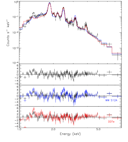
Figure 7.— Total ejected elemental masses compared to the global SNR G337.2$-$0.7 spectrum. Only the MOS 1 spectrum is shown for simplicity, although all four instruments were considered in the analysis. The original free-abundances NEI model is shown in black. For comparison the relative abundances were fixed to the appropriate ratios given the total ejected mass of each element in a core-collapse (WW S12A: blue) and a Type Ia (DDTe: red) model.

In the above discussion we have compared the global spectrum of G337.2$-$0.7 to the total metal output of the SN explosion models with the addition of a few simple two-temperatures tests and concluded that the products of a Type Ia explosion are more consistent with the spectrum. In reality the blast-wave into the ISM may contribute substantially to the total spectrum and the ejecta itself will not be a homogeneous mix of the nucleosynthesis products. Layering of the composition or large scale anisotropies imply that not all products will be visible in the X-rays at all times, nor will they be under uniform conditions. A true comparison of the global SNR spectrum to explosion models requires that the evolution of ejecta and shock fronts be followed from the time of the explosion until the present age of the remnant to predict the X-ray spectrum. While no such model is available for the variety of core-collapse models, the models of Badenes et al. (2003) provide the opportunity for exactly such a comparison for the case of a Type Ia explosion.

7.1. Investigation of Possible Type Ia Explosion Mechanisms

Many groups have produced grids of Type Ia models to compare to SN spectra and lightcurves (e.g. Hoeflich & Khokhlov, 1996; Iwamoto et al., 1999). Badenes et al. (2003) have expanded upon this work to enable comparisons to the remnants of Type Ia SNe. Badenes et al. (2003) followed the plasma conditions and ionization state within the ejecta of Type Ia SNe from the explosion itself to 5000 years later, and calculated the expected X-ray emission of the ejecta and the blast-wave for various times in the evolution of the remnant. Their network of Type Ia explosion models attempted to cover all currently debated explosion mechanisms from pure detonation (super-sonic flame propagation) to pure deflagration (sub-sonic flame propagation), as well as a sub-Chandrasekhar mass explosion. Their models showed a strong evolution of the contribution from each element to the X-ray spectrum. Indeed, for some models Fe did not begin to appear until late times.

The structure of the ejecta as prescribed by each SN Ia model will evolve as the forward shock expands out into the ambient medium and a reverse shock is generated that propagates back into the layers of ejecta. The X-ray emission from the SNR will have contributions from both the outer blast wave (reasonably approximated by a Sedov solution after on the order of 1000 years) and the reverse shock (followed in detail in the models of Badenes et al., 2003). In this simple one dimensional picture only the outermost layers will be shocked at the earliest times, and thus begin to ionize and emit in the X-rays. Elements that are only present in deeper layers will show up later in the spectrum and experience different temperatures and densities than the earlier layers.

For comparison with the spectrum of G337.2$-$0.7, for every explosion model in the grid of Badenes et al. (2003), the evolution of the SNR was computed in a grid of three ambient densities, $\rho_{am}$ (0.2, 1.0, 5.0 $\times 10^{-24}$ g cm^-3). From each of these SNR models, spectra from the shocked ejecta were extracted at four different ages (500, 1000, 2000, and 5000 years). The synthetic spectra of Badenes et al. are completely characterized by four parameters only: the Type Ia explosion model, the age of the SNR $t$, the AM density $\rho_{am}$, and the amount of collisionless heating at the reverse shock $\beta$ (defined as the ratio of electron to ion specific internal energies at the shock front). Among these parameters, we have not explored variations in the last one ($\beta$), which tend to enhance the Fe emission, and particularly the flux in the Fe K blend, due to the higher electron temperatures brought on by collisionless heating. In the case of G337.2$-$0.7, this effect is disfavored by the conspicuous absence of Fe K in the X-ray spectrum. For a discussion on collisionless electron heating at SNR shock fronts, see Rakowski (2005), for its impact on the ejecta emission, see sections 2.2 and 2.4 in Badenes et al. (2005a).

One significant advantage of the spectra of Badenes et al. (2003) is that they have an underlying physical model for the dynamics of the SNR. However, the underlying model is calculated using approximations that need to be taken into account for the comparison between the data and the synthetic spectra. One such approximation is the fact that the models are calculated in one dimension. This is clearly a simplification of a very complex situation, because deviations from spherical symmetry are expected both on theoretical grounds (the contact discontinuity between the forward and reverse shocks is subject to Rayleigh-Taylor instabilities) and due to the large scale structure observed in the X-ray images of G337.2$-$0.7 (see sections 3 and 6.3) Thus, the constraints obtained by the comparison between the spatially integrated spectrum and the one dimensional models of Badenes et al. (2003) are focused on the emission measure averaged emission of the SNR (i.e., they tend to reflect the properties of the brightest regions). Local deviations in the properties of the ejecta and blast wave emission from the best-fit synthetic spectrum are expected, but the average properties of the plasma should be similar to those of the most successful models. Since we consider the emission from all the elements at the same time, it is unlikely that this kind of local deviations would conspire to affect our choice of models, but this possibility cannot be ruled out completely. Another important approximation in the models is that the ambient medium is assumed to have a uniform density. Again, this is just a simplification of a complex scenario. Theoretical studies indicate that the circumstellar medium around a Type Ia SN should be strongly modified by the pre-supernova evolution of its binary progenitor, which would sculpt a bubble-like cavity (Badenes & Bravo, 2001). This should affect the dynamics of the subsequent SNR (Dwarkadas, 2000), but the observations of prototype Type Ia SNRs like Tycho or SN1006 show no evidence for such strongly modified dynamics (Badenes & Bravo, 2001, , see also Badenes 2004, PhD thesis). On the other hand, the fact that Type Ia SNe are not detected in the radio (Weiler et al., 1989), or X-rays (Schlegel & Petre, 1993) seems to indicate that the impact of the progenitor evolution on the circumstellar medium is limited. Only two Type Ia SNe have shown signs of H$\alpha$ emission from interaction with circumstellar material 2002ic (Hamuy et al., 2003) and 2005gj (Prieto et al., 2005). In the absence of strong evidence to the contrary, we consider the constant ambient density hypothesis as a valid approximation, and we note that if this were not the case, our detailed comparisons might need to be revised. For reference, given emission-measure and metallicity considerations, the density of the total ambient medium swept-up in the ring is about twice that of the diffuse emission (see Dwarkadas, 2005, for discussions of how the mass and radius of a wind shell might effect the dynamics of the SNR).

The spectra were calculated using a plasma emission code maintained by K. Borkowski, whose inputs are the electron temperature and ionization structure of each ejecta layer as predicted by the SNR model (see Badenes et al., 2003, for details). An additional Sedov component appropriate for the specified age, ambient density and explosion energy was used to model the blast-wave contribution. The version of the emission code used here is missing calculations for Argon as well as some of the Li-like lines for other elements that can be important for material far from ionization equilibrium. (These were included in the NEI code used in the previous section.) In particular we believe the disagreement in the line centroid for Ca in the upcoming comparisons is an artifact of the atomic data used in this NEI emission code. However, for the purpose of comparing the models with the observed global spectra, over a discrete grid in density and age, these emission models were the most straightforward to use and readily available to the community. Only the normalization and absorbing column density are allowed to vary to find the best fit for each grid point.

The $\chi^{2}$ statistic is inappropriate for these comparisons since we are not allowing the parameters to vary freely. These models have a more limited range of flexibility to fit the observations than the general NEI fits used before given that the evolution and abundance pattern are entirely constrained. However, we can still use the best-fit $\chi^{2}$ value at each grid point as a quantitative guide for which models are a closer match. It is also useful to record the $\chi^{2}$ value over energy bands within the spectrum to confirm our suspicions based on visual inspection of why a certain age and density is “fitting” well or poorly. These numbers are not of rigorous statistical value, but rather just a rough measure of which models are good matches and why.

Just like the fits presented in Section 5, the goal is to match the abundances, ionization state and temperature of the observed spectrum. However in this case, with two connected but separately evolving components, matching the data is a matter of finding the best balance of these components for any given model. For a given density, as time progresses the Sedov component becomes more dominant, reducing the apparent equivalent widths of the metal lines, and the blast-wave component also cools, eventually to below the temperature we measured in the last section. Meanwhile the ejecta component is also evolving. The reverse shock is penetrating deeper into the layers of nucleosynthetic products, and the already-shocked material is continuing to equilibrate in temperature and ionize.

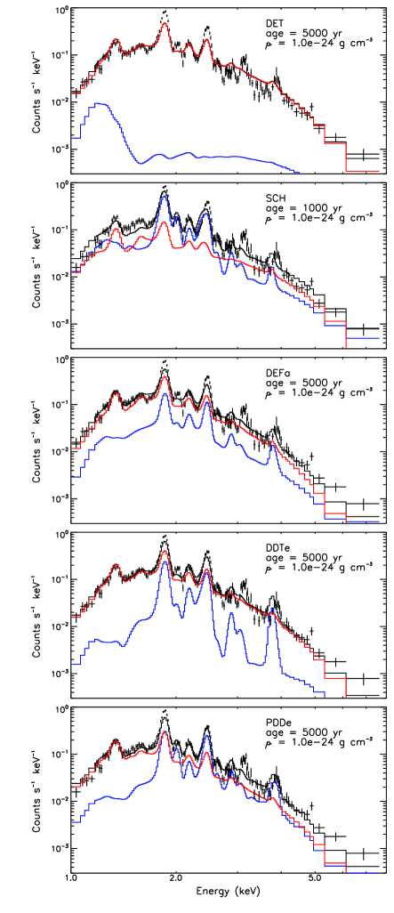
Figure 8.— Type Ia SNR model comparisons over the original grid of densities and ages. The blast-wave (red) and ejecta (blue) both contribute to the overall model spectrum (black). The closest matches for each explosion type are plotted here against just the MOS1 data for clarity. From top to bottom, DET pure detonation, $\rho_{am}=1.0\times 10^{-24}$ g cm^-3, age = 5000 years; SCH sub-Chandrasekhar, $\rho_{am}=1.0\times 10^{-24}$ g cm^-3, age = 1000 years. DEFa pure deflagration, $\rho_{am}=1.0\times 10^{-24}$ g cm^-3, age = 5000 years. DDTe, delayed detonation, $\rho_{am}=1.0\times 10^{-24}$ g cm^-3, age = 5000 years and PDDe, pulsed delayed detonation, $\rho_{am}=1.0\times 10^{-24}$ g cm^-3, age = 5000 years. The bottom two panels show the delayed detonation models that are a better match to the continuum shape, line fluxes and ionization state than the others.

The first test a model must pass is whether there is a time when the abundance pattern of the ejecta (modified by the solar abundance contribution for the blast wave) matches that inferred from the data and the relevant emission lines are of appropriate strength relative to the continuum (from both the Sedov and ejecta components). Three explosion models can be rejected from this consideration alone (see Table 5). A pure detonation explosion (DET) efficiently burns all material to Fe-group elements as it propagates supersonically through the white dwarf, leaving only a thin skin of intermediate elements before it is quenched in the outer layers. Thus for DET the iron produced always dominates the Si, S, and Ca present in the spectrum, entirely unlike the lack of iron (relative to most Ia models) found in G337.2$-$0.7. The closest match occurs once the solar abundance ambient medium is dominating (Figure 8a) which we already know cannot produce strong enough lines to reproduce the spectrum.

In the sub-Chandrasekhar model (SCH) a detonation originates on the surface of the star and burns the outer layers of accreted material. When the ensuing pressure waves converge on the center of the WD, a second ignition happens and a detonation propagates back out. Both the center and the outside of the star are incinerated to Fe-group elements, while the middle region is less completely burned. For SCH, there simply isn’t a time at which the abundance pattern is a good match for G337.2$-$0.7. Prior to $\sim$1000 years the Sedov component is insufficient to fill in the soft continuum. Around $\sim$1000 years the Si lines are reasonably well matched in ionization state and strength relative to the continuum (see Figure 8b) but no other portion of the spectrum is well-modeled at this time. After $\sim$1000 years the Si and S ejecta are swamped by the Sedov component. This blast-wave dominated nature occurs earlier for the SCH models than it does for the other Type Ia models because of the low ejected mass and explosion energy.

The pure deflagration models (DEF) are also a poor match to the spectrum of G337.2$-$0.7. Here the flame front is sub-sonic, and the the star expands in reaction to the flame propagating out from the center. The flame is quenched in the outer regions when the expansion of the material is of the same order as the flame velocity. This front burns the interior efficiently to Fe-group elements but leaves a large portion of unburnt C and O in the outer layers. The high column density to G337.2$-$0.7  masks the emission lines of carbon and oxygen so that the preponderance of this unburnt material in the pure deflagration models manifests itself as strong continuum emission from 1 to 8 keV. Thus even within the ejecta component the equivalent widths of Si, S, and Ca are fairly low. The Si-rich material lies deep enough in the star that by the time Si emission is prominent the Sedov contribution is starting to dominate (Figure 8c). Furthermore since it has been shocked relatively recently the ionization state of Si is not sufficiently advanced. Soon after the DEF “best match” the Sedov contribution dominates and the Fe-K emission becomes too prominent as well. Simulations with a finer grid in ambient density and age for the SCH and DEF models did not improve upon the fits shown in Figure 8.

The remaining viable models are the delayed detonation and pulsed delayed detonation models, DDT and PDD, that were preferred initially because of the likeness of their overall abundance pattern to that of G337.2$-$0.7. In delayed detonation models, the flame begins at the center as a deflagration, briefly forcing the expansion of the star, but at some prescribed flame density it transitions to a detonation front. Like the DEF models the center is efficiently burned to Fe-group elements, but due to the initial expansion the detonation burning in the outer layers encounters a wider region where intermediate mass elements can be produced before the flame is quenched. Thus there is a shell of Si-rich material outside the Fe-rich core. The PDD models invoke a pulsation of the star to induce the transition from deflagration to detonation. They produce a similar pattern of elemental production to DDT with a modified density structure. In both cases a range of transition densities were explored, with the models labeled from a to e in order of the earliest to the latest transitions from deflagration to detonation.

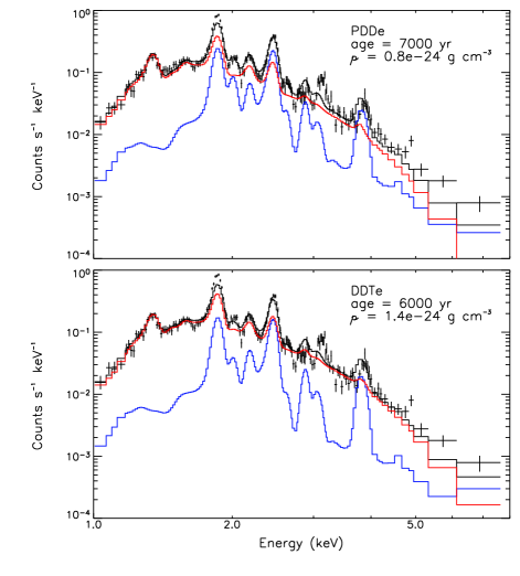
Figure 9.— The “best match” models for DDTe and PDDe over a finer grid of densities and ages. As in Figure 8, the blast-wave (red) and ejecta (blue) both contribute to the overall spectrum (black). For DDTe $\rho_{am}=1.4\times 10^{-24}$ g cm^-3, age = 6000 year. For PDDe $\rho_{am}=0.8\times 10^{-24}$ g cm^-3, age = 7000 year. Only the MOS 1 spectrum, which has the highest spectral resolution around the Si line-complex, is shown, although all four instruments were considered in the analysis.

As seen in the previous section, the primary disagreement between the overall elemental production and the inferred abundances in G337.2$-$0.7 was the over-prediction of Fe. Since the Fe is produced primarily in the more interior portion of the star in either delayed detonation model, it is possible that the computed emission from Badenes’ models might more accurately match the G337.2$-$0.7 spectrum than the naive comparison to the total elemental production. As expected, amongst the delayed detonation models, PDDe and DDTe that produce the least amount of Fe, are preferred over their more energetic cousins when comparing their predicted spectra with that of G337.2$-$0.7. In fact both PDDe and DDTe have fairly good matches to the G337.2$-$0.7 spectra at an ambient density of $1.0\times 10^{24}$ g cm^-3 and an age of 5000 years (Table 5, Figure 8d and e). In comparison to the DET, SCH, and DEF models that have “failed”, the delayed detonation models produce stronger Si, S, and Ca lines at the appropriate ionization stage than any of the others at close to the right “abundance” ratios. The S lines are quite well matched and Si is under-predicted but less so than in DEF or DET. At this stage, the reverse shock has actually penetrated fully through the ejecta, but the Fe remains “hidden” due to a lower electron temperature and ionization timescale (see below for details) and the dominance of the blast-wave component.

Table 5Best “matches” for each Type Ia model

model	$\rho_{am}$	age	$r_{fwd}$	$D_{r}$	$N_{\rm H}$	norm	$D_{norm}$	$\chi^{2}$
	$10^{-24}$ g cm-3	years	pc	kpc	$10^{22}$ cm-2	(at 10kpc)	kpc	(just MOS2)
DET	1.0	5000	12.2	15.5–18.2	3.96	0.73	11.7	1247.31
DEFa	1.0	5000	9.8	12.5–14.6	4.12	1.99	7.1	786.44
SCH	1.0	1000	5.7	7.3–8.5	3.17	1.4	8.4	795.15
PDDe	1.0	5000	11.7	14.9–17.5	3.22	0.44	15.1	672.26
DDTe	1.0	5000	11.5	14.6–17.2	3.78	0.77	11.4	701.68
PDDe	0.8	7000	14.0	17.8–20.9	3.75	0.94	10.3	549.33
DDTe	1.4	6000	11.5	14.6–17.2	3.80	0.53	13.7	627.66

The next question is whether there is an age and density where the apparent ionization state of Si, S, and Ca are reached before the Sedov component swamps the ejecta component. To evaluate this requires examining a more densely spaced grid in ambient density and age. For PDDe, the $\rho_{am}=1.0\times 10^{24}$ g cm^-3 model, at 5000 years appeared to be very close to the correct ionization timescale, but possibly under-abundant in Si, S and Ca. Hence we looked to slightly lower densities where the Sedov solution would take longer to become dominant, but towards longer times so that the model would reach the same ionization stage ($\rho_{am}=0.8,0.9,1.0\times 10^{24}$ g cm^-3 , age = 5000, 6000, 7000, 8000 years). For DDTe at an ambient density of $1.0\times 10^{24}$ g cm^-3 and age of 5000 years, the ionization state of Si and S both appear too young. There is no evidence for a H-like Si component above the Sedov continuum. Hence we looked to slightly higher densities and ages around 5000 years for a better match ($\rho_{am}=1.2,1.4,1.6,1.8\times 10^{24}$ g cm^-3, age = 4000, 5000, 6000, 7000 years). For all these models, a post-facto test of the importance of cooling shows that neglecting radiation is a valid approximation for these densities and ages.

Using the $\chi^{2}$ value relative to all three $XMM$-$Newton$ spectra (MOS1, MOS2 and PN) as a guide we find a best match for PDDe at $\rho_{am}=0.8\times 10^{24}$ g cm^-3, age = 7000 years ($\chi^{2}$ = 2287) and for DDTe at $\rho_{am}=1.4\times 10^{24}$ g cm^-3, age = 6000 years ($\chi^{2}$ = 2526) as shown in Figure 9 (the implications of these particular parameters will be discussed shortly). Given that the only variables in these models are the ambient density, the age and the absorbing column density, these are remarkably good matches for the character of the G337.2$-$0.7 spectrum. While the Si abundance or flux in the He-like Si K-shell lines ($\sim$1.86 keV) are less than they should be, the H-like Si Ly$\alpha$(2.0 keV) and Ly$\beta$(2.37 keV) are well matched by the combination of the blast-wave and ejecta components. S and Ca are primarily contributed from the ejecta component. Both compare well with the data in flux, and S appears to agree in ionization state as well. Ne, Mg and the soft continuum are dominated and well-modeled by the blast-wave. The hard end of the continuum is slightly under-predicted but no strong Fe-K line from the ejecta is found that would disagree with the G337.2$-$0.7 spectrum. Comparing to the previous figure, the failures in the other models may become clearer. Once the first requirement was met, i.e. the lack of a prominent Fe-K line, the most diagnostic aspects of the spectrum were the soft-continuum, H-like Si-K, and the S and Ca abundances.

The relative contributions from the blast wave and ejecta to individual spectral features are also interesting to note in light of our previous discussions on the interpretation of the global and small region spectra. In particular the best-matched delayed detonation models attribute essentially all of the Ne and Mg line emission to the solar-composition blast wave component, exactly in line with our explanation for their abundances in the global fits. This is also in keeping with the interpretation of the bright ring as a circumstellar interaction given that the Ne and Mg emission from region ”yellow2” preferred solar abundances as opposed to the sub-solar abundances relative to Si seen in the remnant as a whole.

Table 6Electron Temperatures and Ionization Timescales
for Two of the Type Ia Models

	Sedov	Ejecta
		Si	Ca	Fe
PDDe
$kT_{\rm e}$ (keV)	0.69	1.68	1.83	1.60
log($n_{\rm e}t$) log(cm-3s)	11.58	11.12	10.63	10.26
DDTe
$kT_{\rm e}$ (keV)	0.65	2.11	2.11	1.82
log($n_{\rm e}t$) log(cm-3s)	11.76	10.53	10.53	10.27

Given that the line fluxes, continuum shape and apparent abundances here are the sum of multiple components, how do the electron temperatures and ionization timescales compare with our naive single NEI model? Table 6 lists the temperatures and ionization timescales for the Sedov blast-wave component and selected elements at the specific age and ambient density that best-match the spectrum of G337.2$-$0.7. The parameters listed for the ejecta are the EM weighted averages of the electron temperatures and ionization timescales in the regions containing those elements. Given the evolutionary state implied by the ambient density and ages found here it is not surprising that fits to the global spectrum reflect the blast-wave more than the ejecta. The temperatures and timescales we measured under the assumption of a single $kT_{\rm e}$ and $n_{\rm e}t$ most closely approximate the Sedov component of the Type Ia SNR models, but may have been pushed towards higher values of $kT_{\rm e}$ and $n_{\rm e}t$ by the bright hot ejecta. Naively one might worry that the stratified abundance pattern that minimizes the Fe-K line flux would also imply that the Ca should be under significantly different plasma conditions than Si. However, the EM averaged temperatures and ionization timescales for Ca and Si are actually quite similar to each other in PDDe, and almost identical in DDTe because these elements are largely co-spatial in the ejecta (see Table 6). On the other hand, the EM averaged quantities for Fe are quite different from Si, especially given that both the lower electron temperature and the shorter ionization timescale imply a lower level of ionization. These differences combined with the relative dominance of the blast-wave component allows the Fe to remain hidden. None of the ionization timescales in these Type Ia SNR models reach the value from the single temperature NEI model, however the Sedov ionization timescales are quite similar to the values found in the fainter small regions outside the bright ring.

Badenes’s Type Ia SNR models naturally provide two determinations of the distance to the SNR by predicting both the radius of the outer-blast-wave, which can be compared to the angular size of the radio SNR, and the EM normalized to a nominal distance of 10 kpc. Comparing the two distance estimates for a single Type Ia model (Table 5) we see that they are at least grossly comparable with each other (not surprising given that the angular size used is from the faint material, while the normalization is largely due to the bright material). The distances estimated here for the PDDe and DDTe models from the normalization and radius are larger than but similar to the upper limit on the distance from the H I absorption measurements. Also note that the ages and densities of the best-matched Type Ia models are roughly the same as those estimated in Section 5.3 for the far end of the allowed distance range. However, unlike the estimates in Section 5.3 which only considered emission from the blast-wave, here the ejecta component is explicitly considered and a pre-defined explosion energy has been set. In fact these ages and ambient densities were primarily chosen to match the relative importance of Sedov and ejecta components seen in the spectrum. Given a reasonable distance estimate of 10 kpc the radius of the bright ring would then be 4.6 pc. While this is considerably larger than a typical planetary nebula, it is actually quite similar to the size of some of the largest planetary nebula with measured parallaxes (Borkowski et al., 1990), consistent with the interpretation of the ring as an interaction with a structure in the circumstellar medium.

Simply increasing the ambient density to increase the ionization timescale and decrease the radius will not solve the remaining discrepancy in distance because an increased density also results in an increased luminosity which in turn implies a larger distance to the SNR (explained in detail by Badenes et al., 2005b). However, the history of the remnant is not likely to be as simple as we have modeled. Radiative losses to the shock, energy lost from the escape of cosmic-rays, the blast-wave running into a dense circumstellar ring of material or ambient cloud, would all be consistent with a decreased inferred shock energy, a higher timescale and a smaller radius. It is likely that more than one of these has occurred given that roughly three quarters of the explosion energy would need to be dissipated to explain the discrepancy between the Type Ia models and the H I distance range. If on the other hand general absorption in the region around G337.2$-$0.7 has obscured a true absorption feature at $-116$km s^-1 then no modification is required and we are left with a best estimate of the distance from the X-ray spectrum and radio extent alone.

8. Conclusions

The line-rich thermal ASCA X-ray spectrum of SNR G337.2$-$0.7 identified it as an “ejecta-dominated” remnant (Rakowski et al., 2001). In this paper we examine the new $XMM$-$Newton$, Chandra, and ATCA observations of G337.2$-$0.7 to learn as much as possible about its progenitor system.

The radio observations provide an image of the full extent of the remnant. At both 1.4 and 5 GHz the remnant exhibits diffuse emission throughout a shell 2.3′$\times$ 2.7′ in radius that is limb-brightened in some places but not in others. In the interior lies a bright elliptical ring of radio emission that must indicate a local increase in either density or magnetic field (or both). Compared to the X-rays, we see at least one outer-rim radio filament with X-ray emission, and there is bright X-ray emission related to the radio ring but brightest in different places. Radio H I absorption measurements also provide a constraint on the distance of between $2.0\pm 0.5$ kpc and $9.3\pm 0.3$ kpc.

The X-ray spectrum of SNR G337.2$-$0.7 has been studied in detail both globally and locally. Starting from a single temperature NEI planar shock model for the spectrum of the whole remnant, the previously seen super-solar abundances of Si and S are confirmed and further constrained ($3.50^{+0.24}_{-0.62}$ and $5.04^{+0.32}_{-0.82}$ times their solar abundances, respectively). The most striking new features of $XMM$-$Newton$ and Chandra spectra are a strong Ca K-shell line, and the lack of any significant K-shell line from Fe. The lack of an Fe-K line implies that the soft X-ray spectrum is coming from a cooler bremsstrahlung continuum plus a Mg-K line, rather than unresolved Fe-L lines as previously argued by Rakowski et al. (2001). The strong Ca line indicates the presence of Ca-rich ejecta, yielding a Ca abundance of almost 12 times the solar value in the single temperature, single timescale model. Moreover the global spectrum requires a [Ca/Si] ratio of at least $2.65$ times solar at the 99% confidence level. In contrast, the [Ar/Si] ratio is found to be sub-solar.

We looked for but could not find any evidence to doubt the abundance pattern of Si, S, Ar, and Ca found in the single temperature model. Spectra from small regions around the remnant showed variations in electron temperature and ionization timescale but no clear evidence for variations in the abundance pattern. The abundances in the bright radio ring are if anything lower than the surrounding areas indicating an origin in the circumstellar medium. For the global spectrum two additional simple two-temperature models were explored, one with abundances tied across components and one that had a solar composition plasma in addition to the freely varying one. These differed from the single temperature model in the relative abundances of Ne, Mg or Fe but not of Si, S, Ar, and Ca.

The abundance pattern seen in the global spectrum strongly favors a Type Ia origin. The composition and stratification of the ejecta in delayed-detonation Type Ia models can explain the overall abundance pattern if the contribution from a solar composition blast-wave into the ISM is included and the reverse shock has only recently reached the bulk of the Fe-group ejecta. On the other hand, typical core-collapse explosions produce Si-group elements in the same nuclear burning processes and at approximately their solar ratios, inconsistent with the abundances of our single temperature global SNR model. Core-collapse explosion models that do have a highly super-solar [Ca/Si] also have super-solar [Ar/Si] ratios, the opposite of which is seen in G337.2$-$0.7. The only remaining viable explanation for a core-collapse model is if a significant amount of hot Ca-rich material is segregated from the bulk of the Si-rich plasma. Our examination of small regions throughout the remnant cannot exclude this possibility especially if the two plasmas were unresolved but no spatially distinct hot region with a significantly high [Ca/Si] ratio was found.

As emphasized above, a single temperature model is inherently overly simplistic in that it does not reflect the variations in composition and conditions within a SNR either between the blast-wave and the reverse-shocked ejecta or within the ejecta itself. Given that our initial results support an origin in a Type Ia SNe and that Badenes et al. (2003) have produced predicted spectra from Type Ia SNRs, we have the opportunity to test whether our conclusions hold when actual conditions are taken into account. Simulated spectra from a variety of Type Ia explosion models were compared with the global spectrum of G337.2$-$0.7 to find the ambient density and age for each model that best matches the spectrum, i.e. that avoids a strong Fe-K line, reproduces the strength of the He-like Si-K lines relative to the continuum, exhibits bright S and Ca lines, and reflects the line shapes and line-ratios within a given element. In the end we saw that indeed Type Ia models that did not initially match the fitted abundances in total metal production also did not match the spectrum at any special time in their evolution. The preferred delayed detonation and pulsed delayed detonation models could in fact reproduce the generic features of the G337.2$-$0.7 spectrum. In these simulated spectra the reverse shock has over-run the Fe-rich material, but there is still no strong Fe-K line because Fe is at a lower EM-weighted average temperature than the other elements and the high energy X-ray band is dominated by blast-wave continuum emission.

From the above analyses combined with distance constraints from the radio data, we are also able to infer the current evolutionary state of G337.2$-$0.7. Simple Sedov estimates from the single temperature, single timescale fits yield ages of between 750 and 3500 years. For the Type Ia SNR models of Badenes et al. (2003), based on the relative contributions of the interstellar material and the ejecta, G337.2$-$0.7 is about 5000 years old. Both the age and normalization of the Type Ia SNR models imply that G337.2$-$0.7 is probably toward the upper limit of its allowed distance range. Hence, while G337.2$-$0.7 may not be “ejecta-dominated” in a literal sense, even after 5000 years and with more than 50 $M_{\sun}$ of swept up material, G337.2$-$0.7 still exhibits clear evidence of ejecta.

To reiterate the main purpose of the paper, analysis of the X-ray spectrum of G337.2$-$0.7 have allowed us to identify it as a Type Ia remnant and, if our identification is correct, show that low-energy (Fe-poor) delayed detonations or pulsating delayed detonations are the preferred explosion mechanisms. The conspicuous absence of Fe K emission in the X-ray spectrum is a strong indication that little Fe is found in the outermost layers of SN ejecta, where it would be revealed by the high densities and electron temperatures. This precludes any Type Ia SN model with plumes of Fe (⁵⁶Ni) at high velocities, including sub-Chandrasekhar explosions and three dimensional deflagrations with well-mixed ejecta. We also find that the bright ring of radio emission is likely to be evidence of the impact of the Type Ia progenitor system on the circumstellar medium. In the case of G337.2$-$0.7, the high [Ca/Si] ratio, combined with a low [Ar/Si] ratio found in the single ionization, single electron temperature models, did indeed point to a Type Ia origin - a scenario which then was shown to be viable under a more detailed scrutiny. However, the low abundance of Fe, which one might have expected to have come from a core-collapse explosion, was actually a red-herring, and could be explained in the Type Ia scenarios once actual conditions within the ejecta were taken into account.

References

- Akiyama et al. (2003) Akiyama, S., Wheeler, J. C., Meier, D. L., & Lichtenstadt, I. 2003, ApJ, 584, 954
- Anders & Grevesse (1989) Anders, E. & Grevesse, N. 1989, Geochim. Cosmochim. Acta, 53, 197
- Arnaud (1996) Arnaud, K. A. 1996, in ASP Conf. Ser. 101: Astronomical Data Analysis Software and Systems V, 17–+
- Badenes et al. (2005a) Badenes, C., Borkowski, K. J., & Bravo, E. 2005a, ApJ, 624, 198
- Badenes et al. (2005b) Badenes, C., Borkowski, K. J., Hughes, J. P., Hwang, U., & Bravo, E. 2005b, ApJ, in press (astro-ph/0511140)
- Badenes & Bravo (2001) Badenes, C. & Bravo, E. 2001, ApJ, 556, L41
- Badenes et al. (2003) Badenes, C., Bravo, E., Borkowski, K. J., & Domínguez, I. 2003, ApJ, 593, 358
- Bell et al. (2004a) Bell, J. B., Day, M. S., Rendleman, C. A., Woosley, S. E., & Zingale, M. 2004a, ApJ, 606, 1029
- Bell et al. (2004b) —. 2004b, ApJ, 608, 883
- Borkowski et al. (1990) Borkowski, K. J., Sarazin, C. L., & Soker, N. 1990, ApJ, 360, 173
- Branch et al. (2005) Branch, D., Baron, E., Hall, N., Melakayil, M., & Parrent, J. 2005, PASP, 117, 545
- Bravo et al. (2005) Bravo, E., Badenes, C., & García-Senz, D. 2005, in AIP Conf. Proc. 797: Interacting Binaries: Accretion, Evolution, and Outcomes, 453–462
- Burrows et al. (1995) Burrows, A., Hayes, J., & Fryxell, B. A. 1995, ApJ, 450, 830
- Burrows et al. (2005) Burrows, A., Walder, R., Ott, C. D., & Livne, E. 2005, in ASP Conf. Ser. 332: The Fate of the Most Massive Stars, 358–+
- Cassam-Chenaï et al. (2004) Cassam-Chenaï, G., Decourchelle, A., Ballet, J., Hwang, U., Hughes, J. P., Petre, R., & et al. 2004, A&A, 414, 545
- Corbel et al. (1999) Corbel, S., Chapuis, S., Dame, T. M., & Durouchoux, P. 1999, ApJ, 526, L29
- Dame et al. (2001) Dame, T. M., Hartmann, D., & Thaddeus, P. 2001, ApJ, 547, 792
- Dwarkadas (2000) Dwarkadas, V. V. 2000, ApJ, 541, 418
- Dwarkadas (2005) —. 2005, ApJ, 630, 892
- Fich et al. (1989) Fich, M., L., B., & Stark, A. A. 1989, ApJ, 342, 272
- Frater et al. (1992) Frater, R. H., Brooks, J. W., & Whiteoak, J. B. 1992, J. Electr. Electron. Eng. Aust., 12, 103
- Fryer & Heger (2000) Fryer, C. L. & Heger, A. 2000, ApJ, 541, 1033
- Gamezo et al. (2003) Gamezo, V. N., Khokhlov, A. M., Oran, E. S., Chtchelkanova, A. Y., & Rosenberg, R. O. 2003, Science, 299, 77
- García-Senz & Bravo (2005) García-Senz, D. & Bravo, E. 2005, A&A, 430, 585
- Green et al. (1999) Green, A. J., Cram, L. E., Large, M. I., & Ye, T. 1999, ApJS, 122, 207
- Hamilton et al. (1997) Hamilton, A. J. S., Fesen, R. A., Wu, C.-C., Crenshaw, D. M., & Sarazin, C. L. 1997, ApJ, 481, 838
- Hamuy et al. (2003) Hamuy, M., Phillips, M. M., Suntzeff, N. B., Maza, J., González, L. E., Roth, M., Krisciunas, K., Morrell, N., Green, E. M., Persson, S. E., & McCarthy, P. J. 2003, Nature, 424, 651
- Hoeflich & Khokhlov (1996) Hoeflich, P. & Khokhlov, A. 1996, ApJ, 457, 500
- Hughes et al. (1995) Hughes, J. P., Hayashi, I., Helfand, D., Hwang, U., Itoh, M., Kirshner, R., Koyama, K., Markert, T., Tsunemi, H., & Woo, J. 1995, ApJ, 444, L81
- Hughes et al. (1998) Hughes, J. P., Hayashi, I., & Koyama, K. 1998, ApJ, 505, 732
- Hughes et al. (2000a) Hughes, J. P., Rakowski, C. E., Burrows, D. N., & Slane, P. O. 2000a, ApJ, 528, L109
- Hughes et al. (2000b) Hughes, J. P., Rakowski, C. E., & Decourchelle, A. 2000b, ApJ, 543, L61
- Hughes & Singh (1994) Hughes, J. P. & Singh, K. P. 1994, ApJ, 422, 126
- Hwang & Gotthelf (1997) Hwang, U. & Gotthelf, E. V. 1997, ApJ, 475, 665
- Hwang & Laming (2003) Hwang, U. & Laming, J. M. 2003, ApJ, 597, 362
- Iwamoto et al. (1999) Iwamoto, K., Brachwitz, F., Nomoto, K., Kishimoto, N., Umeda, H., Hix, W. R., & Thielemann, F.-K. 1999, ApJS, 125, 439
- Joye & Mandel (2003) Joye, W. A. & Mandel, E. 2003, in ASP Conf. Ser. 295: Astronomical Data Analysis Software and Systems XII, 489–+
- Khokhlov (1991) Khokhlov, A. M. 1991, A&A, 245, 114
- Khokhlov et al. (1999) Khokhlov, A. M., Höflich, P. A., Oran, E. S., Wheeler, J. C., Wang, L., & Chtchelkanova, A. Y. 1999, ApJ, 524, L107
- Kifonidis et al. (2003) Kifonidis, K., Plewa, T., Janka, H.-T., & Müller, E. 2003, A&A, 408, 621
- Kotake et al. (2003) Kotake, K., Yamada, S., & Sato, K. 2003, Phys. Rev. D, 68, 044023
- Kozma et al. (2005) Kozma, C., Fransson, C., Hillebrandt, W., Travaglio, C., Sollerman, J., Reinecke, M., Röpke, F. K., & Spyromilio, J. 2005, A&A, 437, 983
- Lewis et al. (2003) Lewis, K. T., Burrows, D. N., Hughes, J. P., Slane, P. O., Garmire, G. P., & Nousek, J. A. 2003, ApJ, 582, 770
- Limongi & Chieffi (2003) Limongi, M. & Chieffi, A. 2003, ApJ, 592, 404
- Livne et al. (2004) Livne, E., Burrows, A., Walder, R., Lichtenstadt, I., & Thompson, T. A. 2004, ApJ, 609, 277
- Maeda et al. (2002) Maeda, K., Nakamura, T., Nomoto, K., Mazzali, P. A., Patat, F., & Hachisu, I. 2002, ApJ, 565, 405
- McClure-Griffiths et al. (2005) McClure-Griffiths, N. M., Dickey, J. M., Gaensler, B. M., Green, A. J., Haverkorn, M., & Strasser, S. 2005, ApJS, 158, 178
- Mewe et al. (1985) Mewe, R., Gronenschild, E. H. B. M., & van den Oord, G. H. J. 1985, A&AS, 62, 197
- Nomoto et al. (1984) Nomoto, K., Thielemann, F.-K., & Yokoi, K. 1984, ApJ, 286, 644
- Plewa et al. (2004) Plewa, T., Calder, A. C., & Lamb, D. Q. 2004, ApJ, 612, L37
- Prieto et al. (2005) Prieto, J., Garnavich, P., Depoy, D., Marshall, J., Eastman, J., & Frank, S. 2005, IAU Circ., 8633, 1
- Röpke & Hillebrandt (2004) Röpke, F. K. & Hillebrandt, W. 2004, A&A, 420, L1
- Röpke & Hillebrandt (2005) —. 2005, A&A, 429, L29
- Röpke et al. (2003) Röpke, F. K., Niemeyer, J. C., & Hillebrandt, W. 2003, ApJ, 588, 952
- Rakowski (2005) Rakowski, C. E. 2005, Advances in Space Research, 35, 1017
- Rakowski et al. (2001) Rakowski, C. E., Hughes, J. P., & Slane, P. 2001, ApJ, 548, 258
- Rauscher et al. (2002) Rauscher, T., Heger, A., Hoffman, R. D., & Woosley, S. E. 2002, ApJ, 576, 323
- Reinecke et al. (2002) Reinecke, M., Hillebrandt, W., & Niemeyer, J. C. 2002, A&A, 391, 1167
- Reynolds (1994) Reynolds, J. E. 1994, ATNF Technical Document Series, 39.3040, (http://www.narrabri.atnf.csiro.au/observing/users_guide/html/node215.html)
- Rolleston et al. (2000) Rolleston, W. R. J., Smartt, S. J., Dufton, P. L., & Ryans, R. S. I. 2000, A&A, 363, 537
- Sarma et al. (1997) Sarma, A. P., Goss, W. M., Green, A. J., & Frail, D. A. 1997, ApJ, 483, 335
- Schlegel & Petre (1993) Schlegel, E. M. & Petre, R. 1993, ApJ, 412, L29
- Shaver et al. (1983) Shaver, P. A., McGee, R. X., Newton, L. M., Danks, A. C., & Pottasch, S. R. 1983, MNRAS, 204, 53
- Thompson et al. (2005) Thompson, T. A., Quataert, E., & Burrows, A. 2005, ApJ, 620, 861
- van den Bergh & Dodd (1970) van den Bergh, S. & Dodd, W. W. 1970, ApJ, 162, 485
- Vancura et al. (1995) Vancura, O., Gorenstein, P., & Hughes, J. P. 1995, ApJ, 441, 680
- Vink et al. (2003) Vink, J., Laming, J. M., Gu, M. F., Rasmussen, A., & Kaastra, J. S. 2003, ApJ, 587, L31
- Weiler et al. (1989) Weiler, K. W., Panagia, N., Sramek, R. A., van der Hulst, J. M., Roberts, M. S., & Nguyen, L. 1989, ApJ, 336, 421
- Wheeler et al. (2002) Wheeler, J. C., Meier, D. L., & Wilson, J. R. 2002, ApJ, 568, 807
- Woosley et al. (1973) Woosley, S. E., Arnett, W. D., & Clayton, D. D. 1973, ApJS, 26, 231
- Woosley & Weaver (1995) Woosley, S. E. & Weaver, T. A. 1995, ApJS, 101, 181