11email: ettoref@astropa.inaf.it, giusi@astropa.inaf.it, sciorti@astropa.inaf.it
ACIS-I observations of NGC 2264. Membership and X-ray properties of PMS stars
Abstract
Aims. Improving the member census of the NGC 2264 star forming region and studying the origin of X-ray activity in young PMS stars.
Methods. We analyze a deep, 100 ksec long, Chandra ACIS observation covering a 17’x17’ field in NGC 2264. The preferential detection in X-rays of low mass PMS stars gives strong indications of their membership. We study X-ray activity as a function of stellar and circumstellar characteristics by correlating the X-ray luminosities, temperatures and absorptions with optical and near-infrared data from the literature.
Results. We detect 420 X-ray point sources. Optical and NIR counterparts are found in the literature for 85% of the sources. We argue that more than 90% of these counterparts are NGC 2264 members, thus significantly increasing the known low mass cluster population by about 100 objects. Among the sources without counterpart about 50% are likely associated with members, several of which we expect to be previously unknown protostellar objects. With regard to activity we confirm several previous findings: X-ray luminosity is related to stellar mass, although with a large scatter; is close to but almost invariably below the saturation level, , especially when considering the quiescent X-ray emission. A comparison between CTTS and WTTS shows several differences: CTTS have, at any given mass, activity levels that are both lower and more scattered; emission from CTTS may also be more time variable and is on average slightly harder than that of WTTS. However, we find evidence in some CTTS of extremely cool keV, plasma which we speculate is heated by accretion shocks.
Conclusions. Activity in low mass PMS stars, while generally similar to that of saturated MS stars, may be significantly affected by mass accretion in several ways: accretion is likely responsible for very soft X-ray emission directly produced in the accretion shock; it may reduce the average energy output of solar-like coronae, at the same time making them hotter and more dynamic. We briefly speculate on a physical scenario that can explain these observations.
Key Words.:
Stars: activity – Stars: coronae – Stars: pre-main sequence – open clusters and associations: individual: NGC 2264 – X-rays: stars1 Introduction
The collapse of molecular cores and the early evolution of pre-main sequence (PMS) stars+disk systems involve a variety of complex phenomena leading to the formation of main sequence (MS) stars and planetary systems. Most of these phenomena, and their influence on the outcome of the formation process, are not yet fully understood.
X-ray observations of star forming regions have proved an invaluable tool for star formation studies. On one hand, because of the much higher luminosity of PMS stars in the X-ray band with respect to older field stars, deep imaging observations are one of the few effective means of selecting unbiased samples of members comprising both classical T-Tauri stars (CTTS) and, most importantly, the otherwise hard to distinguish weak line T-Tauri stars (WTTS). Selection of a complete member sample is of paramount importance for any star formation study, such as those focused on the initial mass function (Salpeter, 1955), the star formation history (e.g. Palla & Stahler, 2000), the evolution of circumstellar disks and planetary systems (e.g. Haisch et al., 2005), and binarity (e.g. Lada, 2006). On the other hand, the conspicuous X-ray activity of PMS stars is one of the aspects of the PMS stellar evolution that are not yet well understood, both with respect to its physical origin and to its consequences for the stellar/planetary formation process. Indeed, the ionization and heating caused by the penetrating X-ray emission might have a significant impact on the evolution of star/disk systems (Igea & Glassgold, 1999; Glassgold et al., 2004) as well as on that of the star forming cloud as a whole (Lorenzani & Palla, 2001).
The high X-ray activity levels of PMS stars (e.g. Preibisch et al., 2005) have often been attributed to a “scaled up” solar-like corona formed by active regions. This is the same picture proposed for MS stars, for which the X-ray activity is related to the stellar rotation (e.g. Pizzolato et al., 2003), evidence that a stellar dynamo is responsible for the creation and heating of coronae. For most non-accreting PMS stars (WTTS), the fractional X-ray luminosity, , is indeed close to the saturation level, , seen on rapidly rotating MS stars (Flaccomio et al., 2003b; Preibisch et al., 2005; Pizzolato et al., 2003). This might suggest a common physical mechanism for the emission of X-rays in WTTS and MS stars or, at least, for its saturation. However, the analogy with the Sun and MS stars may not be fully valid: first of all, the relation between activity and rotation is not observed in the PMS (Preibisch et al., 2005; Rebull et al., 2006). Moreover, with respect to the Sun at the maximum of its activity cycle, saturated WTTS have times greater and plasma temperatures that are also significantly higher.
The X-ray emission of CTTS, PMS stars that are still undergoing mass accretion, poses even more puzzles. With their circumstellar disks and magnetically regulated matter inflows and outflows, CTTS are complex systems. With respect to their X-ray activity, the bulk of the observational evidence points toward phenomena similar to those occurring on WTTS. However, CTTS have significantly lower and unsaturated values of and (Damiani & Micela, 1995; Flaccomio et al., 2003a; Flaccomio et al., 2003b; Preibisch et al., 2005). In apparent contradiction with this latter result, high-resolution X-ray spectra of two observed CTTS, TW Hydrae (Kastner et al., 2002; Stelzer & Schmitt, 2004) and BP Tau (Schmitt et al., 2005), have indicated that soft X-rays may be also produced in accretion shocks at the base of magnetic funnels. Moreover, magnetic loops connecting the stellar surface with the inner parts of a circumstellar disk may produce some of the strongest and longer lasting flares observed on PMS stars (Favata et al., 2005). The recent detection of X-ray rotational modulation (Flaccomio et al., 2005), however implies that emitting structures are generally compact, so that these long loops cannot dominate the quiescent X-ray emission.
NGC 2264 is a 3 Myr old Star Forming Region located at 760 pc (Sung et al., 1997) in the Monoceros. Compared to the Orion Nebula Cluster (ONC) and Taurus, NGC 2264 has intermediate stellar density and total population, making it an interesting target for investigating the dependence of star formation on the environment. It is on average older than the ONC (Myr), but star formation is still active inside the molecular cloud in at least two sites where a number of protostars and prestellar clumps have been detected (Young et al., 2006; Peretto et al., 2006). It is therefore an useful target for the study of the formation and time evolution of young stars. Its study is eased by the presence of an optically thick background cloud, effectively obscuring unrelated background objects, and by the low and uniform extinction of the foreground population (Walker, 1956; Rebull et al., 2002). Despite being the first star forming region ever identified as such, the low mass population of NGC 2264 is still not well characterized: proper motion studies (Vasilevskis et al., 1965) have been restricted to high mass objects; several studies have identified the classical T-Tauri population using disk and accretion indicators (Park et al., 2000; Rebull et al., 2002; Lamm et al., 2004). Past X-ray observations with ROSAT (Flaccomio et al., 2000) have been useful in identifying the weak line T-Tauri (WTTS) population, but have not been sensitive enough to detect low mass () and embedded stars. We present here results from the analysis of a deep Chandra observation of the region. Another similar observation of a region just to the north of the one here considered has been analyzed by Ramírez et al. (2004a). The X-ray properties of NGC 2264 members derived in the present paper and by Ramírez et al. (2004a), augmented with similar data for the Orion Flaking Fields (Ramírez et al., 2004b) are studied by Rebull et al. (2006) in comparison with the results of the COUP survey (Getman et al., 2005). Results from the same Chandra observation analyzed here on the peculiar binary system KH 15D have been presented by Herbst & Moran (2005). Finally, the properties of three embedded X-ray sources near Allen’s source, observed with XMM-Newton, have been recently presented by Simon & Dahm (2005).
The paper is organized as follows: we begin (§2) with the presentation of the X-ray data, its reduction, source detection and photon extraction. In §3 we then introduce the optical and near infrared data used to complement the X-ray observation. In §4 we present the temporal an spectral analysis of X-ray sources and we derive X-ray luminosities. Sections 5 and 6 then discuss our results with respect to cluster membership and the origin of X-ray activity on PMS stars. We finally summarize and draw our conclusions in §7.
2 X-ray data and preparatory analysis
2.1 The ACIS-I observation
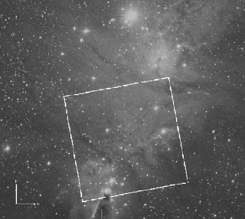
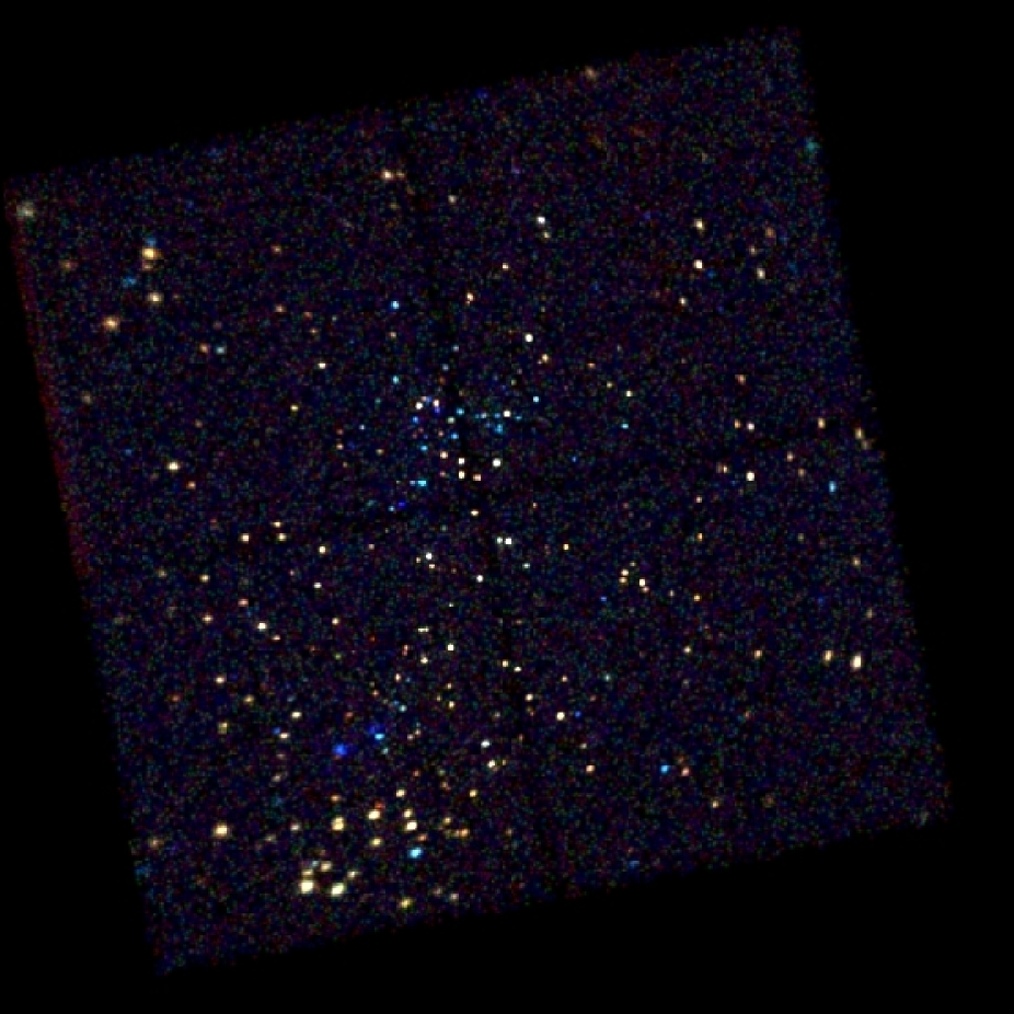
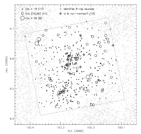
We obtained a 97 ks long ACIS-I exposure of NGC 2264 on 28 Oct. 2002 (Obs. Id. 2540; GO proposal PI S. Sciortino). The 17′17′field of view (FOV) of ACIS is shown in figure 1, superimposed on the Digitized Sky Survey image of the region. It was centered on R.A. 6h 40m 587, Dec. 9°34′14″(roll angle: 79°). Figure 2 shows a color rendition of the spatial and spectral information we obtained. ACIS was operated in FAINT mode with CCD 0, 1, 2, 3, 6 and 7 turned on. Data obtained with CCD 6 and 7, part of the ACIS-S array, will not be discussed in the following because of the much degraded point spread function (PSF) and effective area resulting from their large distance from the optical axis.
2.2 Data preparation
Data reduction, starting from the level 1 event file, was performed in a standard fashion, using the CIAO 2.3 package and following the threads provided by the Chandra X-ray Center111see cxc.harvard.edu. Several IDL custom programs were also employed. First, we corrected the degradation in the spectral response due to the Charge Transfer Inefficiency (CTI), occurred in particular during the first months of the Chandra mission using the acis_process_events CIAO task. We then produced a level 2 event file by retaining only events with grade=0,2,3,4,6 and status=0. Finally we corrected the data for the time dependence of the energy gain using the corr_tgain utility.
X-ray stellar sources have, on average, a different spectrum with respect to the ACIS background. The total signal to noise ratio (SNR) of sources can therefore be maximized by filtering out events with energy outside a suitable spectral band: we first performed a preliminary source detection as discussed in §2.3 on the whole event list. We then defined for each source a radius, , such that 97% of the PSF counts fall within this radius (§2.4). We extracted source photons for all sources from circles with and background photons from a single background region that excludes photons from all sources within their respective (a sort of “Swiss cheese” image with the sources carved out). We then computed the total SNR of sources222 where ; and are the number of counts in the -th source regions and their area respectively. and are the background counts and relative extraction area, taken for the present purpose as uniform within the FOV. for a fine grid of minimum and maximum energy cuts. The highest source SNR was obtained for and . With these cuts the number of photons in the source extraction area (including background photons) is reduced to 96% of the total, while the background is reduced to 28% of the total. We checked that consistent results are obtained by maximizing the SNR of faint sources only (20 net counts), which may have a different average spectrum and are the ones we are most interested in for the purpose of detection.
After filtering in energy, the time integrated background is 0.07 counts per arcsec2, consistent with nominal values. The background was constant in time except for a small flare with a peak reaching about twice the quiescent rate. The flare starts 13 ks after the beginning of the observation and lasts ks. The effect of the background flare on source light curves is however negligible, even for faint sources, i.e. the most affected by the background. This is confirmed by the negative results of Kolmogorov-Smirnov variability tests (see §4.1) performed on the background extraction regions relative to each source. In the study of source lightcurves (§4.1) we will therefore assume a constant background.
2.3 Source detection
We detected sources using the PWDetect code
(Damiani et al., 1997).333Available at:
http://www.astropa.unipa.it/progetti_ricerca/PWDetect The
significance threshold was set to 4.6. According to extensive
simulations of source-free fields with the background level of our
observation, this threshold corresponds to an expectancy of 10 spurious
sources in the whole FOV. PWDetect reports 423 sources. Upon careful
inspection we removed three entries relative to sources that were
detected twice, leaving a total of 420 distinct sources. Twenty eight
of these are below the 5.0 significance threshold,
corresponding to the more conservative criteria of one expected
spurious source in the FOV. Background subtracted source counts, in the
0.2-7 keV band, are derived by PWDetect directly from the wavelet
transform of the data. Effective exposure times at the source
positions, averaged over the PSF, are also computed by PWdetect from an
exposure map created with standard CIAO tools assuming an input energy
of 2.0 keV444The choice of energy is not crucial: the ratio
between the effective area at the source position and on the optical
axis, which is the quantity we use to define the effective exposure
time, has only a small dependence on energy..
Detected sources are listed in Table 1. In the first eight columns we report source number, sky positions with uncertainty, distance from the Chandra optical axis, source net counts (in the 0.2-7keV band), effective exposure time, and the statistical significance of the detection.
| N | RA | Dec. | Offax | Net Cts. | Exp. T. | Signif | (Ref) | Mod | [u] | |||
|---|---|---|---|---|---|---|---|---|---|---|---|---|
| [h m s] | [d m s]. | [”] | [’] | [s] | [cm-2] | [] | ||||||
| 1 | 6:40:25.8 | 9:29:24.0 | 3.14 | 9.5 | 25.1 | 80579 | 6.1 | 0.088 | 1.59 | JHK | – | -14.03 |
| 2 | 6:40:27.7 | 9:32:00.1 | 1.52 | 8.0 | 81.2 | 82888 | 16.2 | 0.262 | 0.00 | Av | 1T | -14.35 |
| 3 | 6:40:28.1 | 9:35:33.7 | 1.37 | 7.7 | 44.7 | 81810 | 9.0 | 0.032 | 0.00 | Av | – | -14.52 |
| 4 | 6:40:28.6 | 9:35:47.3 | 1.22 | 7.6 | 186.6 | 64151 | 29.6 | 0.000 | 0.10 | Av | 1T | -13.69 |
| 5 | 6:40:28.8 | 9:30:59.6 | 0.59 | 8.1 | 1222.2 | 82889 | 70.2 | 0.000 | 0.26 | Av | 2T | -12.74 |
| 6 | 6:40:28.8 | 9:33:05.3 | 0.80 | 7.5 | 111.0 | 83404 | 17.7 | 0.579 | 0.00 | Av | 1T | -14.12 |
| 7 | 6:40:30.6 | 9:38:37.7 | 1.84 | 8.2 | 11.1 | 82255 | 4.7 | 0.724 | – | – | – | – |
| 8 | 6:40:30.9 | 9:34:40.4 | 0.92 | 6.9 | 179.1 | 83958 | 25.7 | 0.001 | 0.62 | X | 1T | -13.48 |
| 9 | 6:40:31.2 | 9:31:07.0 | 0.71 | 7.5 | 506.4 | 84042 | 45.7 | 0.093 | 0.09 | Av | 2T | -13.31 |
| 10 | 6:40:31.7 | 9:33:28.9 | 1.64 | 6.7 | 18.9 | 84683 | 6.0 | 0.045 | 0.00 | JHK | – | -14.91 |
First 10 rows. The entire table, containing 420 entries, is available in the electronic edition of A&A.
2.4 Photon Extraction
Source and background photon extraction for spectral and timing analysis was performed using CIAO and custom IDL software. We first determined for each source the expected PSF using the CIAO mkpsf tool, assuming a monochromatic source spectrum (E=1.5 keV). We thus determined the expected encircled energy fraction as a function of distance from the source. Photons extraction circles were defined so as to contain 90% of the PSF, save for 28 sources for which the encircled PSF fractions were reduced to values ranging from 74% to 89% to avoid overlap with neighboring sources. The local background for each source was determined from annuli whose inner radii excludes 97% of the PSF and with outer radii twice as large. In order to exclude contamination of the background regions from the emission of neighboring sources we excluded from these annuli photons falling within the 97% encircled counts radii of all sources. The area of background extraction regions were computed through a mask in which we drilled regions outside the detector boundaries and circles containing 97% of the PSF photons from all sources.
For sources with at least 50 photons, source and background spectra suited to the XSPEC spectral fitting package were then created using standard CIAO tools. Corresponding response matrices and effective areas (RMF and ARF files respectively) were also produced with CIAO. For spectral analysis, spectra were energy binned so that each bin contains a fixed number of photons, depending on net source counts : 15 photons per bin for , 10 photons for and 5 photons for . Because spectral analysis (§4.2) was restricted to energies keV, the first energy bin was forced to begin at that energy.
3 Ancillary data
3.1 Cross-identifications - optical/NIR catalogs
We have cross-identified our X-ray source list with catalogs from the following optical/NIR surveys covering the whole area of our ACIS field: 2Mass (NIR photometry), Walker (1956, optical photometry + spectroscopy), Rebull et al. (2002, optical/NIR photometry + low resolution optical spectroscopy)555The Rebull et al. (2002), catalog was updated following private communication from L. Rebull, Lamm et al. (2004, optical photometry + variability), Dahm & Simon (2005, optical photometry + spectroscopy), Flaccomio et al. (2000, X-ray sources). The seven cross-identified catalogs are listed in the first column of table 2. In the 2nd column we indicate the number of objects within the ACIS FOV and in the third the number of objects identified with ACIS sources and of those for which the identification is unique. Adopted positional tolerances for cross-identifications are reported in the 4th column, either as a single figure for the whole catalog or as a range when defined for each individual object (see the table footnotes). They are based on the uncertainties quoted for each catalog.
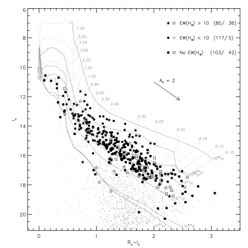
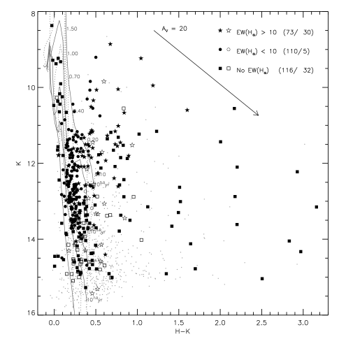
Among the catalogs here considered, the deepest photometric surveys are 2Mass in the NIR (JHKs666Note that in the following we neglect the small differences among NIR photometric systems, and in particular that between the 2MASS Ks and the standard K bands.) and Lamm et al. (2004) in the optical (V). A comparison with the isochrones of Siess et al. (2000, hereafter, SDF) in the optical and NIR color-magnitude diagrams (Fig. 3 and 4), indicates that at the distance of NGC 2264, 2Mass reaches down to about 0.1 for 10Myr old stars, i.e. the oldest expected in the region, while Lamm et al. (2004) reaches slightly deeper for unabsorbed stars, but is obviously less sensitive to highly absorbed ones. Within the ACIS FOV, spectral types are given for 7 stars by Walker (1956), for 87 stars by Rebull et al. (2002), for 150 stars by Lamm et al. (2004) and for 157 stars by Dahm & Simon (2005).
| Catalog | Id.Rad. | R.A. | Dec. | |||
|---|---|---|---|---|---|---|
| [″] | [″] | [″] | [″] | |||
| ACIS | 420 | — | 1.0-12.6a | -0.09 | -0.09 | 0.24 |
| 2Mass | 1098 | 346/344 | 0.5-1.4b | 0.00 | 0.00 | – |
| Walker (1956) | 67 | 52/52 | 1.0 | -0.45 | 0.08 | 0.47 |
| Rebull et al. (2002) | 511 | 236/235 | 1.5 | 0.73 | -0.03 | 0.73 |
| Lamm et al. (2004) | 1598 | 305/299 | 1.0 | -0.13 | 0.45 | 0.47 |
| Dahm & Simon (2005) | 229 | 183/183 | 1.0 | -0.16 | 0.18 | 0.36 |
| Flaccomio et al. (2000) | 84 | 80/80 | 8.1-42.8c | -0.85 | 1.49 | 3.70 |
a . Mean/median: 1.74″/1.25″
b .
Mean/median: 0.54″/0.50″
c 85% point source encircled energy radii (Flaccomio et al., 2000).
Mean/median: 12.0″/9.2″.
We created a master list of cross-identified objects following a step-by-step procedure. In the first step we matched ACIS sources with 2Mass objects: first we registered the ACIS coordinates to the 2Mass ones by iteratively cross-identifying the two catalogs and shifting the ACIS coordinates by the mean offset of uniquely identified source pairs. Identification radii were chosen as the quadrature sum of the above defined position tolerances (table 2). We then created a joint catalog of objects containing all matched and unmatched ACIS and 2Mass objects, assigning to them coordinated from 2MASS when available. In the following step we repeated the above process using the ACIS+2Mass catalog as reference and matching it with the Rebull et al. (2002) one. We then repeated the process with the Flaccomio et al. (2000) X-ray source list, then with the Lamm et al. (2004), Dahm & Simon (2005) and Walker (1956) catalogs. The coordinate shifts of all considered catalogs with respect to the 2Mass system are given in table 2 (columns 5 and 6), along with the median offsets between object positions and the reference 2Mass catalog. After each step, identified source pairs and unidentified objects were checked individually and a small fractions of the identifications () were modified. In the first step for example, five identifications between four ACIS and five 2Mass sources were added: in two cases (sources #64 and #404) 2Mass sources were only slightly more distant with respect to the identification radii. In another case the X-ray source, #102, was situated at the edge of the detector and its positions was surely more uncertain than the formal error indicated. In the last case the X-ray source, #237, was detected between two close-by 2Mass objects and an identification was forced with both.
Table 3 lists, for the 1888 distinct objects in the ACIS FOV, consolidated coordinates and cross-identifications numbers for each of the seven catalogs. 425 rows refer to objects related to one of the 420 ACIS sources: 351 are identified with a single optical/NIR counterpart, two are identified with 5 and 2 counterparts respectively, and 67 do not have any optical or near-infrared identification. The other 1463 rows in table 3 refer to non ACIS-detected objects. For these latter we computed upper limits to the ACIS count rate using PWdetect and the same event file used for source detection. Measured count rates, repeated from table 1, and upper limits are reported in column 12 of table 3.
Focusing on the identification of ACIS sources with optical/NIR catalogs, given the relatively large number objects in the field of view, we can wonder how many of the identifications are due to chance alignment and not to a true physical association. We can constrain the number of chance identifications by assuming that positions in the two lists are fully uncorrelated. Because this is surely not the case for our full X-ray source catalog, our estimate can only be considered a loose upper limit. Furthermore, limiting our X-ray sample to the 28 sources with significance below 5.0, 9 of which are expected to be spurious and whose positions will indeed be random, we can place an upper limit on the fraction of spurious sources associated with an optical object. This value is of interest when studying the X-ray properties of optically/NIR selected samples. In order to estimate the number of spurious identifications assuming uncorrelated positions, we proceed as follows: for each X-ray source we consider optical objects within a circular neighborhood of area , within which source density is assumed uniform; we then estimate the fraction of covered by identification circles. The sum of these fractions is our upper limit to the number of chance identifications. We repeated the calculation for radii of the neighborhood circle from 1.0′ to 4.0′. The upper limit to the number of chance identifications for the full sample of ACIS sources ranges from 13 to 15. For the 28 source with significance we instead estimate no more than 2.5 chance identifications. If we assume that out of the 28 sources, only the nine spurious detections have positions that are indeed uncorrelated with optical objects, we can scale this result and conclude that spurious X-ray source will be by chance identified with an optical object. Conversely, we can most likely locate spurious sources among the 15 sources with significance below 5.0 and that are not identified with optical/NIR catalogs.
| N | RA | Dec. | Id. rad. | ACIS | 2Mass | Reb.+ | Lamm+ | Flacc+ | W56 | Dahm+ | Ct. Rate. |
|---|---|---|---|---|---|---|---|---|---|---|---|
| [h m s] | [d m s] | [”] | [ | ||||||||
| 1 | 6:40:22.4 | 9:28:03.2 | 0.54 | – | 06402243+0928032 | – | 3228 | – | – | – | 8.7 |
| 2 | 6:40:24.2 | 9:30:38.1 | 0.50 | – | 06402419+0930381 | 2229 | – | – | – | – | 3.3 |
| 3 | 6:40:24.3 | 9:27:44.4 | 0.50 | – | 06402425+0927443 | – | – | – | – | – | 23.5 |
| 4 | 6:40:24.8 | 9:29:39.6 | 0.66 | – | 06402475+0929395 | – | – | – | – | – | 3.4 |
| 5 | 6:40:24.8 | 9:28:42.6 | 0.50 | – | 06402482+0928425 | – | – | – | – | – | 3.3 |
| 6 | 6:40:24.8 | 9:28:59.8 | 0.64 | – | 06402482+0928597 | – | – | – | – | – | 3.5 |
| 7 | 6:40:25.0 | 9:30:00.5 | 1.00 | – | – | – | 3295 | – | – | – | 3.0 |
| 8* | 6:40:25.0 | 9:32:08.4 | 0.50 | – | 06402504+0932084 | 2258 | 3299 | – | – | – | 4.1 |
| 9 | 6:40:25.1 | 9:29:36.9 | 0.50 | – | 06402505+0929369 | 2261 | 3300 | – | – | – | 3.4 |
| 10 | 6:40:25.4 | 9:30:26.4 | 1.00 | – | – | – | 3326 | – | – | – | 2.8 |
*: Likely NGC 2264 member;
†: Entry also present in another row.
First 10 rows. The entire table, containing 1888 entries, is available in the electronic edition of A&A.
3.2 Characterization of stars in the FOV
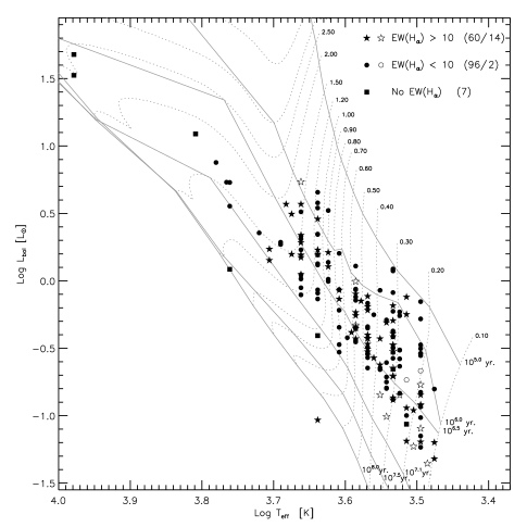
We have collected optical and NIR data from the literature for all the stars in the master catalog assembled in the previous section. In table 4 we report photometry and spectral types for our X-ray sources with unique optical identification. A total of 300 X-ray detected stars have been assigned both and magnitudes and are plotted in figure 3 as filled symbols; 299 have H and K magnitudes and are plotted in figure 4 (264 of these also appear in Fig. 3). In both color magnitude diagrams (CMDs) we also show for reference SDF tracks and isochrones, transformed to colors and magnitudes using the conversion table given by Kenyon & Hartmann (1995) and shifted along the reddening vectors by the median extinction of known members () and vertically by the distance modulus corresponding to the adopted distance. For the extinction law we adopted Rieke & Lebofsky (1985). For stars with spectral types we derived effective temperatures, , bolometric corrections, , and intrinsic colors, , using the relations compiled by Kenyon & Hartmann (1995) and, for the temperature of M stars, the intermediate gravity scale of Luhman (1999). Using the available and photometry we then derived extinction values (, where ) and bolometric luminosities (]). Finally we estimated masses and ages from the theoretical HR diagram, figure 5, through interpolation of the SDF evolutionary tracks. In summary, out of the 351 X-ray sources with an unique optical/NIR identification, we estimated for 165 X-ray sources, and for 163, masses and ages for 161.
Other than the sample of X-ray detected stars, that, as discussed in §5 are likely cluster members, we will also consider another sample of 83 X-ray undetected likely cluster members. These latter, plotted with empty symbols in figure 3, 4 and 5, are chosen according to their position in the I vs. R-I diagram, the strength of the line (measured either spectroscopically or photometrically) and optical variability: first, we define a cluster locus in the I vs. R-I diagram using the SDF tracks and the observed concentration of X-ray sources. The cluster locus is defined as the area above the Myr isochrone or to the left of the 0.8 evolutionary track.777This latter condition is required by the convergence of the isochrones at higher masses and by the observed spread of stars in the “cluster locus”, at least in part due to uncertainties. We then consider as likely members: stars in the cluster locus and with strong emission according to the narrow-band photometry of Lamm et al. (2004), using the same criterion discussed by these authors; stars in the cluster locus with moderate (chromospheric) emission and with variable optical lightcurves (both periodic and irregular), again as discussed by Lamm et al. (2004); stars for which spectroscopic observations of the line are available and for which the measured EW is larger than 10 (the canonical CTTS threshold). Among this sample of 83 X-ray undetected likely members we are able to determine masses and ages for 16 stars.
| N | R | R-I | J | H | K | Sp.T. | Av | Av(JHK) | Mass | LogAge | |||
|---|---|---|---|---|---|---|---|---|---|---|---|---|---|
| [K] | [] | [] | [yr.] | [d] | |||||||||
| 1 | 17.97 | 2.10 | 15.92 | 14.17 | 13.37 | – | – | 9.96 | – | – | – | – | – |
| 2 | 15.68 | 1.25 | 14.27 | 13.54 | 13.29 | M2.5 | 0.00 | 0.62 | 3.54 | -0.80 | 0.34 | 6.63 | 1.23 |
| 3 | 15.88 | 1.33 | 14.44 | 13.70 | 13.50 | M3 | 0.00 | 0.00 | 3.53 | -0.87 | 0.30 | 6.63 | 12.09 |
| 4 | 14.14 | 1.03 | 12.79 | 12.07 | 11.85 | M0 | 0.62 | 0.41 | 3.59 | -0.06 | 0.57 | 6.11 | 4.55 |
| 5 | 13.26 | 0.86 | 11.81 | 11.30 | 10.75 | K4 | 1.61 | 0.00 | 3.66 | 0.51 | 1.57 | 6.19 | 7.49 |
| 6 | 15.15 | 1.33 | 13.66 | 12.97 | 12.78 | M3 | 0.00 | 0.00 | 3.53 | -0.57 | 0.32 | 6.33 | 0.76 |
| 7 | 19.86 | 1.74 | – | – | – | – | – | – | – | – | – | – | – |
| 8 | 14.39 | 0.86 | 12.69 | 11.51 | 10.67 | K1 | 1.92 | 2.39 | 3.71 | 0.15 | 1.30 | 7.10 | 12.09 |
| 9 | 13.82 | 0.83 | 12.57 | 11.90 | 11.62 | K6 | 0.58 | 0.00 | 3.62 | 0.01 | 0.92 | 6.38 | 1.98 |
| 10 | 17.06 | 1.70 | 15.42 | 14.85 | 14.60 | – | – | 0.00 | – | – | – | – | – |
First 10 rows. The entire table, containing 420 entries, is available in the electronic edition of A&A.
In order to derive intrinsic X-ray luminosities of detected stars or upper limits for undetected ones, knowledge of the extinction is fundamental (§4.3). For stars with no optical spectral type cannot be determined as indicated above. We therefore estimated extinctions from the NIR J-H vs. H-K diagram by de-reddening stars that could be placed in this diagram onto the expected intrinsic locus. This latter was taken from Kenyon & Hartmann (1995) for the stellar contribution and supplemented with the CTTS locus of Meyer et al. (1997). The degeneracy in the reddening solutions was solved by always taking the first intercept between the intrinsic locus and the reddening vector. Stars whose position was within 1.5 of the loci were assigned zero extinction. In summary, we obtained a total of 278 and 62 extinction values for X-ray detected stars and undetected likely members, respectively. These number exceed by 115 and 46 the number of extinctions derived from optical data for the same samples. Although these NIR extinction values are surely more uncertain than the ones derived from spectral types, they are especially valuable for highly extinct objects.
3.3 Cross-identifications - MIR/mm catalogs
In addition to the wide field surveys described in §3.1 we have also correlated our X-ray sources with three mid-infrared (MIR) and millimeter (mm) catalogs recently published for the IRS 2 and IRS 1 regions: Young et al. (2006, hereafter Y06), Teixeira et al. (2006, T06) and Peretto et al. (2006, P06). These three surveys target very young and/or embedded objects and are therefore ideal for checking the nature of X-ray sources with no optical/NIR counterpart. They are however limited in area coverage: T06 lists Class I/0 sources detected with SPITZER in a arcmin2 region close to IRS 2; Y06 lists all SPITZER detected objects in a dense but even smaller arcmin2 region slightly south-east of IRS 2; P06 list the pre/protostellar cores detected at 1.2mm in both the IRS 1 and IRS 2 regions.
Within the area of Y06, the only MIR work available so far that lists all the objects detected in the surveyed region, we find MIR counterparts for 2 out of 4 X-ray sources lacking optical/NIR counterparts. In total 4 of the 67 unidentified X-ray sources were assigned new counterparts: #145 was associated with source 12 of T06, a Class I/0 source; #228 was associated with the D-MM 15 mm core, indicated by P06 as probably starless; #244 was associated with source 43 in Y06 and is, judging from its spectral energy distribution (SED), an absorbed class II/III PMS star that is relatively bright in -band (, Y06)888Note that the source is missed by 2MASS because, at the 2MASS spatial resolution, it is blended with a nearby source; finally #274 was associated with the D-MM 10 mm core, indicated as starless by P06, with source 1656 in Y06 and source 15 in T06 (characterized by a steeply rising MIR SED).
Among the X-ray sources with optical/NIR counterparts, 17 in the region covered by Y06 were identified with SPITZER sources of which one, #281, is a likely Class I source (Y06’s source 62). Three more X-ray sources were identified with Class I/0 sources in the list of T06: #150 and #242 also having NIR counterparts and #194 (see also §6.3) with both NIR and optical () counterpart. As for the P06 mm-cores, identifications are made uncertain by the limited spatial resolution of the mm data (cf. P06). The core D-MM 14, classified as protostellar by P06, is likely associated with ACIS source #89 (offset: 1.2”), an optically faint () and NIR bright () star with large emission: . Quite similarly, C-MM 1, also indicated as a protostellar core by P06, is offset by 1.3” from the ACIS source #361, an optically visible source with strong (, , )999Although Y06 report that C-MM 1 has no NIR counterpart, we associate it with 2MASS source 06411792+0929011 (offset=1.5”). and it is therefore likely associated with it. Finally, C-MM 5, classified by P06 as a protostellar core, might be associated with ACIS # 305 (offset: 1.9”). This ACIS source is in turn most likely associated with IRS 1 (offset: 0.8”, Schreyer et al., 2003). Note however that P06 suggests that C-MM 5 may not be associated with IRS 1.
A more detailed analysis of the X-ray properties of young protostars in NGC 2264 will be the subject of a future paper.
4 Analysis
4.1 Temporal analysis
Source variability was characterized through the Kolmogorov-Smirnov test. Column (9) of table 1 reports the resulting probability that the distribution of photon arrival times is not compatible with a constant count-rate. Given the sample size (420 sources) a value below 0.1% (obtained for 72 sources) indicates the light-curve is almost certainly variable, while a 1% value (87 sources) indicates a very likely variability, although up to of the variable sources might actually be constant. If we are not interested in the individual sources but on the overall fraction of variable sources, we can place a lower limit on this quantity by computing the minimum number of variable sources as a function of probability threshold, : . The maximum is obtained for % for which and . We conclude that within our observation at least 30% (126/420) of the lightcurves are statistically inconsistent with constancy. This fraction is surely a lower limit to the true number of variable sources, as our ability to tell a variable source from a constant one is influenced by photon statistics. This is clearly indicated by the dependence of the fraction of variable sources on source counts. If for example, we restrict the above analysis to sources with more than 100(500) counts, a total of 145(33) sources, we find that at least 54%(73%) of these are variable.
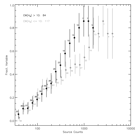
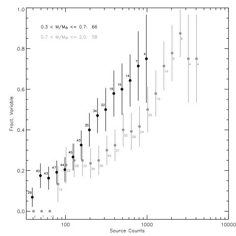
We next investigated whether different kind of stars, classified from optical data, showed different variability fractions. From the previous discussion, it is clear that for a meaningful comparison, source statistic must be taken into account. Figure 6 shows the variability fraction, , as a function of source counts for CTTS and WTTS, as discriminated by their equivalent width. Variability fractions are computed for sources with counts in intervals spanning 0.8 dex (because in the figure points are spaced by 0.1 dex, only one point every eighth is independent). Error bars on the variability fractions are estimated assuming binomial statistics: , where is the number of sources in each count bin. In addition to the expected increase of the variability fraction with source statistics, we note that CTTS appear to be more variable with respect to WTTS, at least when considering stars with more than 200 counts. Figure 7 shows a similar comparison for two mass segregated sub-samples: and . Lower mass stars appear to be more variable, and again this difference is noticeable only for stars that are bright enough. We quantified the differences between variability fractions, by testing, for each count bin, the null hypothesis that the two samples are drawn from the same parent population. We chose as statistics the difference of the two observed variability fractions, . We then numerically computed the probability that a equal or larger than the observed one is obtained by randomly drawing pairs of numbers from binomial distributions appropriate to the two sample sizes but characterized by the same probability of observing a variable source, i.e the variability fraction. Because this latter number is not well constrained we conservatively took as our confidence level the minimum that is obtained varying this fraction between 0 and 1. The results of these test indicate that the differences in the variability fractions are statistically not highly significant: in the bin centered at counts, the low mass stars are more variable than higher mass stars with a 94% confidence. In the bin centered at counts, CTTS are more variable than WTTS with a 92% confidence. We thus consider these results as tentative. However we note that the significance of the difference between CTTS and WTTS is strengthened by the fact that a similar result, and with a similar confidence, was also obtained by Flaccomio et al. (2000) using totally independent ROSAT data.
4.2 Spectral analysis
We have analyzed the X-ray spectra of the 199 sources with more than 50 detected photons. Spectral fits were performed with XSPEC 11.3 and several shell and TCL scripts to automate the process. For each source we fit the data in the [0.5-7.0]keV energy interval101010 Events with energies below 0.5keV were not used because of uncertainties in the calibration resulting from the time dependent degradation of the ACIS quantum efficiency at low energies. with several model spectra: one and two isothermal components (apec), subject to photoelectric absorption from interstellar and circumstellar material (wabs). Plasma abundances for one temperature models were fixed at 0.3 times the solar abundances (Wilms et al., 2000), while for two temperature models they were both fixed at that value and treated as a free parameter. The absorbing column densities, , were both left as a free parameter and fixed at values corresponding to the optically/NIR determined extinctions, when available: (Vuong et al., 2003). A total of three or six models were thus fit for each source depending on the availability of optical extinction values. For each model, spectral fits were performed starting from several initial conditions for the fit parameters as indicated in table 5. For example for isothermal models with free , two values of and four values of were adopted as initial conditions, for a total of eight distinct fits. For each model the adopted fit parameter set was chosen from the model fit that minimize the . This procedure was adopted in order to reduce the risk that the minimization algorithm used by XSPEC finds a relative minimum.
| Model name | [cm-2] | Abund. | |
|---|---|---|---|
| 1T | 0.0, | 0.5/–, 1.0/–, 2.0/–, 10.0/– | 0.3 |
| 2T | 0.0, | 0.4/1.0, 1.0/3.0, 0.5/2.0 | 0.3 |
| 2Tab | 0.0, | 0.4/1.0, 1.0/3.0, 0.5/2.0 | 0.3 |
| 1TAv | 1.610 | 0.5/–, 1.0/–, 2.0/–, 10.0/– | 0.3 |
| 2TAv | 1.610 | 0.4/1.0, 1.0/3.0, 0.5/2.0 | 0.3 |
| 2TabAv | 1.610 | 0.4/1.0, 1.0/3.0, 0.5/2.0 | 0.3 |
Multiple values indicate that all combinations of initial values were adopted. Values in italic indicate that fit parameters were fixed to those values.
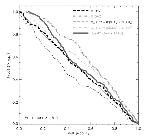
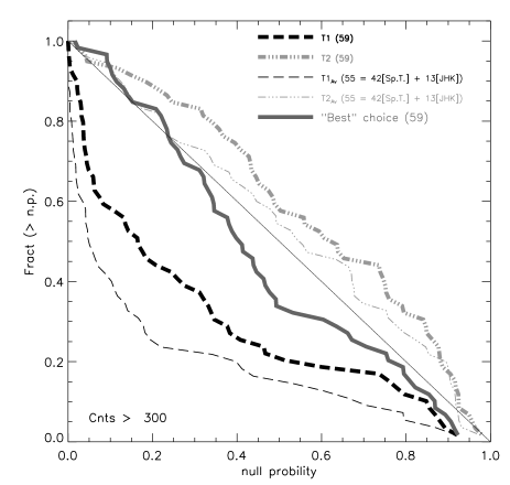
Next, we considered which of the available model fits for each source (three or six, reference model names are given in table 5) was the most representative of the true source spectra, and thus the one to be adopted for the following considerations. The goal was twofold: to characterize the emitting plasma in order to investigate its origin, and to determine accurate intrinsic band-integrated X-ray luminosities. Crucial for this latter step is the determination of extinction (, see §4.3). Generally speaking, models must have enough components to yield statistically acceptable fits according to the or, equivalently, the null probabilities (n.p.) that the observed spectra are described by the models. However, models with too many free parameters with respect to the spectra statistics, while formally yielding good fits, will not be constrained by the data and will yield limited physical information. A particularly severe problem with CCD quality (ACIS) low statistic spectra is the degeneracy between absorption and temperature: an equally good fit can be often obtained with a cool plasma model with a large emission measure but suffering high absorption, or with a warmer temperature and a lower extinction. It is therefore desirable to check the obtained from the fits with independent information from optical/NIR data. Figures 8 and 9 show, for faint and bright sources (, ) respectively, the cumulative distribution of the n.p. for spectral fits performed with four different models. The models are 1T, 2T, and, for sources with independent estimates, 1TAv and 2TAv. In this kind of plot the distribution for a perfectly adequate spectral model should follow the diagonal, that for an oversimplified model should fall below the diagonal, and that for an over-specified model should lie above. For faint sources 1T model appears perfectly adequate. Fixing the to the optically determined value worsen the agreement somewhat but still results in fits that are, when considered individually, for the most part acceptable. A two temperature model with free appears to be too complicated (and therefore unconstrained), while a 2T model with fixed is more acceptable, but still on average too sophisticated for the quality of these low-statistic spectra. For brighter sources we notice instead that 1 temperature models are on average not favored, while 2T models are still not always needed.
For most sources more than one spectral model is statistically acceptable. We choose a best guess model as the simplest that still gives a statistically acceptable fit. The compelling reason to choose this approach is the mentioned degeneracy between temperature and absorption. Note for example that from figure 8, one could be tempted to always choose, for faint sources, 1T models with free , as these models appear to be statistically perfectly adequate to represent the spectra. However, when examined individually, many of these 1T spectral fits have rather degenerate fit solutions, i.e. large and correlated uncertainties on the and values, also implying large uncertainties on unabsorbed fluxes. This degeneracy can be broken by using the additional information on absorption coming from optical/NIR data, when available and compatible with the X-ray spectra.
After some experimenting, we choose our best guess model according to the following empirical scheme: if n.p.(1T we chose the 1TAv model. Otherwise, if n.p.(1T) we chose the 1T model (with free ). If both of the previous tests for isothermal models failed, we tried with two temperature models, this time lowering our n.p. threshold to 5%. First we tried the 2TAv model (n.p.(2T) and then the 2T model (n.p.(2T)). As a last resort, in case none of the previous models could be adopted, we choose the 2Tab model (free , free abundances). Although the above scheme was designed so to favor simple models, the different n.p. thresholds resulted in four cases (sources #257, #275, #280 and #300) in adopting 2Tab models that were either statistically worse or comparable to simpler 1T, 1TAv or 2TabAv models. We therefore adopted these latter. After careful examination of individual fits, the spectral models adopted for four more sources (#97, #104, #127 and #241) were modified. In these cases the automatic choice would result in unphysical, unusual, or unconstrained temperatures and absorptions, whereas our adopted models are acceptable both statistically and physically.111111For source #241 we changed the 2T model (n.p.=32%, keV, keV, ) to a 1T model (n.p.=17%, keV, ). For source #104 we changed the 1T model (n.p.=40%, keV, ) to a model (n.p.=32%, and reasonable temperatures). For sources #97 and #127 we changed from models (p=68% & p=0.21%, keV & keV, both with unconstrained uncertainties) to 1T models (p=97% & p=56%, keV & keV).
The solid gray lines in figure 8 and 9 refer to the final choice of best guess models. Table 6 lists the end result of our spectral analysis: we report the adopted model, the source of the adopted , the null probability, the plasma temperature(s) and normalization(s), the observed and absorption corrected fluxes in the [0.5-7]keV band.
| N | Mod | (Ref) | [a] | [u] | ||||||
|---|---|---|---|---|---|---|---|---|---|---|
| [cm-2] | [keV] | [keV] | [] | [] | ||||||
| 2 | 1T | Av | 0.40 | -14.35 | -14.35 | |||||
| 4 | 1T | Av | 0.62 | -13.78 | -13.69 | |||||
| 5 | 2T | Av | 0.14 | -13.07 | -12.74 | |||||
| 6 | 1T | Av | 0.85 | -14.12 | -14.12 | |||||
| 8 | 1T | X | 0.41 | -13.62 | -13.48 | |||||
| 9 | 2T | Av | 0.92 | -13.43 | -13.31 | |||||
| 11 | 1T | JHK | 0.17 | -13.86 | -13.75 |
First 7 rows. The entire table, containing 199 entries, is available in the electronic edition of A&A.
In summary, out of the 199 sources with more than 50 counts, we adopt isothermal models in 147 cases and two component models in the remaining 52 cases. For 138 sources we adopt a spectral fit in which the was fixed, in 101 cases to the value estimated from the optically determined and in 37 cases from NIR photometry. In the remaining 61 cases was treated as a free fit parameter. Out of these 61 cases, independent estimates of extinction were available from optical and NIR data in 21 and 3 cases respectively, but our algorithm (or, for sources #97 and #127, our choice) preferred the spectral fit with free . We examine these cases more in detail to assess the ambiguities in the model fits and the consequences on the derived X-ray fluxes.
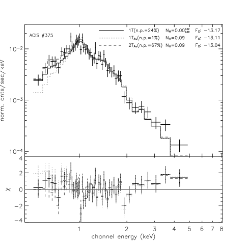
Figure 10 illustrates one of such cases: source #375. Here the extinction determined from the 1T (kT=1.3keV) spectral fit (90% confidence interval: cm-2) is lower than that estimated from the (cm-2). Fixing the to that value yields an unsatisfactory isothermal fit. We note however that adding to the spectral model a second cool isothermal component (kev), a good fit can be obtained even fixing the . This is a quite typical example of the degeneracy in the fitting of sources with low/moderate statistics. We can estimate the uncertainty in the X-ray unabsorbed fluxes derived from the spectral fits due to this degeneracy as the difference between the fluxes derived from the two acceptable fits: for source #375 for example this is dex. More in general, acceptable fits with fixed to the optical/NIR values could be obtains in 22 of the 24 cases in which our procedure preferred the spectral fit with free . In five cases121212Sources #190, #340, #352, #375, #391, among which that described above, in order to conciliate the observed spectra with the optical extinction, an additional cool thermal component (kT=0.22-0.34) would be required to compensate for the higher . If for these five sources the true were the optically derived ones, by choosing the 1T fit with free (lower) we are underestimating the unabsorbed fluxes by 0.14-0.37dex (mean 0.2dex). For the other 17 sources, fixing the would not require an additional component: reasonable fits (n.p. 5%) were obtained even with the same models (1T in 16 cases, 2Tab for source #187). In 10 of these 17 cases the adopted fits with free result in smaller absorptions and slightly hotter (0.2-0.3keV) temperatures (the cool temperature for #187), while the opposite happens in the other 7 cases. Had we fixed the to the optical values in these 17 cases we would have obtained unabsorbed fluxes on average 0.03dex larger and always within 0.20dex (in either direction) of the adopted ones.
From this discussion of the 22 cases with most ambiguous extinctions ( of the sources for which we have optical/NIR ), we conclude that: a) typical uncertainties in the unabsorbed flux are less than 0.2dex, b) individual X-ray fluxes corrected using an from spectral fits can be as wrong as 0.4 dex, if the cool temperature is altogether missed by the spectral fit with a consequent underestimation of the .
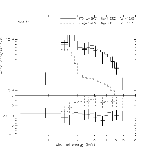
Two more sources have incompatible X-ray and optical extinctions according to our choice of best model. Source #234 did not enter in the previous discussion because it has the least acceptable fits of the whole sample, at most n.p. =1.6% for a 2T model with free (note, however, that with an adequate spectral model, we would expect three sources out of 199 to have lower n.p.). Adopting the optical () would result in an unabsorbed flux only 0.07dex larger with respect to that obtained leaving as a free fit parameter (). Source #71 is a more interesting case. Figure 11 shows its spectrum, with spectral fits obtained with free and fixed . The X-ray derived extinction () is about 17 times larger than that estimated from the optical reddening ()131313For this source we have adopted the spectral type (K2) from Dahm & Simon (2005) and the photometry () from Lamm et al. (2004). Independent photometry and spectral types are available from Rebull et al. (2002), Lamm et al. (2004) and Dahm & Simon (2005). ranges between 0.55 and 0.62 and spectral types between G9 and K2. The possible range in is thus , i.e. between and times the value derived from the X-ray spectrum, considering its 90% confidence interval.. The discrepancy is highly significant and independent of the considered spectral model. We note that the detected emission from this source is dominated by a powerful flare, with peak count rate 100 times that before and after the flare. A possible scenario to explain the high absorption might involve a solar-like coronal mass ejection associated with the flare, providing the additional absorbing material. Such an hypothesis has been formulated by Favata & Schmitt (1999) to explain a more modest increase in during a powerful flare observed on Algol.
Further discussion of physical interpretation of spectral fit results is deferred to §6.
4.3 X-ray luminosities
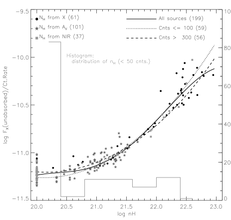
Extinction corrected X-ray luminosities in the [0.5-7.0]keV band were estimated for all sources for which an indication of extinction was available. For the 199 sources with more than 50 counts, and for which spectral fits were performed, we computed from the (unabsorbed fluxes) column in table 6, adopting a distance of 760pc, adequate for NGC 2264 members. For the fainter sources, for which spectral fits were not performed, we derived a count-rate to unabsorbed flux conversion factors using the results of the spectral fits for the brighter stars. Figure 12 shows, for these latter sample, the run of the flux/rate ratio vs. . Different symbols indicate different origins of the absorption values (see previous section). We then performed polynomial fits to the data points for the whole sample, for the 56 sources with more than 300 counts and for the 59 sources with less 100 counts. Results are shown in fig. 12. Because the sources for which we want to determine fluxes have 50 counts, we adopt the latter fit as our relation between and the conversion factor:
| (1) |
Where the units are ergs cm-2. The dispersion of the data-points around this relation is dex, which can be taken as an upper limit to the error on the source flux introduced by ignoring the spectral shape of faint sources. From the observed count-rates we thus estimated fluxes for 127 X-ray sources with 50 counts and with estimates coming from either the or the JHK photometry. The gray histogram in figure 12 shows the distribution of for these sources. Results are reported in table 1. Note that we do not quote X-ray fluxes for faint sources without an independent extinction estimate. Upper limit fluxes for 425 X-ray undetected stars in the ACIS FOV and with an absorption estimate (out of a total of 1463) were similarly computed from the upper-limits to the count rates.
5 Results - Membership
In this section we define a sample of 491 likely NGC 2264 members within the FOV of our ACIS observation. X-ray sources account for 408 objects while the remaining 83 are selected on the basis of the strength of line and of optical variability as described in §3.2. The likely members are indicated in table 3 by an asterisk following the identification number. We first consider the possibility of extragalactic contamination and then discuss separately the nature of X-ray sources with and without optical/NIR counterparts.
5.1 Extragalactic X-ray sources
Extragalactic contamination is expected only among X-ray sources that lack an optical and/or NIR counterpart. We reach this conclusion by considering the 489 ACIS sources of likely non stellar origin detected in the Chandra Deep Field North (CDFN; Alexander et al., 2003; Barger et al., 2003)141414We excluded 14 sources identified as stars by Barger et al. (2003).. After defining, for each CDFN source, random positions in our FOV, we compared their observed count rates with upper limits computed from our ACIS data at those positions (see §3.1). We then selected CDFN sources that would have been detected with our exposure: a total of objects151515Mean value and 1 uncertainty result from repeating the experiment 10 times, varying the position of simulated extragalactic sources.. Next, we compared the positions of these simulated CDFN AGNs in the optical (I vs. R-I) and NIR (H vs. H-K) color-magnitude diagrams161616The NIR photometry of the CDFN sources was taken from 2Mass. with those of the X-ray sources in the NGC 2264 exposure that could be placed in the same diagrams. These plots show that AGNs are on average considerably fainter than our identified X-ray sources that can be placed in either of these diagrams and only two or three of the AGNs that we could have detected occupy positions that overlap with the loci where our X-ray sources are found. We note moreover that in this comparison we have totally neglected the effect of extinction. Because of the dark cloud in our line of sight, the number of AGNs we are sensible to is surely much reduced with respect to the above estimate. Moreover the optical and NIR luminosities of AGNs would also be considerably reduced. We therefore conclude that the contamination of AGNs to the sample of X-ray selected likely members with optical/NIR identification is negligible.
5.2 X-ray sources with optical/NIR counterparts
In figure 3 we showed the optical CMD for the 300 X-ray sources that can be placed in such a diagram and for the 83 other undetected likely members discussed in §3.2. Note that the X-ray sources (filled symbols) are for the most part found in the locus expected for NGC 2264 members (i.e. the previously defined cluster locus). However some X-ray sources lie below that locus, their position being compatible with that expected for MS foreground stars. Very few, if any, of the X-ray sources in this diagram may be background MS stars, which are expected to lie below the 1Gyr isochrone. In order to reduce contamination in the sample of likely members to a minimum, we exclude X-ray sources that lie outside the cluster locus, i.e. below Myr isochrone and to the right of the 0.8 evolutionary track. We make an exception for two sources: #305 (I=17.28, R-I=0.98), associated with the IRAS source IRS-1, classified as a Class I object by Margulis et al. (1989) but more recently suggested to be a deeply embedded B star in a more evolved evolutionary stage (Schreyer et al., 2003)171717The ACIS spectrum indicates (90% confidence interval), corresponding to .; #309 (I=16.45, R-I=0.76), a known member, being indeed the peculiar and well studied accreting binary system KH 15D (e.g. Hamilton et al., 2005; Herbst & Moran, 2005; Dahm & Simon, 2005). The 8 sources that lie to the right of the 0.1 track are considered likely members, either of very low (sub)stellar mass or very absorbed. Lacking values from optical spectra, we can check these two possibilities using our X-ray data and the JHK photometry. Out of these 8 sources, 4 (#125, #192, #251, #273) are highly absorbed as indicated by their X-ray spectra (or hardness ratios) and/or their positions in the J-H vs. H-K diagram. Other three sources (#215, #316, #358) however appear to have negligible absorption and are good candidates for detected brown dwarfs.
Only 10 X-ray sources (out of 300) are excluded as members because incompatible with our cluster locus in the optical CMD and might be associated with field stars181818#7, #51, #110, #128, #130, #171, #224, #248, #258, and #267.. Among them only one (source #258, an X-ray faint and soft G5 star) could be placed in the HR diagram of figure 5, and is there placed on the 100Myr isochrone. Although we exclude these 10 sources from our sample of likely members, some of them might actually be members: i) in figure 3 six very likely members, 5 undetected and one detected CTTSs, are found below the cluster locus. This indicates that some members do have position in the optical CMD that differ from the expectations; ii) the spatial distribution of these 10 sources (figure 13, squares+dot symbols) is similar to that of cluster members, and not uniform as expected from foreground stars; iii) the ACIS spectra and hardness ratios indicate that 5 of these sources suffer high extinction in the X-ray band, which is incompatible with foreground MS star (but not with background giants).
We now statistically estimate the number of foreground stars that, present in our FOV and detected by ACIS, contaminate our list of 290 (=300-10) X-ray detected cluster-locus candidate members, as well as the 10 X-ray sources outside of the cluster locus. We considered the volume-limited stellar samples of the NEXXUS survey (Schmitt & Liefke, 2004), extracting from it a near-complete sample of stars of spectral types F to M within 6 pc from the Sun. These stars are optically well characterized and have known distances and X-ray luminosities as measured with ROSAT. We estimated the number of foreground stars, , in our FOV assuming that the spatial density of field stars in the direction of NGC 2264 is uniform and equal to that in the solar neighborhood191919This is justified by the low equatorial longitude of NGC 2264: .. We next randomly drew stars from the NEXXUS sample and assigned them random distances, , in the range [0-760]pc, according to an uniform stellar density. With these distances and assuming an isothermal X-ray spectrum with kT=0.3 keV, we converted the NEXXUS X-ray luminosities to ACIS count rates using an -dependent conversion factor calculated with the “Portable, Interactive Multi-Mission Simulator” (PIMMS). The hydrogen column density toward each star was estimated as , where the volume density was set to 0.3 and the distance is expressed in cm202020With the chosen value of , taking and d=760pc (the assumed distance of NGC 2264), we obtain =0.44, in agreement with the median of values measured for NGC 2264 members.. We finally compared these simulated count-rates with upper limits estimated at random positions in the ACIS FOV estimated using PWDetect (§3.1). This simulation was repeated 100 times, varying the sample of NEXXUS stars and their position in space. On average, the sample of foreground stars that we would have detected counts 20 stars, 15 of which should fall in the cluster locus and 5 outside of it. About half of the 10 stars outside the cluster locus are thus expected to be cluster members, thus reinforcing the arguments given in the previous paragraph. Within the cluster locus, only 5% (15/290) of the X-ray sources are estimated to be non-members212121The fraction of non-members is expected to be higher among X-ray sources with and ages yr.. Given that eighty of the X-ray sources in the cluster locus had not been previously selected as likely members because of either their emission or optical variability, we estimate that our sample contains new optically visible members.
Fifty-one more X-ray sources were identified with optical or NIR objects but could not be placed in the optical CMD (14 have I magnitudes but no R, 37 are only detected in 2MASS). Extending the previous result and because we can exclude an extragalactic nature for these sources, we consider these stars as additional candidate members. Only four of them had previous indication of membership from or optical variability.
5.3 Sources with no optical/NIR counterpart
Sixty-seven ACIS sources are not identified with any object listed in the full-field optical/NIR catalogs we have considered222222Four of these X-ray sources were actually identified with MIR and/or mm sources in §3.3. Because these catalogs are not spatially complete, for uniformity we here treat them as unidentified.. None of them was detected by Flaccomio et al. (2000) with the ROSAT HRI232323In table 3, due to the large uncertainty of the HRI positions, our ACIS source # 376 is associated with HRI source 138; the HRI source is however closer to the brighter ACIS source #375, with which it is most likely associated.. With respect to identified sources, they have significantly fewer counts. Fifteen non identified sources have detection significance and the 10 expected spurious detections (cf. §2.3) will be most likely found in this group. Nine have more than 50 counts and were subject to spectral analysis.
As discussed in §5.1, depending on the optical depth of the background cloud, a number of AGNs are expected to be detected in our FOV and will be found among the non-identified sources. It is therefore reasonable to ask whether the characteristics of our sources without counterparts are compatible with an AGN nature. The X-ray spectra of AGNs should be rather hard and well fit by power law models with indexes between 0.9 and 1.924242480% interval of the power indexes reported by Alexander et al. (2003) for the sources in the CDFN that we would have detected in our ACIS data and for which the 1 uncertainty in the index is lower than 0.1.. Their lightcurves should be constant or slowly varying. They should be distributed uniformly in space, or anti-correlated with the cloud optical depth. With respect to this latter point, figure 13 shows the spatial distribution of several classes of objects: circles of three different sizes indicate X-ray sources without counterparts in three source count ranges. Other X-ray sources are shown with black dots, while all the other objects in our master catalog are shown in gray. These latter are for the most part background field stars and their density is a good indicator of the optical depth of the molecular cloud. Note how the X-ray sources with counterparts, i.e. likely members, lie preferentially in front of or close to the cloud and have an highly structured distribution (c.f., Lamm et al., 2004), with at least two concentrations in the south and toward the field center, corresponding to two well known embedded sub-clusters roughly centered on IRS 1 (Allen’s source, e.g. Schreyer et al., 2003) and IRS 2 respectively (e.g. Williams & Garland 2002).
We first discuss the nine unidentified sources with more than 50 counts: two of them (#244, #327), located in the IRS 1 and IRS 2 regions, show distinct long lasting flares (fig. 14) and are therefore most likely PMS stars or YSOs. As discussed in §3.3, source #244 is actually identified with a SPITZER source and, although missing in the 2MASS catalog, it is rather bright in K. The spectra of the other seven are compatible with both isothermal models and power law models. Assuming isothermal models, they have, with respect to the 190 sources with counterparts and 50 counts, higher extinctions and temperatures (c.f. fig. 15): the median is 2.7 , vs. and the median is 13.7 keV vs. 1.33 keV. Neither the nor the are incompatible with those of other highly extinct X-ray sources with counterparts (cf. fig. 15), which we have argued are most likely not AGNs. Due to the high extinction, the of these sources (if at the distance of NGC 2264) is also high: median vs. . If instead we assume the correct models are power laws, the best fit indexes range between and (median 1.6). The two flaring sources have power indexes with 90% confidence above the range expected for AGNs and the same is true also for source # 162 (), which also lies in the IRS 2 region and is therefore likely to be a star (the isothermal fit yield a rather common keV). Two more (# 228, # 274) of the remaining six objects, although with rather hard and absorbed spectra, are clustered around IRS 2 and are therefore also likely to be YSOs. We thus conclude that 50% (5 out of 9) or more of the unidentified sources with more than 50 counts are likely to be stars.


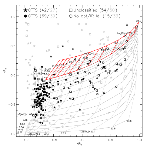
Turning to the remaining 58 sources with less than 50 counts, two show flares (#152 and #376, fig. 14) and are likely to be stars. The others, although maybe a little less spatially concentrated than sources with counterparts, seem to follow a similar distribution in the sky. We conclude that, rather qualitatively, a sizable fraction (of the order of ) of them are associated with NGC 2264. This conclusion is corroborated by the distribution of unidentified sources in the vs. hardness ratio diagram, figure 16. We show for reference a grid of expected loci for absorbed isothermal spectra and the region where power law sources with indexes between 0.9 and 1.9 should lie. Both grids are computed using PIMMS. We note that both (most sensitive to ) and (most sensitive to kT) are on average significantly different for sources with and without counterparts, indicating that non-identified sources are on average characterized by hotter and more absorbed emission. However, the region occupied by about half of the unidentified sources is also occupied by a number of absorbed sources with counterparts, i.e. likely members, while the rest appears to be significantly hotter and possibly compatible with the expected AGN locus.
In conclusion, our 67 sources lacking optical/NIR counterparts are good candidates for new embedded members. Given their absorption these are rather luminous X-ray sources. They are thus unlikely to be low mass stars that have escaped optical/NIR detection because intrinsically fainter than the detection limit. Given the small dependency of on mass (Flaccomio et al., 2003a; Preibisch et al., 2005), low mass stars are indeed usually faint in X-rays. Non-identified sources might be embedded protostars (class I and class 0 objects), medium/high mass very obscured PMS members of NGC 2264 or extragalactic objects shining through the background molecular cloud. They certainly deserve to be followed up with more sensitive IR observations.
6 Results - X-ray activity
Our data indicate that the source of X-ray emission in NGC 2264 low mass members is hot (0.3-10 keV) thermal plasma. The X-ray emission is highly variable in time, the most prominent phenomena being impulsive flares due to magnetic reconnection events. These observations fit well with a solar-like picture of coronal emission and are quite usual for PMS stars. They are, for example, in qualitative agreement with those recently reported for the 1Myr old stars in the ONC by the COUP collaboration (Preibisch et al., 2005). The spectral and temporal characteristics of PMS stars are, broadly speaking, also similar to those of active MS stars, e.g. in the young Pleiades cluster. The most striking differences with respect to MS stars are the X-ray luminosities and the plasma temperatures, both of which are usually found to be higher. As for we note that the fractional X-ray luminosities () are, in PMS stars, comparable or smaller than those of saturated MS stars. Therefore, the higher can be explained by the almost saturated emission of PMS stars and by their larger bolometric luminosities. The higher temperatures might instead indicate a difference in the heating mechanism and/or, a larger contribution to the average flux of flares with hard spectra. At least three questions remain open. First and foremost, the nature of the ultimate mechanism that sustains PMS coronae. While for partially convective MS stars this is identified with the dynamo thanks to the observed relation between activity and stellar rotation, no such evidence is available for PMS stars (Flaccomio et al., 2003a; Preibisch et al., 2005; Rebull et al., 2006). Second, the extent and geometry of coronae, and in particular the possibility of interactions of plasma filled magnetic structures with circumstellar disks (Favata et al., 2005; Jardine et al., 2006). Third, the role of accretion and outflows: soft X-ray emission has been inferred to originate both at the interface between the accretion flow and the photosphere, and within the stellar jets (Kastner et al., 2002; Bally et al., 2003). In this section we now use our data to statistically investigate the dependence of activity, in terms of emission level, variability and spectra, on the stellar and circumstellar characteristics. First however we discuss more in detail the results of our X-ray spectral analysis, with respect to plasma temperatures and absorption values.
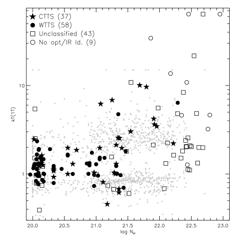
Figure 15 shows the plasma temperature as a function of absorption for all the sources with spectral fits and for which we adopted isothermal models. Figure 17 similarly shows the two best-fit plasma temperatures of sources for which we adopted 2T models. First of all we note that 2T models were required only for , likely because higher column densities absorb the cool component to the extent that it becomes unobservable. Moreover, in the range covered by both models, 2T models were statistically favored in sources with higher statistics while low statistic sources were in most cases successfully fit with a single plasma component with temperature roughly intermediate between those of the two components in 2T models. For 1T models we also note a certain correlation between kT and (fig. 15). While a positive slope of the lower envelope of the datapoints is easily explained as a selection effect, this is not the case for the upper envelope. The paucity of sources with low and high indicates that the X-ray emitting plasma of highly extinct sources is intrinsically hotter than that of optically revealed PMS stars. These hot, highly extinct sources are good candidates for embedded Class 0/I protostars, which have already been suggested to have harder X-ray spectra (Imanishi et al., 2001).
Figure 18 shows, for 2T models, the run of and with stellar mass. Like for the two previously discussed plots, we also show for reference the temperatures obtained by the COUP collaboration (Preibisch et al., 2005) for 1Myr old stars in the ONC252525Note that the COUP observations, obtained with Chandra ACIS, was 850ksec long. The temperatures are thus derived from a spectrum that has been integrated in time over a period that is 8.5 times longer than that of our NGC 2264 observation. With respect to the ONC, in NGC 2264 temperatures appear to be lower on average. This could indicate that at 3Myr, the hot flaring component of the X-ray emission has become less important. It could also result from a lower fraction of CTTSs given that, as we note below (§6.1), CTTS tend to have slightly higher plasma temperatures with respect to WTTS.
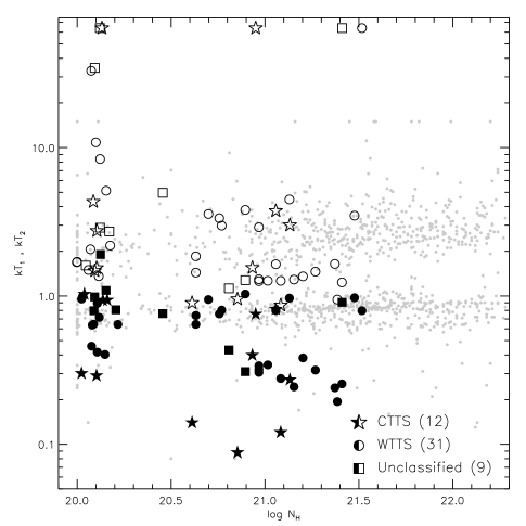
We also note that, with respect to the COUP data, the temperatures that we find for the two isothermal components show a larger scatter. This could be due to: i) larger uncertainties in the NGC 2264 results because of the shorter exposure time and longer distance with respect to the ONC; ii) the shorter exposure time resulting in a larger influence of spectral time variability on the time averaged spectra; iii) a real evolutionary effect (e.g. most ONC stars are CTTS while in NGC 2264 we observe a more varied mixture of CTTS and WTTS); iv) the existence of an additional thermal component that is only sometimes present and/or revealed by the spectral fitting process. In this respect figures 17 and 18 evidence, for sources fit with 2T models, an interesting feature: an apparent separation of the temperatures in two branches, more evident for the cool isothermal component. Taking keV as the dividing line between the two branches, we have 23 and 29 sources in the cool and hot branch respectively. The hot branch has median and of 0.8 and 3.6 keV respectively, roughly coincident with the temperatures of most COUP sources. The cool branch has median and of 0.3 and 1.3keV respectively. Noting that this latter median is similar to the temperatures found for sources that were successfully fit by 1T models, it is reasonable to hypothesize that the EM distributions of these sources have three peaks: one corresponding to the cool keV component that is not present and/or visible for sources in the hot branch, and two peaks at hotter temperatures (i.e. and keV) that are however well represented by an isothermal component with intermediate temperatures. Given the limited statistics of our sources, three component spectral models, although physically reasonable, are not needed and would therefore remain unconstrained by the data.
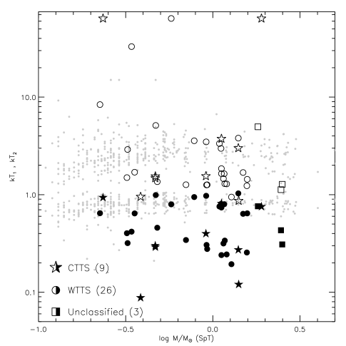
As for the physical origin of the two branches, we note that with respect to the hot branch, stars in the cool branch have lower counts (median counts 270 vs. 630), are significantly less variable according to the KS test (variability fraction 30% vs. 66%, at the 1% confidence level) and are slightly more likely to be CTTS (CTTS fraction: 33% vs. 23%). We note that the difference in variability fractions is unlikely to be explained by statistics alone (c.f. fig 6 and 7). If the 3keV component is due to flaring, it is then possible that the keV component becomes detectable preferentially when flaring is absent and therefore the hot component is suppressed. This soft emission might be physically assimilated to the X-ray emission from the solar corona. This latter would indeed show temperatures similar to 0.3keV if analyzed with ASCA SIS (c.f. Table 1 in Orlando et al., 2001), an instrument with response similar to ACIS. The emission measures we derive for the 0.3keV component of our NGC 2264 sources, ( cm-3) although much larger than those estimated for the Sun, could still be explained by much larger filling factors () and/or larger scale heights of the densest structures (i.e. active region cores).
6.1 Activity in CTTS and WTTS
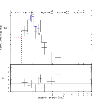
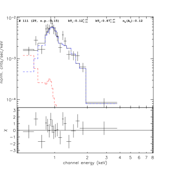
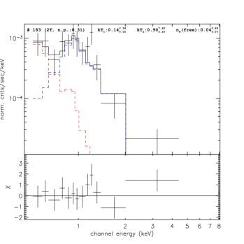
Comparing the plasma temperatures of CTTS and WTTS that are well fit by a single temperature model (37 CTTS, 58 WTTS) we learn that the former are statistically hotter (median: 1.5keV vs. 1.3keV, K-S test probability that the two distributions are compatible: 0.2%). A similar comparison for the two plasma temperatures of stars that required a 2T spectral model (12 CTTS and 31 WTTS) is inconclusive, possibly also because of the lower number of stars. However we have noted above that CTTS appear to be more common among stars with low values of (fig. 17). In particular, the three stars with the lowest are all CTTS. Figure 19 shows the ACIS spectra for these three sources, #17, #111 and #183. The two thermal components of the best fit model are shown separately and the temperatures and absorption are reported from table 6. The most striking case appears to be source #183, which has the highest (0.14keV) and shows a clear double peaked spectrum. The emission measure () of the cool plasma is estimated to be . The other two sources have lower and higher EMs (#17: keV, ; #111: keV, ). We note also that among the three sources #183 has the largest line equivalent width: 27.9 vs. 10.9 and 18.2 for #17 and #111.
As noted in the previous section, low values are usually associated with low . For the three CTTS just discussed for example the values, 0.87-0.95keV, are among the lowest observed and very similar to the cool component for the majority of PMS stars. This suggests that the ultra-cold component is present and/or observable with our spectra only when kev plasma is absent.
A similar trend can be observed for 1T fits (figure 15): among the six lowest kTs (keV), the EW() is know for three stars and in all cases it indicates accretion (i.e. a CTTS). CTTS thus appear to possess both warmer and cooler plasma than WTTS. If this results is confirmed with more statistical significance by further observations, it could imply that the accretion process results in, on one hand, more frequent/energetic flares and, on the other hand, a very cool X-ray plasma produced in the accretion shock (cf. the cases of TW Hydrae and BP Tau: Kastner et al. 2002; Stelzer & Schmitt 2004; Schmitt et al. 2005).
We now investigate the X-ray activity levels ( and ) as a function of bolometric luminosity, stellar mass and accretion properties for the subsample of stars for which stellar masses were derived by placement in the theoretical HR diagram and interpolation of the SDF tracks (160 X-ray detected stars, excluding one possible non-member and two stars outside the tracks). For this investigation we also include upper limits for 16 X-ray undetected likely members (empty symbols in figure 5). Note that a more exhaustive account of the relation between activity and stellar properties, using the X-ray data presented here in conjunction with those of Ramírez et al. (2004a) for another field in NGC 2264, and those of Ramírez et al. (2004b) for the “Orion Flanking Fields”, can be found in Rebull et al. (2006). In that paper the samples for each cluster included many more stars than we have here, but with on average more uncertain stellar parameters. Here we take a different approach, focusing only on the NGC 2264 members in our FOV that are well characterized optically.
Our -mass scatter plot is shown in figure 20. We observe the commonly found mass- correlation (e.g. Rebull et al., 2006), although with a large spread. The position of upper limits indicate that our sensitivity limit is ergs/s, which appears to correspond to a completeness limit in mass at about 0.3-0.4. Moreover we note that, at each stellar mass for which our sample is reasonably complete, CTTS are on average fainter and more scattered with respect to WTTS, confirming the results obtained for ONC stars (Flaccomio et al., 2003a; Preibisch et al., 2005). A similar plot is shown for in Figure 21. appears to be generally high, roughly between and the saturation level . Twenty-two sources actually have measured above the saturation limit. However, a large fraction of these, 73%, are variable, a significantly higher variability fraction than among sources below the saturation threshold (16%). Moreover, most of the sources with the highest values of show large flares, which, if excluded would bring them close or below to the saturation level. Flaccomio et al. (2003a) found evidence for ONC stars of a decrease of at the very lowest masses. Our sample of stars with mass estimates is not complete enough at those masses to study this effect in detail. However, consistently with these results, we do note a decrease in the upper envelope of the vs. mass relation for . Considering CTTS and WTTS separately, the difference in activity is less striking in this plot with respect to the -mass one. However, figure 22 shows, separately for the two PMS classes, the distributions of , both for the whole mass range, and for the subsample with . As noted above, according to the -mass relation, this latter sample should be almost complete. All the distributions take into account upper limits via the Kaplan-Meier estimator. For both samples, and in particular for the mass restricted one, we observe that CTTS are less active with respect to WTTS. Median values differ by 0.32 and 0.41 dex for the two subsamples. The statistical significance of the difference is confirmed by the five two-sample tests in the ASURV package (Feigelson & Nelson, 1985), giving probabilities that the distributions of CTTS and WTTS are taken from the same parent distribution 0.02% for the whole stellar sample and 0.3% for the mass restricted one. We note that this latter result differs from that of Preibisch et al. (2005), who find, in the ONC, a statistically significant difference in the activity levels of CTTS and WTTS only for stars in the 0.2-0.5 mass range.
Finally we repeat with our data the correlation analysis between and performed by Preibisch et al. (2005) for ONC stars classified as CTTS and WTTS. Using the estimation maximization (EM) algorithm in the ASURV package we find very nearly linear correlations between and for the two classes of stars: for WTTS ( dispersion: 0.4 dex) and for CTTS ( dispersion: 0.5 dex). Similarly to the ONC case, accreting stars in NGC 2264 thus appear to be on average fainter than non accreting ones with the same (in this case by a factor of 2) and to have slightly more scattered values. However we note that the power-law slope derived by Preibisch et al. (2005) for accreting stars in the ONC () is significantly shallower than that derived here and that in the ONC the dispersion of points with respect to the best fit relations appear to be larger: 0.5 vs. 0.4 dex for WTTS and 0.7 vs. 0.5 for CTTS. The differences might be be interpreted as an evolutionary effect, given that the ONC is younger than NGC 2264 ( vs. Myr) and that accretion disks are expected to have evolved significantly in the latter cluster (Flaccomio et al., 2003c). We note however that the comparison between the effects of accretion on X-ray activity in the two regions is made uncertain by the different accretion indicators used in the two cases, the and the Ca II equivalent widths for NGC 2264 and the ONC respectively.
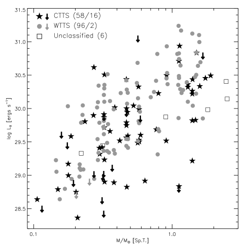
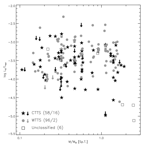

6.2 KH 15D
The peculiar binary system KH 15D has been the subject of many investigations. Herbst & Moran (2005) in particular, analyzing the same X-ray data discussed here conclude that the system is a very weak source of X-ray emission for its mass and age. They tentatively attribute the low X-ray emission to the high eccentricity of the binary system and/or to the close periastron approach of the two stars, that may either disrupt the stellar magnetosphere and/or adversely affect the stellar dynamo.
The X-ray luminosity we derive for KH 15D (our source #309), based on 21.6 detected photons, is 1.3 1029 lower than the value reported by Herbst & Moran (2005) by 0.07 dex. This difference is small and within the uncertainties but, given that the two values are derived from the same X-ray data, we investigated the matter further. The discrepancy can be fully explained by the different estimated number of source photons, 21.6 vs. 22.5, the assumed value of interstellar absorption, vs. cm-2, and the assumed source spectrum.262626Our is based on , derived here from published photometry and spectral type. Herbst & Moran (2005) derive their value from . This should however imply cm-2 assuming and depending on the assumed ratio in the range 1.6-2.0 1021. As for the temperature Herbst & Moran (2005) assume solar abundances and kT=2.7keV, the latter based on the uncertain (due to statistics) hardness ratio. The count to flux conversion factor we used (equation 1) was derived from sources with 50 to 100 counts, which were fit with APEC models with subsolar abundances and median kT of 1.0 keV. Note that our harness ratio analysis (c.f. figure 16) actually indicates a very cool spectrum, kTkeV, with large uncertainties. The 0.07 dex difference in however is not particularly relevant for the physical conclusions regarding the low of the system. KH 15D in not shown in our -mass scatter plot (figure 20) because the system is located in the HR diagram below the grid of the evolutionary tracks (figure 5) and we did not derive a mass. Extrapolating the tracks one would estimate a mass of 0.6-0.7, consistent with the value used by Herbst & Moran (2005), 0.6. Thus placing KH 15D in the -mass diagram we notice that it would fall below the bulk of the other NGC 2264 members, but in an area that is populated by other CTTSs. The value of we derive from our data, -3.45, is moreover perfectly in line with most of the other NGC 2264 members (cf. figure 21). We therefore tend to believe that, rather than being affected by the peculiar binary orbits, the low X-ray emission of KH 15D is due to the same mechanism that suppresses activity in CTTSs.
6.3 Embedded XMM-Newton sources studied by Simon & Dahm (2005)
Simon & Dahm (2005, hereafter SD05) studied in detail three embedded X-ray sources close to IRS 1 (see also §3.3) using XMM-Newton EPIC data taken in March 2002, i.e. 7 months before our ACIS exposure. All the three sources are retrieved in our data and we now compare the results with respect to spectral characteristics, variability and average X-ray luminosities.
EPIC source #26 (our source #194) was the most stable of the three sources. The lightcurves were constant in both observations; the absorption was identical, cm-2; and the kT was also the same within uncertainties272727In this section uncertainties quoted for quantities derived by SD05 are , while for our results we quote 90% confidence intervals.: keV (EPIC) vs. kT= keV (ACIS). The X-ray luminosity however, when corrected for the different energy band used by SD05 (1-10keV vs. our 0.5-7keV) and the different assumed distance (d=800pc, vs. our 760pc) seems to have dropped by a factor between the two observations.
The EPIC source #10 (our source #141) showed a dramatic flare toward the end of SD05’s exposure with the peak count rate reaching 100 times brighter than the quiescent emission before the flare. Our lightcurve is instead compatible with constant emission. DS05 analyzed the spectrum during the flare, while we report results for the average spectrum, which is however built from only photons. There is no evidence of variation in the absorption: DS05 find cm-2 vs. our cm-2. The temperatures are however very different owing to the bright flare in the EPIC data: kT= keV vs. kT= keV. The X-ray luminosities are also very different, with the SD05 value () about 2 dex larger than the value obtained from our analysis and corrected for the different bands and distances. It is therefore likely that we observed the source in a state similar to the pre-flare state in the SD05 data.
Finally, the lightcurve of EPIC source #1 (our source #296) showed, during the XMM exposure, a remarkable rise in count rate by a factor in about 8 ksec, and then began what appears as a slow decay for the remaining 30 ksec of the observation. An isothermal spectral fit gave a very high absorption, cm-2, temperature, kT= keV, and total luminosity ergs s-1 (in the 1-10keV band). From our ACIS data we derive a two order of magnitude smaller luminosity , a somewhat colder plasma, kT= keV and a 5-fold lower absorption cm-2. The lightcurve indicate a roughly linear decay of the count rate during the 100ksec of our observation from cts ksec-1 to cts ksec-1. We note that our value of (90% confidence interval corresponding to ) is roughly in agreement with the absorption SD05 derived for the source from NIR spectroscopy () and, contrary to the value observed during the XMM-Newton exposure, does not imply a gas-to-dust ratio larger than in the interstellar medium. We speculate that the high absorption seen by SD05 is due to a solar-like CME associated with the flare as also speculated for our source #71 in §4.2.
7 Summary and conclusions
We observed NGC 2264 with Chandra-ACIS for 97 ksec, detecting a total of 420 X-ray point sources. We identify 85% of the X-ray sources with known optical and NIR objects, while 67 sources remain with no counterparts in the considered optical/NIR catalogs. More than 90% of the 353 X-ray sources with counterparts are expected to be members of NGC 2264. Using and optical variability data from the literature we select a further sample of 83 X-ray undetected likely members in the FOV of our ACIS observation, bringing the census of likely members with optical/NIR counterparts to 421 stars. Taking into account the small estimated contamination from field stars, we have thus increased the known member census of the region by about 100 objects, mostly very low mass stars and including some candidate brown dwarfs. A further group of 10 X-ray sources, excluded from the member sample because their position in the optical CMD is discrepant with the cluster locus, is also likely to include members. Moreover, among the 67 sources with no optical/NIR counterparts, we argue that about half are previously unrecognized embedded members and good candidates for X-ray detected Class 0/I sources. The other half is instead likely associated with extragalactic objects. The coming SPITZER data, will be very useful to clarify the nature of each source and will allow a systematic study of X-ray activity in the protostellar phase.
We determined X-ray unabsorbed fluxes and luminosities for 326 sources for which absorption could be estimated, either from the X-ray spectra, from optical spectral types and photometry () or from NIR photometry. With the aim of shedding light on PMS X-ray activity, we then performed a detailed study of X-ray lightcurves and spectra, and studied the relation between the properties of X-ray emitting plasma and stellar/circumstellar characteristics. We confirm several previous findings: X-ray luminosity is related to bolometric luminosity and to stellar mass; is on average high and rather independent of mass, other than for a possible drop at and a shallow decrease for . The mass- relation appears to be better defined for WTTS than for CTTS, and CTTS have on average lower activity levels at any given bolometric luminosity and mass. We found tentative evidence that CTTS are more time variable with respect to WTTS, which might be related to the time-variable nature of the accretion process if this latter plays a role in the X-ray emission. With respect to spectral characteristics, the plasma on CTTS is on average slightly hotter than on WTTS, a finding possibly related to the higher variability of CTTS. However, we also observe that the sources with the coolest plasma are preferentially CTTS. Three CTTSs in particular appear to have plasma at keV, i.e. comparable with the temperatures expected for plasma heated by accretion shocks, as observed on TW Hydrae (keV, Kastner et al., 2002; Stelzer & Schmitt, 2004). The estimated emission measures of this cool plasma is between 4 and 17 times larger than on TW Hydrae ( cm-3), maybe as a result of the expected larger accretion rates of NGC 2264 stars. These results, taken as a whole, reinforce the mounting evidence that activity in low mass PMS stars, while generally similar to that of saturated MS stars, is significantly affected by mass accretion. This influence has at least two aspects: accretion is on one hand a positive source of very soft X-ray emission produced in the accretion shock. On the other hand it reduces the average energy output of coronae and makes the emission more time variable. Preibisch et al. (2005) discuss several possible explanations for the suppression of activity. They favor the idea that accretion modifies the magnetic field geometry and results in the “mass-loading” of field lines, thus hampering the heating of plasma to X-ray temperatures. It is at the same time conceivable that the resulting magnetic field structure will be more unstable because of the the temporal variability of the mass accretion rate as well as the rotational shear at the inner edge of the circumstellar disk. In order tackle the so-far elusive activity-accretion relation, a better characterization of the circumstellar/accretion properties, e.g. measures of mass accretion rates, is essential. Particularly useful in these respect would be contemporary observations in the X-ray band and in accretion/outflow sensitive optical/NIR lines.
Acknowledgements.
The authors wish to tank the anonymous referee that with his comments helped to improve this work and acknowledge financial support from the Ministero dell’Istruzione dell’Universitá e della Ricerca, PRIN-INAF and contract ASI-INAF I/023/05/0.References
- Alexander et al. (2003) Alexander, D. M., et al. 2003, AJ, 126, 539
- Bally et al. (2003) Bally, J., Feigelson, E., & Reipurth, B. 2003, ApJ, 584, 843
- Barger et al. (2003) Barger, A. J., et al. 2003, AJ, 126, 632
- Dahm & Simon (2005) Dahm, S. E., & Simon, T. 2005, AJ, 129, 829
- Damiani et al. (1997) Damiani, F.,Maggio, A., Micela, G., & Sciortino, S. 1997, ApJ, 483, 350
- Damiani & Micela (1995) Damiani, F., & Micela, G. 1995, ApJ, 446, 341
- Favata & Schmitt (1999) Favata, F., & Schmitt, J. H. M. M. 1999, A&A, 350, 900
- Favata et al. (2005) Favata, F., Flaccomio, E., Reale, et al., ApJS, 160, 469
- Feigelson & Nelson (1985) Feigelson, E. D., & Nelson, P. I. 1985, ApJ, 293, 192
- Flaccomio et al. (2000) Flaccomio, E., Micela, G., Sciortino, S., et al. 2000, A&A, 355, 651
- Flaccomio et al. (2003a) Flaccomio, E., Damiani, F., Micela, G., et al. 2003, ApJ, 582, 398
- Flaccomio et al. (2003b) Flaccomio, E., Micela, G., & Sciortino, S. 2003, A&A, 397, 611
- Flaccomio et al. (2003c) Flaccomio, E., Micela, G., & Sciortino, S. 2003, A&A, 402, 277
- Flaccomio et al. (2005) Flaccomio, E., Micela, G., Sciortino, S., et al., 2005, ApJS, 160, 450
- Getman et al. (2005) Getman, K. V., et al. 2005, ApJS, 160, 319
- Glassgold et al. (2004) Glassgold, A. E., Najita, J., & Igea, J. 2004, ApJ, 615, 972
- Haisch et al. (2005) Haisch, K. E., Jayawardhana, R., & Alves, J. 2005, ApJ, 627, L57
- Hamilton et al. (2005) Hamilton, C. M., et al. 2005, AJ, 130, 1896
- Herbst & Moran (2005) Herbst, W., & Moran, E. C. 2005, ApJ, 630, 400
- Igea & Glassgold (1999) Igea, J., & Glassgold, A. E. 1999, ApJ, 518, 848
- Imanishi et al. (2001) Imanishi, K., Koyama, K., & Tsuboi, Y. 2001, ApJ, 557, 747
- Jardine et al. (2006) Jardine, M., Collier Cameron, A., Donati, J. -., Gregory, S. G., & Wood, K. 2006, ArXiv Astrophysics e-prints, arXiv:astro-ph/0601213
- Kastner et al. (2002) Kastner, J. H., Huenemoerder, D. P., Schulz, N. S., Canizares, C. R., & Weintraub, D. A. 2002, ApJ, 567, 434
- Kenyon & Hartmann (1995) Kenyon, S. J. & Hartmann, L. 1995, ApJS, 101, 117
- Kenyon & Hartmann (1995) Kenyon, S. J., & Hartmann, L. 1995, ApJS, 101, 117
- Lada (2006) Lada, C. J. 2006, ArXiv Astrophysics e-prints, arXiv:astro-ph/0601375
- Lamm et al. (2004) Lamm, M. H., Bailer-Jones, C. A. L., Mundt, R., Herbst, W., & Scholz, A. 2004, A&A, 417, 557
- Lorenzani & Palla (2001) Lorenzani, A., & Palla, F. 2001, ASP Conf. Ser. 243: From Darkness to Light: Origin and Evolution of Young Stellar Clusters, 243, 745
- Luhman (1999) Luhman, K. L. 1999, ApJ, 525, 466
- Margulis et al. (1989) Margulis, M., Lada, C. J., & Young, E. T. 1989, ApJ, 345, 906
- Meyer et al. (1997) Meyer, M. R., Calvet, N., & Hillenbrand, L. A. 1997, AJ, 114, 288
- Orlando et al. (2001) Orlando, S., Peres, G., & Reale, F. 2001, ApJ, 560, 499
- Palla & Stahler (2000) Palla, F., & Stahler, S. W. 2000, ApJ, 540, 255
- Park et al. (2000) Park, B., Sung, H., Bessell, M. S., & Kang, Y. H. 2000, AJ, 120, 894
- Peretto et al. (2006) Peretto, N., André, P., & Belloche, A. 2006, A&A, 445, 979
- Pizzolato et al. (2003) Pizzolato, N., Maggio, A., Micela, G., Sciortino, S., & Ventura, P. 2003, A&A, 397, 147
- Preibisch et al. (2005) Preibisch, T., et al. 2005, ApJS, 160, 401
- Ramírez et al. (2004a) Ramírez, S. V., et al. 2004, AJ, 127, 2659
- Ramírez et al. (2004b) Ramírez, S. V., et al. 2004, AJ, 128, 787
- Rebull et al. (2002) Rebull, L. M., Makidon, R. B., Strom, S. E., et al. 2002, AJ, 123, 1528
- Rebull et al. (2006) Rebull, L. M., Stauffer, J. R., Ramirez, S. V., et al. 2006, ArXiv Astrophysics e-prints, arXiv:astro-ph/0603027
- Rieke & Lebofsky (1985) Rieke, G. H., & Lebofsky, M. J. 1985, ApJ, 288, 618
- Salpeter (1955) Salpeter, E. E. 1955, ApJ, 121, 16
- Schreyer et al. (2003) Schreyer, K., Stecklum, B., Linz, H., & Henning, T. 2003, ApJ, 599, 335
- Schmitt & Liefke (2004) Schmitt, J. H. M. M., & Liefke, C. 2004, A&A, 417, 651
- Schmitt et al. (2005) Schmitt, J. H. M. M., Robrade, J., Ness, J.-U., Favata, F., & Stelzer, B. 2005, A&A, 432, L35
- Siess et al. (2000) Siess, L., Dufour, E., & Forestini, M. 2000, A&A, 358, 593
- Simon & Dahm (2005) Simon, T., & Dahm, S. E. 2005, ApJ, 618, 795
- Stelzer & Schmitt (2004) Stelzer, B., & Schmitt, J. H. M. M. 2004, A&A, 418, 687
- Sung et al. (1997) Sung, H., Bessell, M. S., & Lee, S.-W. 1997, AJ, 114, 2644
- Teixeira et al. (2006) Teixeira, P. S., et al. 2006, ArXiv Astrophysics e-prints, arXiv:astro-ph/0511732
- Vasilevskis et al. (1965) Vasilevskis S., Sanders W.L., Balz A.G.A.J., 1965, AJ 70, 797
- Vuong et al. (2003) Vuong, M. H., Montmerle, T., Grosso, et al. 2003, A&A, 408, 581
- Walker (1956) Walker M. F., 1956, ApJS 2, 365
- Williams & Garland (2002) Williams, J. P. & Garland, C. A. 2002, ApJ, 568, 259
- Wilms et al. (2000) Wilms, J., Allen, A., & McCray, R. 2000, ApJ, 542, 914
- Young et al. (2006) Young, E. T., et al. 2006, ArXiv Astrophysics e-prints, arXiv:astro-ph/0601300