Bayesian foreground analysis with CMB data

Abstract

The quality of CMB observations has improved dramatically in the last few years, and will continue to do so in the coming decade. Over a wide range of angular scales, the uncertainty due to instrumental noise is now small compared to the cosmic variance. One may claim with some justification that we have entered the era of precision CMB cosmology. However, some caution is still warranted: The errors due to residual foreground contamination in the CMB power spectrum and cosmological parameters remain largely unquantified, and the effect of these errors on important cosmological parameters such as the optical depth $\tau$ and spectral index $n_{\textrm{s}}$ is not obvious. A major goal for current CMB analysis efforts must therefore be to develop methods that allows us to propagate such uncertainties from the raw data through to the final products. Here we review a recently proposed method that may be a first step towards that goal.

1 Introduction

The great importance of the foreground problem for CMB studies has long been recognized in the cosmological community, and as a result a large number of algorithms have been proposed, implemented and applied to both simulated and real data. Examples are the Maximum Entropy Method (Barreiro et al., 2004; Bennett et al., 2003b; Hobson et al., 1998; Stolyarov et al., 2002, 2005), Internal Linear Combination methods (Bennett et al., 2003b; Tegmark et al., 2003; Eriksen et al., 2004a; Saha et al., 2005; Hansen et al., 2006; Hinshaw et al., 2006), Wiener filtering (Bouchet & Gispert, 1999; Tegmark & Efstathiou, 1996), Independent Component Analysis methods (Maino et al., 2002, 2003; Donzelli et al., 2005) and spectral fitting approaches (Delabrouille et al., 2003).

The main emphasis of most of these methods lies on establishing an optimal estimate of the CMB sky signal, and not so much on quantifying the uncertainty on that estimate. A different approach was taken by Brandt et al. (1994) who simply adopted well-established likelihood parameter estimation techniques to solve the problem. Ten years later this work was continued by Eriksen et al. (2006), by taking advantage of recent statistical (in particular Markov Chain Monte Carlo) and computational developments.

In this paper we briefly review the algorithm as presented by Eriksen et al. (2006). We then describe three applications, namely 1) an analysis of simulated Planck + six-year WMAP data, 2) a preliminary analysis of the first-year WMAP data, and 3) a preliminary study of experimental design.

2 Methods

The most straightforward method for producing reliable error bars is provided by standard parameter estimation techniques. In particular, the Bayesian framework is particularly suited for this type of problem.

Given a set of observed data $\mathbf{d}$ and an assumed model $\mathbf{s}(\theta)$, $\theta$ being a general set of parameters, we simply ask, what is the posterior distribution $P(\theta|\mathbf{d})$? To answer this, we first recall Bayes’ formula,

$$P(\theta|\mathbf{d})\propto P(\mathbf{d}|\theta)P(\theta)=\mathcal{L}(\theta)P(\theta),$$ (1)

where $\mathcal{L}(\theta)\equiv P(\mathbf{d}|\theta)$ is the likelihood and $P(\theta)$ is a prior summarizing our previous knowledge about $\theta$. For Gaussian data, the likelihood is given by

$$-2\ln\mathcal{L}=\chi^{2}(\theta)=\left[\mathbf{d}-\mathbf{s}(\theta)\right]^{t}\mathbf{C}^{-1}\left[\mathbf{d}-\mathbf{s}(\theta)\right],$$ (2)

where $\mathbf{C}$ is the covariance matrix, up to an irrelevant constant. (In the current implementation, we assume no pixel-pixel correlations, and $\mathbf{C}=\mathbf{N}$ is defined to be the noise covariance matrix.) The problem is thus reduced to mapping out the posterior as a function of the free parameters $\theta$ using some computational tool, such as MCMC or grid evaluations.

Figure 1: Marginalized posterior distributions for six parameters fitted to a single pixel by Markov Chain Monte Carlo. This example is taken from a simulation corresponding to the combination of Planck and six-year WMAP, for a pixel located exactly on the Galactic plane. The vertical lines indicate the true parameter values. (Note that this is not a well-defined quantity for the dust spectral index, since we fit for a one-component dust model whereas the simulation is based on a two-component dust model.)

This machinery may be applied to microwave component reconstruction by noting that different signal components have different spectral and spatial behaviour. By observing the sky in different frequencies and directions one may disentangle the various contributions and isolate the CMB signal.

The first step is therefore to choose a suitable parametric model. For CMB analysis, a particularly convenient choice is that of a sum of independent modulated power-law components,

$$S(\nu;\theta) =\sum_{i=1}^{N_{\textrm{comp}}}S_{i}(\nu;\theta_{i})$$ (3)

$$=\sum_{i=1}^{N_{\textrm{comp}}}A_{i}f_{i}(\nu)\left(\frac{\nu}{\nu_{0,i}}\right)^{\beta_{i}}.$$ (4)

Here one typically would include a CMB term ($A_{\textrm{cmb}}=T_{\textrm{cmb}}$; $f_{\textrm{cmb}}(\nu)$ is the thermodynamic-to-antenna temperature conversion factor; $\beta_{\textrm{cmb}}\equiv 0$), a synchrotron and free-free term ($A$ and/or $\beta$ free parameters; $f_{\textrm{s}}(\nu)=1$), and a thermal dust term.

These few simple definitions summarize the method quite succinctly. No a priori assumptions about the sky emission are required, except that it can be represented by a parametric model. The remaining discussion is concerned mostly about how to deal with real-world complications such as limited spectral information, low signal-to-noise ratio, and computational constraints. It is worth emphasizing that even an unrealistically simple sky model containing nothing but CMB, free-free, synchrotron, and dust emission requires at least six parameters, and that no CMB experiment to date has had even the eight frequencies required to fit such a minimal model. Fortunately, the method can be extended easily to include other information, as will be seen in the next section.

2.1 Calibration and template fitting

Two major complications arise when trying to apply the above machinery to real-world data. First, spectral fits generally require that all sky maps are properly calibrated with respect to a common zero-point. This is not trivial for any CMB experiment, and certainly not for differential observatories such as the WMAP satellite. Second, as previously mentioned, the number of observed frequencies is often (i.e., in every experiment performed to date!) smaller than the number of parameters one might wish to include. For instance, WMAP observes the sky at five frequencies, while, ideally, we would like to include at least six parameters in a reasonable model (CMB, synchrotron, free-free and thermal dust amplitudes, and synchrotron and dust spectral indicies), still neglecting a possible anomalous dust contribution.

A straightforward way to address both problems is to introduce template terms in the signal model,

$$\begin{split}S(\nu;\theta)\rightarrow S(\hat{n},\nu;\theta)=\quad\quad\quad\quad\quad\quad\quad\\ =\sum_{i=1}^{N_{\textrm{pix}}}S(\nu;\theta_{i})+\sum_{i=1}^{N_{\textrm{temp}}}A_{i}(\nu)g_{i}(\hat{n}).\end{split}$$ (5)

That is, in addition to the previously defined (and usually rather complicated) spectral models, we also fit for a small set of global (and simple) template amplitudes. Common templates to include would be a monopole term, three dipole terms, and either reasonably well-behaved (e.g,. free-free emission through an H_α template) or sub-dominant (e.g., thermal dust emission for WMAP) foreground components. For each signal component one is able to handle this way, one saves one degree of freedom in all subsequent non-linear fits, thus obtaining very useful additional stability.

The cost of this approach is that the problem becomes global, and the computational load is vastly increased. At present it is therefore only feasible to perform such an analysis at low resolution and with a non-linear search. Nevertheless, since the main target at this stage is a relatively small number of global template amplitudes, little is lost by this approach.

Note that this extension of the method was discussed only briefly by Eriksen et al. (2006) in the context of monopole and dipole calibration, not general template fits, and it was also not implemented at that time. The analysis of the first-year WMAP data presented in this paper is therefore the first application of the method.

2.2 Estimating spectral indices from low-resolution maps

After calibrating and removing well-behaved components from the maps using the above description, the next step is to map out the full posterior for each pixel with low-resolution maps. The reasons for using low-resolution maps at this stage are two-fold: On the one hand, estimation of non-linear parameters such as spectral indices is quite sensitive to noise, and it is therefore highly desirable to have high signal-to-noise data. On the other hand, we use full-blown MCMC to map out the posteriors for each pixel, and with a computational cost of about 100 CPU-seconds per pixel it is currently not feasible to do this for mega-million pixel maps.

Figure 2: Simulation constructed to test the algorithm based on a semi-realistic model of the foregrounds: The synchrotron emission includes spatial variations in the spectral index (Giardino et al., 2002), and the thermal dust emission follows the two-component “model 8” of Finkbeiner et al. (1999). For further information on this simulation, see Eriksen et al. (2006).

For these two reasons, we smooth each map with a wide beam (typically with a Gaussian beam of, say, $7^{\circ}$ FWHM) and downgrade the pixel resolution (typically to, say, $2^{\circ}$ pixel size; $N_{\textrm{side}}=32$ in HEALPix language) prior to the MCMC analysis. The computational expense is then quite manageable with a modern-type cluster, with a total cost of about 500 CPU hours.

The final product from this stage is a single joint probability distribution for each pixel, and from these we find the univariate distributions for each parameter by marginalizing over all others. Examples of such univariate distributions are shown in Figure 1. Finally, we store the posterior mean and variance for each parameter and each pixel in the form of two sky maps as our final data products.

2.3 Estimating amplitudes from high-resolution maps

Figure 3: Full-sky results obtained from the simulation described in Section 3.1. Shown are reconstructed parameter values (left column), actual residual errors (middle column), and estimated uncertainties (right column). The sharp boundaries are caused by different assumed models (e.g., free-free is omitted from the fitting model at high latitudes but included at low), which leads to order-of-magnitude different uncertainties because of degeneracies.

While the procedure described in the previous section gives a full representation of the posteriors for the low-resolution sky maps, we also want a good representation of the full-resolution posteriors. To obtain these, we make the assumption that the spectral indices vary more slowly than the amplitudes, and fix their distributions at the corresponding low-resolution values. Given the values of all non-linear parameters, the likelihood becomes Gaussian, and the analysis may be performed analytically with modest computational expenses. For details on this procedure, see Eriksen et al. (2006).

3 Example applications

In the following sections, we show a few demonstrations of how this method performs in practice. First, we review the simulation described by Eriksen et al. (2006). We then show the results from a preliminary analysis of the first-year WMAP data. We emphasize that these results are preliminary, and will be revised with the currently available three-year data. Finally, we show some early results from a currently on-going study of optimization of future experiments.

3.1 Planck + six-year WMAP simulation

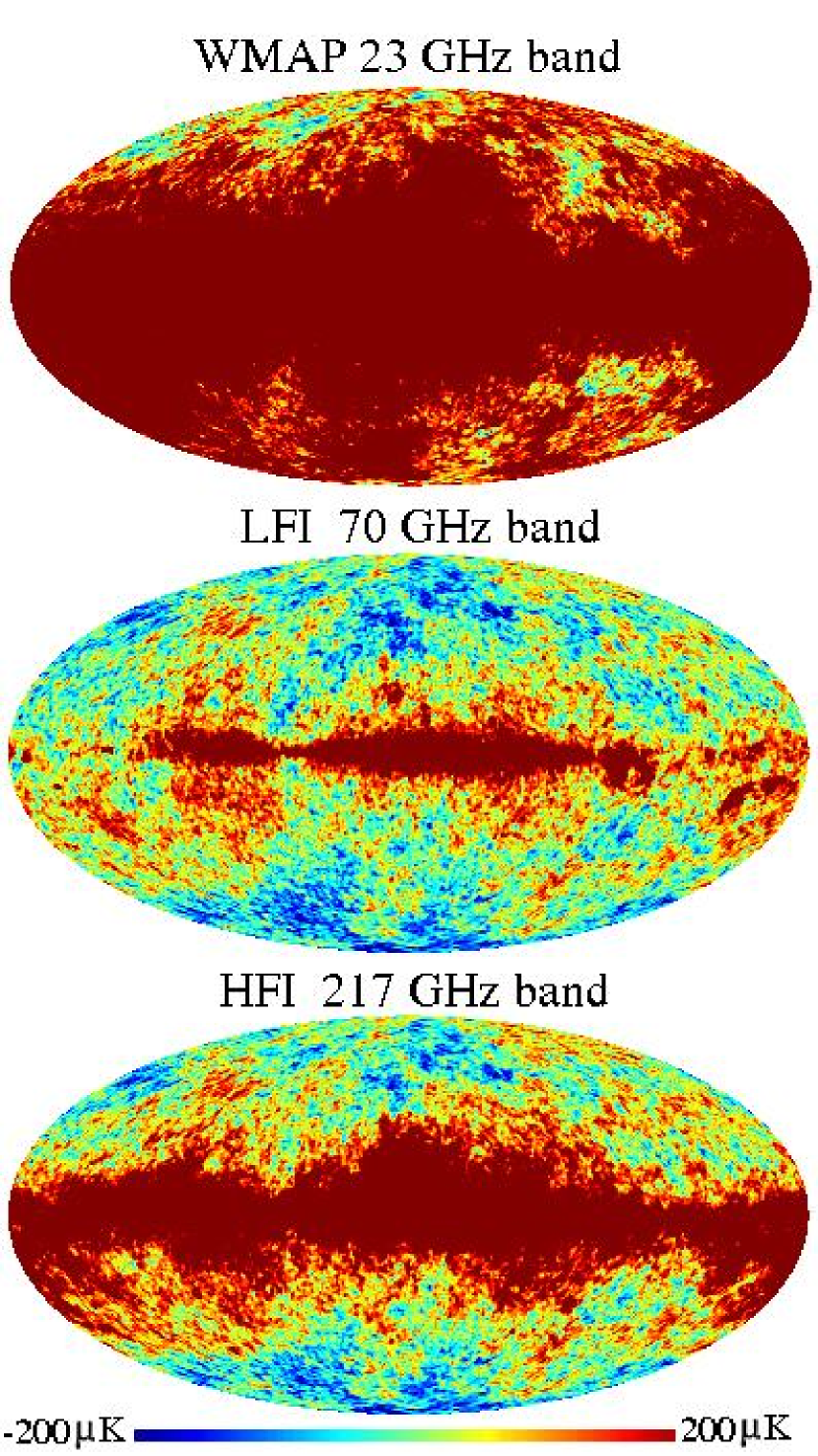
In order to test the algorithm, Eriksen et al. (2006) constructed a simulation corresponding to a combination of six Planck channels (30 to 217 GHz) and five WMAP channels (23 to 94 GHz). The higher-frequency Planck channels were not included because of modelling error confusion associated with including multiple dust components. The simulation took into account the beam and white noise characteristics of each channel separately. Four signal components were included: a Gaussian CMB realization drawn from the best-fit WMAP $\Lambda$CDM power spectrum; a semi-realistic synchrotron component, featuring a spatially varying spectral index (Giardino et al., 2002); a free-free component with fixed spectral index of $\beta_{\textrm{ff}}=-2.15$ (Dickinson et al., 2003); and a two-component thermal dust model (“model 8” of Finkbeiner et al. 1999). Thus, the simulation includes two major complications that we must expect to find in real data, namely both spatially varying spectral indices and departures from simple power law spectra. Three selected channel maps are shown in Figure 2.

These simulations were then analyzed using the machinery described above. The results are discussed in detail in the original paper; two sample results are reprinted here. In Figure 1 we show the marginal densities for one single pixel located exactly on the Galactic plane, and the true values for each parameter is marked by a solid line. Clearly, the posterior distributions agree very well with the input values, both in mean and variance.

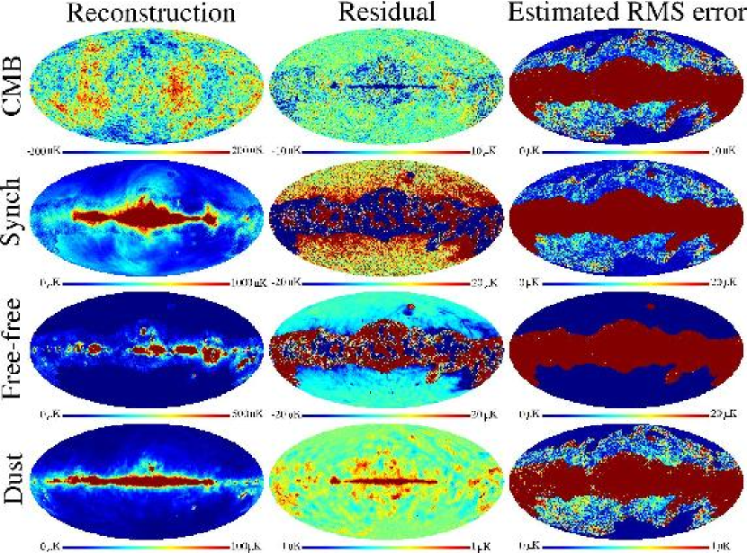
In Figure 3 we show sky maps of the four component amplitudes that were estimated: Posterior means are shown in the left column, actual residuals are shown in the middle column, and estimated errors are shown in the right column. Again, the results agree very well with expectations.

3.2 The first-year WMAP data

In this section we present for the first time the results from a parametric foreground analysis of the first-year WMAP data (Bennett et al., 2003a). These data comprise a set of full-sky temperature maps at five frequencies (23, 33, 41, 61 and 94 GHz) at angular resolutions between $13^{\prime}$ and $53^{\prime}$ FWHM. The noise is assumed to be white, and all beams are assumed to be circularly symmetric.

As described above, the analysis was performed in three stages, two at low resolution ($7^{\circ}$ FWHM for WMAP), and the third at high resolution ($1^{\circ}$). In the first or calibration stage, the free parameters were a monopole and dipole amplitude, a free-free template amplitude (Finkbeiner, 2003), and a dust template amplitude (Finkbeiner et al., 1999) for each band, and a CMB temperature and a synchrotron amplitude and spectral index for each pixel. The fit was performed using a non-linear Sequential Quadratic Programming (SQP) algorithm.

In the second stage, the low-resolution posterior distributions are mapped out using MCMC. Only CMB and synchrotron (both amplitude and spectral index) were included in this case. The main result from these computations is a synchrotron spectral index map, shown in the bottom panel of Figure 4. Note that the most values lie between $-2.0$ and $-3.4$, which is quite acceptable. (Values larger than $-2.3$ probably indicate residual free-free emission, rather than break-down in the synchrotron estimation.)

Figure 4: Results from first-year WMAP analysis. Shown are reconstructed CMB signal (top panel), synchrotron amplitude (middle panel), and synchrotron spectral index (bottom panel).

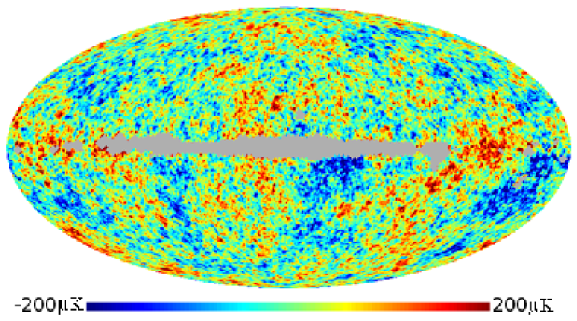
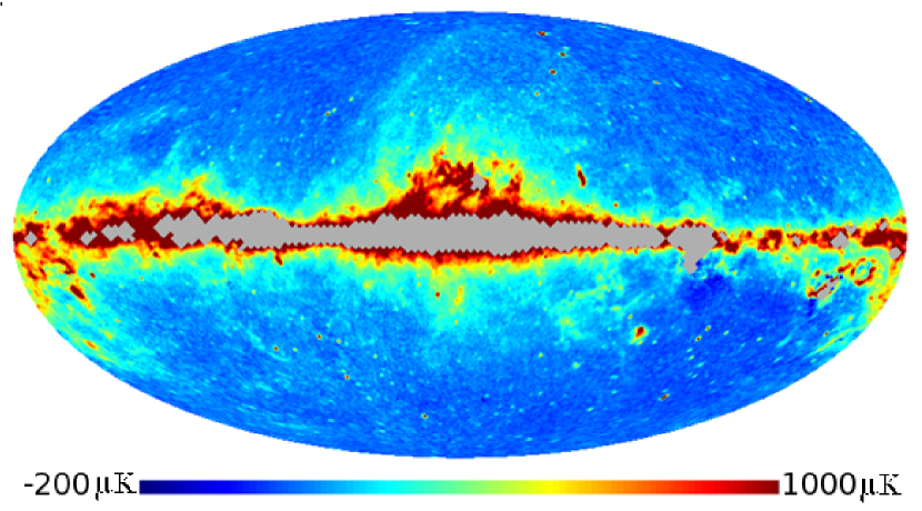
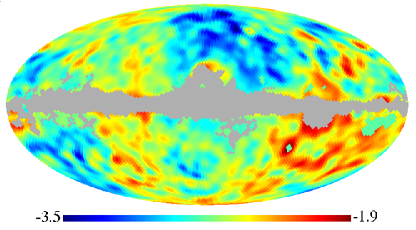
In the third stage, we estimate the CMB and synchrotron amplitudes analytically. The results from these calculations are shown in the two panels of Figure 4. (The synchrotron amplitude is normalized to K band.) Again, the results appear visually quite compelling, although a more quantitative analysis is warranted. However, we re-emphasize that these results are presented only to demonstrate the capabilities of the method, and not as definitive measurements. The analysis will soon be revisited based on the recently available three-year WMAP data.

3.3 Experiment design

The machinery described in Section 2 is also very well suited to study optimization of future experiments. The question we want to answer is, given a set of instrumental constraints (e.g., focal plane area and power dissipation) how should we distribute the number of detectors as a function of frequency in order to optimize our ability to extract the CMB signal?

One possible method for answering this question would be to apply the above machinery to a wide range of allowed instrument configurations, and study how the uncertainties (or residuals) change with configuration. In a currently on-going project, we try to do this in a systematic fashion, and in this section we present some very preliminary results from this study.

Figure 5: Example results from the experimental design study. The curves represent different configurations allowed by the experimental constraints, and show the effective noise per frequency channel, which is directly related to the number of detectors per frequency. The thickness (and color) indicates the reconstruction quality: A thicker (and redder) line indicates a better reconstruction. The optimal solution here is the thick red line, which corresponds to a constant signal-to-noise ratio.

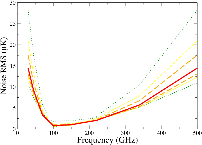
We consider a generalized version of the simulations described in Section 3.1, for which the frequency bands and the noise RMS per frequency may be chosen freely. We then impose a set of constraints corresponding to the focal plane area of an optical system that could fly in space, and feeds at different frequencies of realistic size. Based on these constraints, we generate a grid of possible instrument configurations, and run the analysis for a reasonable set of these. (Most may be discarded by common sense.)

A few example results are shown in Figure 5: The lines indicate the noise RMS distribution as a function of frequency ($\sigma(\nu)=\sigma_{0}(\nu)/\sqrt{N_{\textrm{det}}(\nu)}$, where $N_{\textrm{det}}$ is the number of detectors at frequency $\nu$) for seven different configurations. The thickness (and color) of the lines indicates the resulting uncertainty/residual from the component separation: A thicker (redder) line means a better reconstruction. The optimal distribution of detectors among this set is therefore the solid red line.

From this simple exercise, we may formulate a first design principle: The optimal noise distribution is the one that corresponds to a constant signal-to-noise ratio, where the signal is the sum of CMB and foregrounds. Second, the wider the frequency coverage, the better the reconstruction.

However, there is a major caveat here: This principle only holds when any modelling errors (i.e., errors due to the fact that the assumed parametric model is different from the true signal) are small. Performing a similar exercise on simulations with significant modelling errors results in a competing principle: When the parametric shape of the foreground components are poorly known, the best reconstructions are obtained with configurations surrounding the foreground minimum. The optimal total frequency span depends on the magnitude of the modelling errors. Both of these principles sound rather obvious, but they are nevertheless worth making explicit.

In conclusion, two competing effects are at work: Reconstruction power is maximized by a wide frequency coverage, but limited by modelling errors. In a future publication, we will quantify these considerations in much greater detail, and attempt to provide some guidelines on the preferred frequency ranges for future CMB experiments. Firm conclusions, however, will require an understanding of modelling errors based on better knowledge of the foregrounds themselves, knowledge that can come only from measurements of the polarized sky over a broad range of frequencies with great sensitivity.

4 Discussion

As the sensitivity of CMB observations continue to improve, the importance of properly characterizing the foreground contributions also increases. Even with WMAP we are already at a level where instrumental noise is negligible compared to the foreground uncertainties over a wide range of angular scales (Hinshaw et al., 2006), and this will be even more true for Planck and up-coming polarization experiments. Simple template corrections will be hopelessly inadequate to reach the required sensitivity levels. Further, it will be essential to propagate the foreground uncertainties through to the final products, namely the CMB power spectrum and cosmological parameters.

On this background, we argue that the most appropriate solution will be based on traditional parameter estimation techniques, rather than image processing techniques. The reason is simply that such methods naturally provide the full posterior distributions, and are integrated easily with existing power spectrum and parameter estimation methods based on Bayesian parameter estimation. An approach that appears particularly promising in this respect is that of Gibbs sampling, which allows for joint global analysis of foregrounds, CMB power spectrum and even cosmological parameters (Jewell et al., 2004; Wandelt et al., 2004; Eriksen et al., 2004b, 2006).

In fact, we end by emphasizing that the particular implementation we describe in this paper is of less importance than its underlying idea. Many improvements can be made to the algorithm as such (e.g., introducing support for spatial correlation information would be of great value), but our main conclusion is independent of such details: CMB component separation is a probabilistic problem, and obtaining accurate uncertainties is a crucial part of the problem. Parameter estimation techniques provide the most direct route for doing so.

References

- Barreiro et al. (2004) Barreiro, R. B., Hobson, M. P., Banday, A. J., Lasenby, A. N., Stolyarov, V., Vielva, P., & Górski, K. M. 2004, MNRAS, 351, 515
- Bennett et al. (2003a) Bennett, C. L. et al. 2003a, ApJS, 148, 1
- Bennett et al. (2003b) Bennett, C. L. et al. 2003b, ApJS, 148, 97
- Bouchet & Gispert (1999) Bouchet, F. R., & Gispert, R. 1999, New Astronomy, 4, 443
- Brandt et al. (1994) Brandt, W. N., Lawrence, C. R., Readhead, A. C. S., Pakianathan, J. N., & Fiola, T. M. 1994, ApJ, 424, 1
- Delabrouille et al. (2003) Delabrouille, J., Cardoso, J.-F., & Patanchon, G. 2003, MNRAS, 346, 1089
- Dickinson et al. (2003) Dickinson, C., Davies, R. D., & Davis, R. J. 2003, MNRAS, 341 369
- Donzelli et al. (2005) Donzelli, S., et al., 2005, MNRAS, submitted, [astro-ph/0507267]
- Eriksen et al. (2004a) Eriksen, H. K., Banday, A. J., Górski, K. M., Lilje, P. B. 2004a, ApJ, 612, 633
- Eriksen et al. (2004b) Eriksen, H. K., et al. 2004b, ApJS, 155, 227
- Eriksen et al. (2006) Eriksen, H. K., et al. 2006, ApJ, 641, 665, [astro-ph/0508268]
- Finkbeiner et al. (1999) Finkbeiner, D. P., Davis, M., & Schlegel, D. J. 1999, ApJ, 524, 867
- Finkbeiner (2003) Finkbeiner, D. P. 2003, ApJS, 146, 407
- Giardino et al. (2002) Giardino, G., Banday, A. J., Górski, K. M., Bennett, K., Jonas, J. L., & Tauber, J. 2002, A&A, 387, 82
- Górski et al. (2005) Górski, K. M., Hivon, E., Banday, A. J., Wandelt, B. D., Hansen, F. K., Reinecke, M., &Bartelmann, M. 2005, ApJ, 622, 759
- Hansen et al. (2006) Hansen, F. K., Banday, A. J., Eriksen, H. K., Gorski, K. M., & Lilje, P. B. 2006, ApJ, submitted, [astro-ph/0603308]
- Hinshaw et al. (2006) Hinshaw, G., et al. 2006, ApJ, submitted, [astro-ph/0603451]
- Hobson et al. (1998) Hobson, M. P., Jones, A. W., Lasenby, A. N., & Bouchet, F. R. 1998,MNRAS, 300, 1
- Jewell et al. (2004) Jewell, J., Levin, S., & Anderson, C. H. 2004, ApJ, 609, 1
- Maino et al. (2002) Maino, D., et al. 2002, MNRAS, 334, 53
- Maino et al. (2003) Maino, D., Banday, A. J., Baccigalupi, C., Perrotta, F., & Górski, K. M. 2003, MNRAS, 344, 544
- Saha et al. (2005) Saha, R., Jain, P., & Souradeep, T. 2005, [astro-ph/0508383]
- Stolyarov et al. (2002) Stolyarov, V., Hobson, M. P., Ashdown, M. A. J., & Lasenby, A. N. 2002, MNRAS, 336, 97
- Stolyarov et al. (2005) Stolyarov, V., Hobson, M. P., Lasenby, A. N., & Barreiro, R. B. 2005, MNRAS, 357, 145
- Tegmark & Efstathiou (1996) Tegmark, M., & Efstathiou, G. 1996, MNRAS, 281, 1297
- Tegmark et al. (2003) Tegmark, M., de Oliveira-Costa, A., & Hamilton, A. J. 2003, Phys. Rev. D, 68, 123523
- Wandelt et al. (2004) Wandelt, B. D., Larson, D. L., & Lakshminarayanan, A. 2004, Phys. Rev. D, 70, 083511