UV Radiative Feedback on High–Redshift Proto–Galaxies

Abstract

We use three-dimensional hydrodynamic simulations to investigate the effects of a transient photoionizing ultraviolet (UV) flux on the collapse and cooling of pregalactic clouds. These clouds have masses in the range $10^{5}$ – $10^{7}~{}M_{\odot}$, form at high redshifts ($z\mathrel{\hbox to0.0pt{\lower 4.0pt\hbox{\hskip 1.0pt$\sim$}\hss}\raise 1.0pt\hbox{$>$}}18$), and are assumed to lie within the short–lived cosmological HII regions around the first generation of stars. In addition, we study the combined effects of this transient UV flux and a persistent Lyman–Werner (LW) background (at photon energies below 13.6eV) from distant sources. In the absence of a LW background, we find that a critical specific intensity of $J_{\rm UV}\sim 0.1\times 10^{-21}{\rm ergs~{}s^{-1}~{}cm^{-2}~{}Hz^{-1}~{}sr^{-1}}$ demarcates a transition from net negative to positive feedback for the halo population. A weaker UV flux stimulates subsequent star formation inside the fossil HII regions, by enhancing the ${\rm H_{2}}$ molecule abundance. A stronger UV flux significantly delays star–formation by reducing the gas density, and increasing the cooling time, at the centers of collapsing halos. At a fixed $J_{\rm UV}$, the sign of the feedback also depends strongly on the density of the gas at the time of UV illumination. Regardless of the whether the feedback is positive or negative, we find that once the UV flux is turned off, its impact stars to diminish after $\sim 30\%$ of the Hubble time. In the more realistic case when a LW background is present, with $J_{\rm LW}\mathrel{\hbox to0.0pt{\lower 4.0pt\hbox{\hskip 1.0pt$\sim$}\hss}\raise 1.0pt\hbox{$>$}}0.01\times 10^{-21}{\rm ergs~{}s^{-1}~{}cm^{-2}~{}Hz^{-1}~{}sr^{-1}}$, strong suppression persists down to the lowest redshift ($z=18$) in our simulations. Finally, we find evidence that heating and photoevaporation by the transient UV flux renders the $\sim 10^{6}~{}{\rm M_{\odot}}$ halos inside fossil HII regions more vulnerable to subsequent ${\rm H_{2}}$ photo–dissociation by a LW background.

1. Introduction

Semi-analytical and numerical studies agree that the first generation of stars are likely to have formed at very high redshifts, $z\mathrel{\hbox to0.0pt{\lower 4.0pt\hbox{\hskip 1.0pt$\sim$}\hss}\raise 1.0pt\hbox{$>$}}20$, at locations corresponding to rare peaks of the fluctuating primordial density field. Numerical simulations suggest that the first collapsed objects host high–mass ($\sim 100M_{\odot}$), low–metalicity (so–called ’Population III’, hereafter ’PopIII’) stars (Abel et al., 2002; Bromm et al., 2002). In the absence of any feedback processes, these stars, and their accreting remnant black holes (BHs), could significantly reionize the intergalactic medium (IGM). Recent evidence from the $z\sim 6$ quasars discovered in the Sloan Digital Sky Survey (SDSS), whose spectra exhibit dark and sharp Gunn-Peterson troughs (Fan et al., 2006; Mesinger & Haiman, 2004), and from the cosmic microwave polarization anisotropies measured by the WMAP satellite, which imply a conservative electron scattering optical depth $\tau_{e}=0.09\pm 0.03$ (Page et al., 2006; Spergel et al., 2006b), suggest that cosmic reionization was delayed to a later stage of structure formation, $z\sim$ 6 – 10. Such a late reionization would require a substantial suppression of very high redshift ionizing sources (e.g., Haiman & Bryan 2006).

The impact that the first generation of stars would have on their surroundings plays a crucial role in how reionization progresses at high redshifts (Haiman & Holder, 2003; Cen, 2003; Wyithe & Loeb, 2003), but is poorly understood from first principles. Several feedback mechanisms are expected to be potentially important, including both direct chemical and energetic input from the first supernovae, and radiative processes due to UV and X–ray radiation from the first stars themselves. The enhanced metallicity due to the supernovae will result in an increase in the cooling rate, leading to more efficient star formation and lower stellar masses (e.g., Omukai 2000; Bromm & Loeb 2003). The signature of the metals that are produced may be seen in quasar absorption spectra, although semi-analytic work on the subject suggests that chemical feedback from pregalactic objects did not play a large role in setting the observed intergalactic metallicity distribution at $z\mathrel{\hbox to0.0pt{\lower 4.0pt\hbox{\hskip 1.0pt$\sim$}\hss}\raise 1.0pt\hbox{$<$}}6$ (Scannapieco et al., 2002, 2003). In this paper we focus on radiative feedback, and postpone the study of PopIII metal pollution and feedback to future work.

Radiative feedback can be either positive and negative, in that it can enhance or suppress subsequent star–formation. Positive feedback can result when the enhanced free-electron fraction from ionizing photons or from shocks catalyzes the formation of molecular hydrogen (H₂), which can provide the dominant cooling channel at high-densities and low temperatures. The catalyst electrons can be produced by X-rays emitted as a result of gas accretion onto early BHs (e.g., Haiman et al. 1996), or by a previous epoch of photoionization inside “fossil” HII regions (Ricotti et al., 2002b; Oh & Haiman, 2003; O’Shea et al., 2005), or by collisional ionization in protogalactic shocks (Shapiro & Kang, 1987; Susa et al., 1998; Oh & Haiman, 2002). Indeed, cosmological simulations have noted net positive feedback close to the edge of HII regions (Ricotti et al., 2002b; Kuhlen & Madau, 2005). Negative feedback can result from chemical or thermodynamical effects. UV photons in the Lyman-Werner (LW) band of ${\rm H_{2}}$ can dissociate these molecules, thereby reducing their effectiveness in cooling the gas (e.g., Haiman et al. 1997, 2000; Ciardi et al. 2000; Machacek et al. 2001). Active radiative heating can photo–evaporate gas in low—mass halos (Efstathiou, 1992; Barkana & Loeb, 1999; Shapiro et al., 2004). Additionally, a past episode of photoionization heating in inactive “fossil” HII regions can leave the gas with tenacious excess entropy, reducing the gas densities, hindering ${\rm H_{2}}$ formation, cooling and collapse (Oh & Haiman, 2003).

The above feedback effects, their relative importance, and their net outcome on star formation within the population of early halos, is not well understood ab–initio, and is poorly constrained by observations at high redshifts. Although invaluable in furthering our understanding of the main physical concepts, semi-analytic studies (e.g., Haiman et al. 1997; Oh & Haiman 2003; MacIntyre et al. 2005) do not fully take into account the details of cosmological density structure and evolution, which can be very important. On the other hand, numerical studies are limited in scope due to computational restrictions associated with full radiative transfer on such large scales and large dynamical ranges (see, e.g., Iliev et al. 2006 for a recent review). In particular, it is difficult to couple radiative transfer and hydrodynamics — most work to date has focused on either one or the other issue (with some exceptions, e.g., Gnedin & Abel 2001; Ricotti et al. 2002a; Shapiro et al. 2004). Techniques approximating full radiative transfer can provide a crucial speed-up of computing time, but such simulations still do not provide a large statistical sample for a detailed study of radiative feedback, and/or can be limited by a small dynamical range, thereby missing the smallest halos which would be most susceptible to negative feedback (e.g., Ricotti et al. 2002a).

The purpose of the present paper is to statistically investigate UV radiative feedback associated with the first generation of stars. Prior numerical studies have either focused on radiation in a single different band, such as LW photons (Machacek et al., 2001) or X-rays (Machacek et al., 2003; Kuhlen & Madau, 2005) or lacked quantitative statistics and have not included photo–heating and photo–evaporation of low–mass halos (Ricotti et al., 2002a, b; O’Shea et al., 2005). The recent work by Alvarez et al. (2006) has studied the impact of photoionizing radiation in detail within a single HII region, but without self-consistently modeling the hydrodynamics. In the present study, we quantify the combined effects of UV photo-ionization and LW radiation from nearby Pop III star formation. Rather than simulating the radiative transfer within an individual HII region, we take a statistical approach. In particular, we examine how halos which are in the process of collapsing are affected by spatially constant but potentially short-lived radiation backgrounds at various intensities. This allows us to calibrate the sign and amplitude of the resulting feedback, in order to include these effects in future semi-analytic studies. To this end, we carry out simulations in which a large region is photo-ionized for a short period of time, and neglect radiative transfer effects (we discuss the impact of this approximation in more detail in § 3 below).

The rest of this paper is organized as follows. In § 2, we describe the simulations. In § 3, we present the results of the simulations with photoionization heating, but without a LW background. In § 4, we discuss simulation runs that also include a LW background. Finally, in § 5, we summarize our conclusions and discuss the implications of this work. For completeness and for reference, in the Appendix, we present the dark matter halo mass functions found in our simulations.

Throughout this paper, we adopt the background cosmological parameters ($\Omega_{\Lambda}$, $\Omega_{\rm M}$, $\Omega_{b}$, n, $\sigma_{8}$, $H_{0}$) = (0.7, 0.3, 0.047, 1, 0.92, 70 km s^-1 Mpc^-1), consistent with the measurements of the power spectrum of CMB temperature anisotropies by the first year of data from the WMAP satellite (Spergel et al., 2003). The three–year data from WMAP favors decreased small–scale power (i.e. lower values for $\sigma_{8}$ and $n_{s}$; Spergel et al. 2006a), which would translate to a $\sim 15\%$ redshift delay, but would not change our conclusions. Unless stated otherwise, we quote all quantitities in comoving units.

2. Simulations

We use the Eulerian adaptive mesh refinement (AMR) code Enzo, which is described in greater detail elsewhere (Bryan, 1999; Norman & Bryan, 1999). Our simulation volume is 1 $(h^{-1}~{}{\rm Mpc})^{3}$, initialized at $z_{\rm init}=99$ with density perturbations drawn from the Eisenstein & Hu (1999) power spectrum. We first run a low resolution ($128^{3}$ particles), dark matter (DM) only run down to $z=15$, to find the highest density peak in the box. We then re-center the box around the spatial location of that peak, and rerun the simulations with the inclusion of gas and at a higher resolution inside a 0.25 $h^{-1}~{}{\rm Mpc}$ cube, centered in the 1 $h^{-1}~{}{\rm Mpc}$ box. This refined central region has an average physical overdensity of $\delta(z_{\rm init})\equiv\rho/\bar{\rho}-1=0.1637$, corresponding to a 2.4 $\sigma$ mass fluctuation of an equivalent spherical volume. We use such a biased region for our analysis since it hosts a large number of halos at high regshifts. This not only provides good number statistics, but also helps mimic a pristine, unpolluted region which is likely to host the first generation of stars. We postpone a lower redshift analysis to a future work.

Our fiducial runs are shown in Table 1. Our root grid is $128^{3}$. We have two additional static levels of refinement inside the central 0.25 $h^{-1}~{}{\rm Mpc}$ cube. Furthermore, grid cells inside the central region are allowed to dynamically refine so that the Jeans length is resolved by at least 4 grid zones and no grid cell contains more than 4 times the initial gas mass element. Each additional grid level refines the mesh length of the parent grid cell by a factor of 2. We allow for a maximum of 10 levels of refinement inside the refined central region, granting us a spatial resolution of 7.63 $h^{-1}~{}{\rm pc}$. This comoving resolution translates to 0.36 $h^{-1}~{}{\rm proper~{}pc}$ at $z=20$. We find that this resolution is sufficient to adequately resolve the gross physical processes in the few $\times 10^{5}-10^{7}$ $M_{\odot}$ halos of interest in this work by comparing with higher mass and spatial resolution runs (not shown here). The dark matter particle mass is 747 $M_{\odot}$. We also include the non-equilibrium reaction network of nine chemical species (H, H⁺, He, He⁺, He⁺⁺, $e^{-}$, H₂, H${}_{2}^{+}$, H^-) using the algorithm of Anninos et al. (1997), and initialized with post-recombination abundances from Anninos & Norman (1996). Our analysis below is based on the central refined region; the low resolution dark matter outside the refined region serves to provide the necessary tidal forces to our refined region. Readers interested in further details concerning the simulation methodology are encouraged to consult, e.g., Machacek et al. (2001).

As shown in Table 1, we have performed five different runs without a LW background, distinguished by the duration or amplitude of the assumed UV background radiation (hereafter UVB), and six additional runs that include an additional constant LW background. For the UV radiation we assume an isotropic background flux with a $T=2\times 10^{4}$K blackbody spectral shape, normalized at the hydrogen ionization frequency, $h\nu_{H}$ = 13.6 eV. The values of $J_{\rm UV}$ are shown in Table 1 in units of $10^{-21}{\rm ergs~{}s^{-1}~{}cm^{-2}~{}Hz^{-1}~{}sr^{-1}}$. The NoUVB run contains no UV radiation, and serves mainly as a reference run. The Heat0.08 and Heat0.8 runs include a UVB with $J_{\rm UV}=0.08,0.8$, respectively. The value of $J_{\rm UV}=0.08$ was chosen to correspond to the mean UV flux expected inside a typical HII region surrounding a primordial star (e.g., Alvarez et al. 2006). As we do not include dynamically expanding HII regions in our code, the Heat0.8 and Flash runs can be viewed as extremes, corresponding to conditions close to the center and close to the edge of the HII region, respectively. More generally, studying a range of values of $J_{\rm UV}$ is useful, since the UV flux of a massive, Pop-III star is uncertain. In the latter two runs, the UVB is turned on at $z_{\rm UVB,on}=25$ and turned off at $z_{\rm UVB,off}=24.64$. This redshift range corresponds to a typical theoretical stellar lifetime, $\sim 3$Myr, of a $\sim 100M_{\odot}$ primordial (Pop-III) star (Schaerer, 2002). The flash ionization run, Flash, instantaneously sets the gas temperature to T=15000 K and the hydrogen neutral fraction to $x_{\rm HI}=10^{-3}$ throughout the simulation volume, but involves no heating thereafter. This allows us to compare our results to those of O’Shea et al. (2005), and to identify the importance of including the dynamical effects of the photo–heating. We also include an early UVB run, EarlyHeat0.8, with $J_{\rm UV}=0.8$, $z_{\rm UVB,on}=33$, and $z_{\rm UVB,off}=33.23$, in order to study how our results vary with redshift (or equivalently, with the ionizing efficiency of the first sources). Finally, the six runs in the bottom half of the Table repeat pairs of the NoUVB and Heat0.8 runs with three different constant LW backgrounds ($J_{\rm LW}=$ 0.001, 0.01, and 0.1, normalized at 12.87eV in units of $10^{-21}{\rm ergs~{}s^{-1}~{}cm^{-2}~{}Hz^{-1}~{}sr^{-1}}$, and assumed to be frequency–independent within the narrow LW band).

We stress that we do not attempt to model reionization in this work. Rather, we focus on the statistical analysis of the feedback associated with the UV and LW backgrounds. In particular, we want to simulate the effect of a short-lived UV and a persistent LW background on a range of halo masses, in order to calibrate the net impact of fossil HII regions on subsequent star formation within these regions. In this we are aided by the large number of halos (few hundred) in our refined region, dozens of which manage to host cold, dense (CD) gas by the end of our simulation runs at $z=18$.

Table 1Summary of Simulation Runs

Run Name	$J_{\rm UV}$	$z_{\rm UVB,on}$	$z_{\rm UVB,off}$	$J_{\rm LW}$
Runs without a LW background
NoUVB	0	NA	NA	0
Flash	–	25	25	0
Heat0.08	0.08	25	24.62	0
Heat0.8	0.8	25	24.62	0
EarlyHeat0.8	0.8	33	32.23	0
Runs with a LW background
NoUVB	0	NA	NA	0.001
Heat0.8	0.8	25	24.62	0.001
NoUVB	0	NA	NA	0.01
Heat0.8	0.8	25	24.62	0.01
NoUVB	0	NA	NA	0.1
Heat0.8	0.8	25	24.62	0.1

We use the HOP algorithm (Eisenstein & Hut, 1998) on the DM particles to identify DM halos. We then convert the resulting DM halo mass, $M_{DM}$, to a total halo mass using the average conversion factor, $M_{\rm halo}=M_{DM}~{}\Omega_{\rm M}/(\Omega_{\rm M}-\Omega_{b})$. We find that the halo masses defined in this manner agree to within a factor of two with masses obtained by integrating the densities over a sphere whose radius is the halo’s virial radius.

In the analysis below, it will be useful to define the fraction of total gas within the virial radius which is cold and dense (CD), $f_{\rm cd}$. By cold, we mean gas whose temperature is $<0.5T_{\rm vir}$, where $T_{\rm vir}$ is the halo’s virial temperature (for how virial temperatures are associated with halos in the simulation, see Machacek et al. 2001). By dense, we mean gas whose density is $>10^{19}$ $M_{\odot}$ Mpc^-3 $\approx$ 330 cm^-3, roughly corresponding to the density at which the baryons become important to the gravitation potential at the core, taken to be an immediate precursor to primordial star formation (Abel et al., 2002). Henceforth, we treat $f_{\rm cd}$ as a proxy for the fraction of the halo’s gas which is available for star formation.

Additionally, we discount halos which have been substantially contaminated by the large (low-resolution) DM particles outside of our refined region. Specifically, we remove fromS our analysis halos with an average DM particle mass greater than 115% of the refined region’s DM mass resolution, $747M_{\odot}$. Another possible source of contamination arises from closely separated halos. If some CD gas belonging to a halo is within another halo’s virial radius (most likely in the process of merging), the other halo could undeservedly be flagged as containing CD gas as well. To counteract this, we set $f_{\rm cd}=0$ for low–mass halos ($<2\times 10^{5}M_{\odot}$) whose centers are less than $\sim$ 5 $h^{-1}$ kpc away from the center of a halo containing CD gas.

3. Results without a LW Background

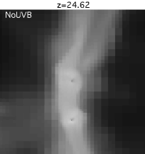
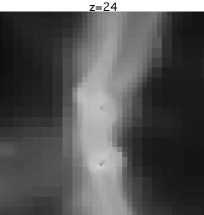
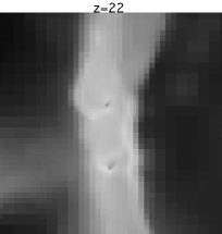
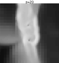
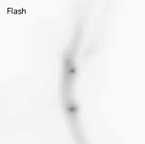
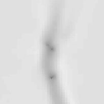
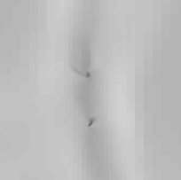
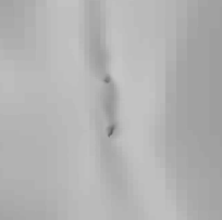
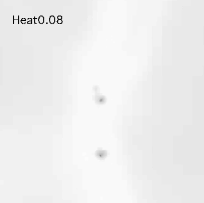
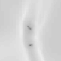
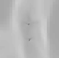
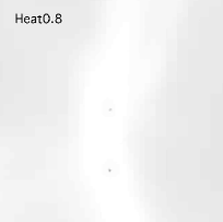
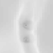
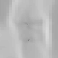
Figure 1.— Temperature projections of a 20 $h^{-1}$ kpc comoving region surrounding two halos nested in a filament. The rows, from top to bottom, correspond to the NoUVB, Flash, Heat0.08, and Heat0.8 runs. The columns, from left to right, correspond to redshifts of $z=$ 24.62, 24, 22, and 20. The scale is logarithmic, with black corresponding to $T<100$K and white corresponding to $T=10^{4}$ K.

In Figure 1, we show grey scale temperature projections of a 20 $h^{-1}$ kpc comoving region surrounding two halos nested in a filament. The rows correspond to the NoUVB, Flash, Heat0.08, and Heat0.8 runs (from top to bottom). The columns correspond to redshifts $z=$ 24.62, 24, 22, and 20 (from left to right). The scale is logarithmic, with black corresponding to $T<100$K and white corresponding to $T=10^{4}$K. The halo in the lower (upper) part of each figure grows from $M=7.2\times 10^{5}M_{\odot}$ ($M=6.9\times 10^{5}M_{\odot}$) at $z=24.62$ to $M=1.4\times 10^{6}M_{\odot}$ ($M=1.2\times 10^{6}M_{\odot}$) at $z=20$, as measured in the NoUVB run.

As one would expect, when the UVB is turned on, the gas is quickly ionized and heated. Gas which was previously at or close to hydrostatic equilibrium now has a greatly increased pressure gradient due to the increase in temperature. As a result, an outward–moving shock is formed, as clearly seen in Figure 1 for the last two rows (i.e. the runs which include a UVB with dynamical heating). Note that this shock is nearly absent in the Flash run. Subsequently, the gas in the dense filaments inside the shock is able to cool through Compton and H₂ cooling, and the shock stalls. The gas surrounding the halo starts infalling again. We explore these processes more quantitatively in § 3.1.

Note that the cores of the halos retain CD gas in all of the runs. In runs containing a UVB, the low density IGM outside of the filament still hasn’t cooled below $T\sim 10^{3}$K by $z=20$; however, the filament itself shows evidence of positive feedback in the Flash and Heat0.08 runs, with lower temperatures at $z\mathrel{\hbox to0.0pt{\lower 4.0pt\hbox{\hskip 1.0pt$\sim$}\hss}\raise 1.0pt\hbox{$<$}}24$ than in the NoUVB run. Furthermore, it is evident that once the UVB is turned off, the dense filament is able to cool very rapidly, from $T\sim 10^{4}$K to $T\sim 10^{3}$K in $\Delta z\mathrel{\hbox to0.0pt{\lower 4.0pt\hbox{\hskip 1.0pt$\sim$}\hss}\raise 1.0pt\hbox{$<$}}0.6$, due to the increased electron fraction, as we shall see below.

3.1. Halo Profiles

Figure 2.— Spherically averaged radial profiles of the same halo in the NoUVB (solid lines) and Heat0.8 (dashed lines) simulation runs. This halo was able to first form CD gas at $z=21$ ($z=18$) in the NoUVB (Heat0.8) run, respectively. The left pair of figures show a snapshot at $z=z_{\rm UVB,off}=24.62$, the middle pair at $z=23$, and the right pair at $z=18$. The virial radius of the halo increases from $R_{\rm vir}\sim 100$ pc at $z=24.62$, to $R_{\rm vir}\sim 200$ pc at $z=18$. All quantities are shown in proper (not comoving) units. The Upper panels show the hydrogen density, mass-weighted gas temperature, gas cooling time, and radial velocity (clockwise from upper left). The Bottom panels show mass fractions of HI, HII, H₂, and the number fraction of $e^{-}$ (clockwise from upper left).

To get a more quantitative idea of the feedback introduced by a UVB, in Figure 2 we plot spherically averaged radial profiles for the same individual halo at redshifts $z=$ 24.62, 23, and 18 (left to right), and in two different runs: NoUVB and Heat0.8 (solid and dashed lines, respectively). Figures in the top row show hydrogen density, mass-weighted gas temperature, gas cooling time, and radial velocity (clockwise from upper left). Figures in the bottom row shows mass fractions of HI, HII, H₂, and the number fraction of $e^{-}$ (more precisely, $f_{e}$ is defined as the mass fraction of $e^{-}$, normalized such that each $e^{-}$ is assumed to have the mass of hydrogen) (clockwise from upper left). The halo has a mass of M($z=24.62$) = $3.42\times 10^{5}M_{\odot}$ and M($z=18$) = $2.37\times 10^{6}M_{\odot}$ [taken from the NoUVB run; note that the mass in the Heat0.8 run is somewhat smaller, e.g., M($z=18$) = $2.24\times 10^{6}M_{\odot}$, due to photo-evaporation and a slight suppression of gas accretion as a result of the UVB].

From the profiles, one can see the impact of photo-evaporation in the Heat0.8 simulation run: the radially–outward moving shock mentioned above, as well as an accompanying decrease in density. As soon as the ionizing radiation is turned off, the gas cools from a temperature of $\sim 10^{4}$ K to $\sim 10^{3}$ K quite rapidly, with the free electron number fraction (approximately corresponding to the bottom left panels of the bottom row of Fig. 2), dropping two orders of magnitude by $z=23$, $\Delta z=1.62$, since the UVB was turned off. Also, the shock starts to dissipate by $z\sim 23$, with most of the gas switching to the infall regime again. Despite the evident photo-evaporation, the presence of the UVB has caused over an order of magnitude increase in the H₂ fraction, due to the increased (out–of–equilibrium) number of free electrons soon after $z_{\rm UVB,off}$.

We note that this halo managed to first form CD gas at $z=21$ in the NoUVB case, but the formation of CD gas was delayed in the Heat0.8 case until $z=18$. This delay can be crudely understood by looking at three fundamental time-scales: the H₂ cooling time,

$$t_{\rm H_{2}}=\frac{1.5k_{B}T}{\Lambda_{\rm H_{2}}}\frac{n_{g}}{n_{\rm HI}n_{\rm H_{2}}}~{},$$ (1)

the Compton cooling time,

$$t_{\rm C}\approx 14\left(\frac{1+z}{20}\right)^{-4}x_{e}^{-1}~{}{\rm Myr}~{},$$ (2)

and the gas recombination time,

$$t_{\rm rec}\approx 39\left(\frac{1+z}{20}\right)^{-3}\delta^{-1}x_{e}^{-1}~{}{\rm Myr}~{}.$$ (3)

Here, $k_{B}$ is the Boltzmann constant, $T$ is the temperature, $\Lambda_{\rm H_{2}}$ is the H₂ cooling function, $x_{e}$ is the free electron number fraction, $n_{g}$, $n_{\rm HI}$, and $n_{\rm H_{2}}$ are the number densities of all baryons and electrons, neutral hydrogen, and H₂, respectively, and $\delta$ is the gas overdensity, $\delta\equiv n_{g}/\bar{n}_{g}-1$.

The first column of Figure 2 shows a snapshot of our halos immediately prior to turning off the UVB. Note that the cooling time in the Heat0.8 run is several orders of magnitude lower than in the NoUVB run. At large radii, this is due to Compton cooling, since the UVB dramatically increases $x_{e}$ and the Compton cooling time (eq. 2) scales as $x_{e}^{-1}$. Additionally, the temperature increase to $\sim 10^{4}$ K allows for far more efficient line cooling from atomic hydrogen than in the NoUVB case. We also see that the structure of halos is important in accurately predicting feedback. Specifically, we note that the central region can behave quite differently than the outer regions of the halo.

Initially, immediately after the radiation field is turned off, the gas cools due to atomic line cooling. However, this quickly becomes inefficient below temperature of about 6000 K. While the radiation is on, the H₂ abundance is highly suppressed due to Lyman-Werner dissociation. However, as the temperature drops, the amount of H₂ increases rapidly because of the high electron abundance. In fact the molecular hydrogen formation time is shorter than the recombination time and a large amount of molecular hydrogen is produced, $x_{\rm H_{2}}\sim 3\times 10^{-3}$, irrespective of the density and temperature (see the discussion in Oh & Haiman 2002 for an explanation of this freeze-out value).

Due to the relatively high densities throughout the halo ($\delta\sim 10^{4}$ near the core), as well as the high initial $x_{e}$, the majority of the hydrogen recombines shortly after $z_{\rm UVB,off}$ in the Heat0.8 case ($t_{\rm rec}(z_{\rm UVB,off})\ll 1$Myr). After a few recombination times, $n_{g}\sim n_{\rm HI}$, and so eq. (1) can be simplified to

$$t_{\rm H_{2}} \approx \frac{1.5kT}{\Lambda}\frac{1}{n_{g}x_{\rm H_{2}}}$$

$$\approx 4\left(\frac{T}{10^{3}K}\right)^{-2.5}\left(\frac{x_{\rm H_{2}}}{3\times 10^{-3}}\right)^{-1}\left(\frac{n_{g}}{1\rm cm^{-3}}\right)^{-1}{\rm Myr}~{},$$

where $x_{\rm H_{2}}$ is the number fraction of H₂. This highly efficient molecular cooling channel is largely responsible for quickly driving the temperature down to about 1000 K (although a persistent LW background can counter this ${\rm H_{2}}$–enhancement effect; see below). Hence, we note that the cooling times near the halo core are comparable for both runs at $z=23$, with the cooling time in the Heat0.8 case being larger by a factor of a few.

This factor of only a few change in the cooling time is due to the remarkable cancellation of two strong effects, and can be understood by noting that the UVB induced photo-evaporation reduces $n_{g}$ by a factor of $\sim 40$ near the core at $z=23$. Meanwhile, the UVB boosts $x_{\rm H_{2}}$ near the core by a factor of $\sim 10$. Since Compton cooling is ineffective at this stage, the cooling time is dominated by the H₂ cooling channel, whose cooling time roughly scales as $t_{\rm H_{2}}\propto(n_{g}x_{\rm H_{2}})^{-1}$, given that the temperature is almost identical near the core at $z\sim 23$, and that the cooling function is very weakly dependent on $n_{\rm H_{2}}$ in this regime (Galli & Palla, 1998).

From this crude estimate, one obtains an effective “delay” in the formation of CD gas in the Heat0.8 run with respect to the NoUVB run:

$$f_{\rm delay}\sim\frac{t_{\rm H_{2}}^{\rm Heat0.8}}{t_{\rm H_{2}}^{\rm NoUVB}}\sim\left(\frac{n^{\rm NoUVB}_{g}}{n^{\rm Heat0.8}_{g}}\right)\left(\frac{x^{\rm Heat0.8}_{\rm H_{2}}}{x^{\rm NoUVB}_{\rm H_{2}}}\right)^{-1}\sim\frac{40}{10}\sim 4.$$ (5)

This is in excellent agreement with the delay observed in the pair of simulation runs, where the halo obtains CD gas $\sim$ 20 (60) Myr after our data point at $z=23$ in the NoUVB (Heat0.8) case, yielding a delay of a factor of $f_{\rm delay}\sim 3$.

3.2. $H_{2}$ production

                                                                        

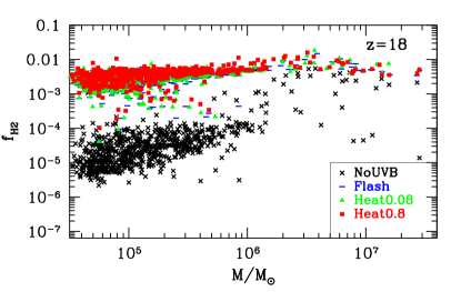
Figure 3.— Mass fractions of H₂ at $z=18$. Results are shown from the NoUVB (black crosses), Flash (blue dashes), Heat0.08 (green triangles), and Heat0.8 (red squares) simulation runs.

As mentioned above, molecular hydrogen can provide a dominant cooling mechanism, especially in high density regions. To study the impact of the UVB on the formation of H₂, we plot the H₂ mass fractions as functions of halo mass in Figure 3, at the lowest redshift of our simulations, $z=18$. Results are shown from the NoUVB (black crosses), Flash (blue dashes), Heat0.08 (green triangles), and Heat0.8 (red squares) simulation runs.

We note that in all of our runs which include a UVB, the molecular hydrogen fraction converges to a value which is nearly independent of the strength and duration of the UVB. As seen in Figure 3, by the end of our simulations, most halos which have been exposed to a UVB in their past have settled on a value of a few $\times 10^{-3}$ for the mass fraction of H₂. This freeze–out value is due to the fact that the number density of H₂ follows its equilibrium value until about 3000 K, below which recombination proceeds more quickly than H₂ formation and the fraction freezes out at this point (Oh & Haiman, 2002). This number is fairly independent of mass, though there is a weak trend towards higher mass fractions for higher mass halos, up to mass fractions of $\sim 10^{-2}$ for $M\sim 4\times 10^{6}M_{\odot}$. Note also that there is some evidence for a non-monotonic evolution of the H₂ fraction, with mass fractions falling back down to $\sim 4\times 10^{-3}$ by $M\sim 3\times 10^{7}M_{\odot}$.

In contrast, molecular hydrogen in halos which have not been exposed to a UVB (black crosses in Figure 3) is distinctly sparser (over two orders of magnitude for $M\mathrel{\hbox to0.0pt{\lower 4.0pt\hbox{\hskip 1.0pt$\sim$}\hss}\raise 1.0pt\hbox{$<$}}10^{6}M_{\odot}$) than in our other runs. Also, there is a stronger evolution with respect to mass, as well as more scatter (which makes sense, since the ${\rm H_{2}}$ abundance in this case is not a result of a freeze–out process, and depends strongly on local density and temperature).

An interesting conclusion can be drawn from the similarity of H₂ fractions in our runs which include a UVB. Namely, if our analysis of the dominant cooling processes in § 3.1 is accurate, the differences between the CD gas fractions among our UVB runs is predominately due to disparate effectiveness of photo-evaporation. In other words, as the positive feedback (i.e. the increase of the $x_{\rm H_{2}}$ term in eq. 3.1) is nearly independent of the strength and duration of the UVB in our runs, only the amount of negative feedback (decrease in $n_{g}$) causes variations in the delay in the formation of CD gas (see a more detailed discussion in § 4 below). We have also verified for several halos that this similarity in the total H₂ fraction extends to the radial profiles of H₂.

3.3. Ensemble Evolution of the Cold, Dense Gas Fractions

Figure 4.— Total gas fractions (top panels) and cold, dense gas fractions (bottom panels) as a function of total halo mass at redshift $z=18$, the lowest redshift output of our simulations. The four panels correspond to the NoUVB (top left), Flash (top right), Heat0.08 (bottom left), and Heat0.8 (bottom right) simulation runs.

As mentioned above, a quantity of particular importance in studying the capacity of a halo at hosting stars is its cold, dense (CD) gas fraction, $f_{\rm cd}$, defined above. Here we show the general trends for the evolution of this quantity for the population of halos in our simulations, as we vary the UVB.

In Figure 4, we plot the total gas fractions (upper panels) and CD fractions (lower panels) as a function of total halo mass at redshift $z=18$, the lowest redshift output of our simulations. The figures correspond to the NoUVB (top left), Flash (top right), Heat0.08 (bottom left), and Heat0.8 (bottom right) simulation runs.

Note that while the total gas fractions of small halos ($M\mathrel{\hbox to0.0pt{\lower 4.0pt\hbox{\hskip 1.0pt$\sim$}\hss}\raise 1.0pt\hbox{$<$}}$ few $\times 10^{5}M_{\odot}$) that have been exposed to a UVB are suppressed with respect to the NoUVB case, there is little immediate visual evidence of either negative or positive feedback for halos large enough to host CD gas ($M\mathrel{\hbox to0.0pt{\lower 4.0pt\hbox{\hskip 1.0pt$\sim$}\hss}\raise 1.0pt\hbox{$>$}}$ few $\times 10^{5}M_{\odot}$). The Flash CD gas fractions show evidence of positive feedback in the mass range $\sim~{}2\times 10^{5}$ – $10^{6}$ $M_{\odot}$, while the Heat0.8 run shows evidence of strong negative feedback in the same mass range, with no halos hosting CD gas at $M<10^{6}M_{\odot}$. These small halos are the ones which would be most affected by photo–evaporation. This lends further credibility to our assertion above that positive feedback in runs which include a UVB is fairly independent of the UVB strength, and hence the total feedback is set by photo–evaporation effects (i.e. negative feedback). The Heat0.08 run has a near zero balance of positive and negative feedback.

In order to better quantify the amount of suppression of CD gas in our models incorporating a UVB, as well as the evolution of such a suppression with redshift, we define the cumulative, fractional suppression of the halo number as

$$\delta_{N,{\rm cd}}(z)\equiv\frac{N_{\rm cd}^{{\rm run}i}(z)-N_{\rm cd}^{{\rm run}i}(z_{\rm UVB,on})}{N_{\rm cd}^{\rm NoUVB}(z)-N_{\rm cd}^{\rm NoUVB}(z_{\rm UVB,on})}-1~{},$$ (6)

where $N_{\rm cd}^{\rm NoUVB}(z)$ and $N_{\rm cd}^{{\rm run}i}(z)$ are the total number of halos with CD gas at redshift $z$ in the NoUVB run and some given run $i$, respectively. This expression is well–defined for $N_{\rm cd}^{\rm NoUVB}(z)$ $>$ $N_{\rm cd}^{\rm NoUVB}(z_{\rm UVB,on})$; for $N_{\rm cd}^{\rm NoUVB}(z)$ = $N_{\rm cd}^{\rm NoUVB}(z_{\rm UVB,on})$, we set $\delta_{N,{\rm cd}}(z)\equiv 0$. Note that by definition, $N_{\rm cd}^{\rm NoUVB}(z_{\rm UVB,on})$ = $N_{\rm cd}^{{\rm run}i}(z_{\rm UVB,on})$.

Similarly, we define the cumulative, fractional suppression of the CD gas mass as

$$\delta_{M,{\rm cd}}(z)\equiv\frac{M_{\rm cd}^{{\rm run}i}(z)-M_{\rm cd}^{{\rm run}i}(z_{\rm UVB,on})}{M_{\rm cd}^{\rm NoUVB}(z)-M_{\rm cd}^{\rm NoUVB}(z_{\rm UVB,on})}-1~{},$$ (7)

where $M_{\rm cd}^{\rm NoUVB}(z)$ and $M_{\rm cd}^{{\rm run}i}(z)$ are the total mass of CD gas at redshift $z$ in the NoUVB run and some given run $i$, respectively. The total CD gas mass is obtained by merely summing the CD gas masses for all of the halos in the simulation. As for equation (6), this expression is well–defined for $M_{\rm cd}^{\rm NoUVB}(z)$ $>$ $M_{\rm cd}^{\rm NoUVB}(z_{\rm UVB,on})$, and for $M_{\rm cd}^{\rm NoUVB}(z)$ = $M_{\rm cd}^{\rm NoUVB}(z_{\rm UVB,on})$, we set $\delta_{M,{\rm cd}}(z)\equiv 0$.

                                                                        

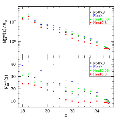
Figure 5.— Values of $M_{\rm cd}^{{\rm run}i}(z)$ (top panel) and $N_{\rm cd}^{{\rm run}i}(z)$ (bottom panel) as defined in equations (7) and (6). The results are displayed for the NoUVB (crosses), Flash (dashes), Heat0.08 (triangles), and Heat0.8 (squares) simulation runs.

Equations (6) and (7) provide an estimate of how the CD gas has been affected by the presence of a UVB, following the turn-on redshift of the UVB, $z_{\rm UVB,on}$ (the values at $z_{\rm UVB,on}$ are subtracted in order to provide a more sensitive measure of relative changes of CD gas). As defined above, $\delta_{N,{\rm cd}}(z)=0$ and $\delta_{M,{\rm cd}}(z)=0$ if the UVB has no effect. If the effect of a UVB is positive, resulting in positive feedback, $\delta_{N,{\rm cd}}(z)$ and $\delta_{M,{\rm cd}}(z)$ would be positive. If the effect of the UVB is negative, $\delta_{N,{\rm cd}}(z)$ and $\delta_{M,{\rm cd}}(z)$ would be negative.

In Figure 5, we plot the values of $M_{\rm cd}^{{\rm run}i}(z)$ (top panel) and $N_{\rm cd}^{{\rm run}i}(z)$ (bottom panel) in our four main simulation runs: ${\rm run}i$ = NoUVB (crosses), Flash (dashes), Heat0.08 (triangles), and Heat0.8 (squares). The corresponding values of $\delta_{M,{\rm cd}}(z)$ and $\delta_{N,{\rm cd}}(z)$ are plotted in Figure 6 in the top and bottom panels, respectively. The results are displayed for the Flash (dashes), Heat0.08 (triangles), and Heat0.8 (squares) simulation runs. Although some of the notable fractional changes shown in Figure 6 might appear statistically insignificant due to the small number statistics inferred from Figure 5, it should be noted that these runs are not uncorrelated experiments. In other words, each of our runs in Table 1 is seeded with the same initial conditions, and so small relative changes compared to the NoUVB run are significant (i.e. the errors are not Poisson).

One can infer from Figures 5 and 6 that the Heat0.8 run shows evidence of strong negative feedback down to $z\sim 20$, with values approaching the NoUVB run by the end of our simulation ($z=18$). Conversely, the Flash run exhibits strong positive feedback down to $z\sim 20$, and again approaches the NoUVB run by the end of our simulation. In the middle is the Heat0.08 run, which shows very little difference compared to the NoUVB run (initially there is some evidence of mild positive feedback down to a redshift of $z=21$, but at redshifts below that, little evidence remains of a UVB ever being present).

It is also interesting to note that while the halo number in the Heat0.8 run shows negative feedback down to $z=18$ (bottom panels of Figures 5 and 6), the total mass of CD gas (top panels of Figures 5 and 6) shows no such feedback at $z\mathrel{\hbox to0.0pt{\lower 4.0pt\hbox{\hskip 1.0pt$\sim$}\hss}\raise 1.0pt\hbox{$<$}}19$. The explanation for this apparent contradiction is that the total mass of CD gas is dominated by the largest halos (both because these halos are more massive and because the fraction of CD gas increases with mass), and as Figure 4 shows, these large halos are largely unaffected by the ionizing radiation. Conversely, the elimination of the CD gas from the lowest–mass halos even at $z=18$ is a genuine effect (as is clearly visible in the lower right panel in Fig 4), but these halos do not contribute significantly to the total CD mass summed over all halos.

Figure 6 agrees well with the qualitative inferences drawn above. Furthermore, it explicitly shows that the critical UVB flux cutoff in our simulation between inducing a net negative and net positive feedback is $J_{\rm UV}\sim 0.1$. Halos which have been exposed to a fainter UVB exhibit positive feedback, whereas halos which have been exposed to a brighter UVB exhibit negative feedback. However, it is also important to note that any such feedback is temporary, as all of our runs begin to converge by the end of our simulations at $z=18$. The exception is that the Heat0.8 run shows persistent suppression of the smallest halos (with $M<10^{6}M_{\odot}$) all the way down to $z=18$.

                                                                        

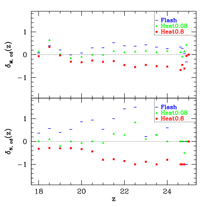
Figure 6.— Values of $\delta_{M,{\rm cd}}(z)$ (top panel) and $\delta_{N,{\rm cd}}(z)$ (bottom panel) as defined in equations (7) and (6). The results are derived from Figure 5 and displayed for the Flash (dashes), Heat0.08 (triangles), and Heat0.8 (squares) simulation runs.

3.4. Relating initial densities at $z_{\rm UVB,on}$ to subsequent suppression of cold, dense gas

Here we attempt to generalize and physically motivate some of the results from the previous section. In particular, we have already seen that feedback depends on $J_{\rm UV}$ and $M_{\rm halo}$. Here we examine whether a halo’s capacity for forming CD gas depends strongly on the properties of its progenitor region at the time of the UV–illumination ($z_{\rm UVB,on}$). Specifically, we expect those progenitor regions which are less dense at $z_{\rm UVB,on}$, and hence at an earlier evolutionary stage, to be more susceptible to negative photo–heating and photo–evaporation feedback than more dense regions. This is because the ${\rm H_{2}}$ photo–dissociation rate scales with the density, whereas ${\rm H_{2}}$–forming reaction rates scale with the square of the density; as a result, photo–dissociation becomes comparatively more important at low densities (Oh & Haiman, 2003). Below we focus on the Heat0.8 run, as it exhibits the strongest negative feedback.

We divide the set of halos with CD gas at redshift $z$ in our NoUVB run into two groups: those that also have CD gas in the Heat0.8 run (group 1), and those that do not also have CD gas in the Heat0.8 run (group 2). From Figure 4, one can note that at $z=18$ it is possible to define a rough mass scale that separates these two groups; namely halos with masses $\mathrel{\hbox to0.0pt{\lower 4.0pt\hbox{\hskip 1.0pt$\sim$}\hss}\raise 1.0pt\hbox{$>$}}10^{6}M_{\odot}$ do not have their CD gas suppressed (group 1), and halos with masses $\mathrel{\hbox to0.0pt{\lower 4.0pt\hbox{\hskip 1.0pt$\sim$}\hss}\raise 1.0pt\hbox{$<$}}10^{6}M_{\odot}$ do have their CD gas suppressed (group 2). As stated above, we hypothesize that the physical distinction between the two sets occurs due to their differences at the redshift they were exposed to the UVB, $z_{\rm UVB,on}$. Specifically, we compare the mass-weighted, average densities of progenitor regions at $z_{\rm UVB,on}$ = 25, which are to become our halos from groups 1 or 2 at some later $z$. We do this by tracing back all dark matter particles comprising each halo at $z$ to their positions at $z=z_{\rm UVB,on}$, and then obtaining the average gas density at that position.

As there are too few halos to accurately construct the group 1 and group 2 mean density distribution functions (see bottom panel of Fig. 5), we present their properties via a density cutoff. We adopt a simple criterion to define a density cutoff, $\rho_{\rm cutoff}$, between the two groups. We chose $\rho_{\rm cutoff}$ so that the sum of the fraction of group (1) points below $\rho_{\rm cutoff}$ and the fraction of group (2) points above $\rho_{\rm cutoff}$ is minimized. Specifically, this fractional sum used as a proxy for the disjointness of the two distributions is defined as

$$f_{\rm fit}\equiv{\rm MIN}\left[f_{1}(<\rho_{\rm cutoff})+f_{2}(>\rho_{\rm cutoff})\right]$$ (8)

where $f_{1}(<\rho_{\rm cutoff})$ is the fraction of halos in group 1 which have mean densities less than the cutoff density, and $f_{2}(>\rho_{\rm cutoff})$ is the fraction of halos in group 1 which have mean densities greater than the cutoff density. In essence, each term is the fraction of “misclassified” halos, and so we want to select $\rho_{\rm cutoff}$ such that $f_{\rm fit}$ is minimized. The sum as defined in equation (8) ranges from 0 to 2, while our figure of merit ranges from $f_{\rm fit}=0$ for two completely disjoint distributions to $f_{\rm fit}=1$ for the case where group 1 and group 2 are drawn from the same underlying distribution (not taking into account Poisson errors).

We plot values for the density cutoff (in units of the average comoving density, $\bar{\rho}$) as a function of redshift in the top panel of Figure 7. Our disjointness figure of merit is plotted in the bottom panel of Figure 7. Note that for most redshifts, $f_{\rm fit}\ll 1$, meaning that the group 1 and group 2 density distributions are quite disjoint, and that the density cutoff, $\rho_{\rm cutoff}$, has a well-defined value. One can get a sense of the Poissonian errors associated with $\rho_{\rm cutoff}$ by looking at the bottom panel of Figure 5, since ${\rm N_{group1}}\sim N_{\rm cd}^{\rm Heat0.8}\sim 10-20$ and ${\rm N_{group2}}\sim N_{\rm cd}^{\rm NoUVB}-N_{\rm cd}^{\rm Heat0.8}\sim 10$. One should also note that $f_{\rm fit}$ increases with decreasing $\rho_{\rm cutoff}$, which is to be expected as the density distributions can not have negative values, so both distributions start being “packed” together as they approach zero. In other words, there is an intrinsic “noise” consisting of small environmental fluctuations (halo location, peculiar velocity, etc.), and this noise becomes more noticeable as $\rho_{\rm cutoff}\rightarrow 0$. In practice, it is difficult to disentangle this effect from an actual merging of the two distributions.

As expected, halos with less dense progenitor regions at $z_{\rm UVB,on}$ are more susceptible to negative feedback. It is quite interesting to note that our density cutoff decreases exponentially with redshift, implying that an increasing fraction of the photo–heated mass will fall in the “borderline” region between negative and positive feedback. This provides further support for our earlier claim that the fossil HII region “forgets” the UVB as time passes. In other words, a strong UVB serves to merely delay the gas from cooling and collapsing; the gas eventually manages to cool, aided by an enhanced $\rm H_{2}$ fraction and enhanced infall (see Figure 2, and associated discussion). The length of this delay is a strong function of the density of halo progenitor regions at $z_{\rm UVB,on}$, as one would expect from our analysis in § 3.1.

                                                                        

Figure 7.— The critical density $\rho_{\rm cutoff}$, upper panel, for the progenitor gas at $z_{\rm UVB,on}$ = 25 of halos that collapse at some later redshift $z$, roughly divides halos experiencing negative vs. positive feedback at redshift $z$ (i.e. halos that were more/less dense than $\rho_{\rm cutoff}$ at the time of illumination will experience positive/negative feedback). $\rho_{\rm cutoff}$ is a mass-weighted mean density of the progenitors pieces of the halo, shown in units of the average comoving density, $\bar{\rho}$ in our Heat0.8 run. The values of $f_{\rm fit}$, shown in the Lower panel, show a rough figure of merit for how well the fixed density $\rho_{\rm cutoff}$ separates halos into two disjoint categories ($f_{\rm fit}\ll 1$ indicates a clear separation). See text and equation (8) for definitions and discussion.

It is numerically impractical to run our simulations to redshifts much lower than $z\mathrel{\hbox to0.0pt{\lower 4.0pt\hbox{\hskip 1.0pt$\sim$}\hss}\raise 1.0pt\hbox{$<$}}18$, due to the rapidly increasing collapsed fraction in our refined region (see Fig. 17). On the other hand, it would be interesting to know what eventually happens to most of the mass of our refined region. A step towards answering this question is to find out whether the majority of the mass of our refined region at $z=z_{\rm UVB,on}$ is located in overdensities below or above the lowest redshift $\rho_{\rm cutoff}$ value shown in Figure 7. With this motivation, we obtained a mass-weighted density distribution over randomly generated positions inside our refined region. We select a radius surrounding each position, such that a given number of DM particles lie within that radius (the number of particles is chosen to correspond to the halo masses capable of hosting CD gas). We then obtain a mass-weighted average density by averaging over the gas densities at the location of each DM particle inside our chosen radius.

                                                                        

Figure 8.— Mass-weighted, cumulative density distributions for regions of $M\sim 8.9\times 10^{5}M_{\odot}$ (solid curves) and $M\sim 8.9\times 10^{6}M_{\odot}$ (dashed curves). Two redshift values are presented: $z_{\rm UVB,on}$ = 33 and 25, from left to right. Note that $\rho$ is the comoving gas density.

In Figure 8, we plot the cumulative density distributions (fraction of regions with mass-weighted density less than $\rho$) thus generated at $z$ = 33 and 25, from left to right, and for regions of mass scale $M\sim 8.9\times 10^{5}M_{\odot}$ ($\sim 10^{3}$ DM particles) and $M\sim 8.9\times 10^{6}M_{\odot}$ ($\sim 10^{4}$ DM particles) with solid and dashed lines, respectively. Understandably, the larger mass scales shift the mean density towards larger values, due to the increased likelihood of averaging over dense patches. Also, we see that for regions of equal mass scales, the higher redshift counterparts have a lower mean density, partly due to a smaller clumping factor and partly due to to the fact that we plot comoving density, which increases with decreasing redshift.

Figure 8 shows that the majority of the mass ($\mathrel{\hbox to0.0pt{\lower 4.0pt\hbox{\hskip 1.0pt$\sim$}\hss}\raise 1.0pt\hbox{$>$}}90\%$) of our refined region is located in regions with mean densities lower than $\sim 10\bar{\rho}$, the lowest cutoff obtained by our analysis (see Figure 7). Hence, we cannot rule out the possibility of significant negative feedback at lower redshifts, not probed by our simulation. Nevertheless, we regard this as unlikely, for two reasons. First, halos will be centered around overdensities, not random points, and subsequent growth of the halo’s mass need not be spherically symmetric; these effects will bias the relevant density distribution to higher values than shown in Figure 8. Second, it is likely that most halos massive enough to host CD gas, which form in our biased region at $z<18$, already had a dense progenitor core at $z=z_{\rm UVB,on}$. Indeed, we find that all halos hosting CD gas at $z=18$ in the NoUVB run had some dense progenitor gas ($\rho\mathrel{\hbox to0.0pt{\lower 4.0pt\hbox{\hskip 1.0pt$\sim$}\hss}\raise 1.0pt\hbox{$>$}}100\bar{\rho}$) at $z_{\rm UVB,on}=25$. Subsequent growth could be dominated by gas accretion onto these dense regions, and merging with other halos (rather than forming fresh halos entirely from low–density gas). Nevertheless, we emphasize that we chose to simulate a biased volume (favoring early collapse), and the above arguments will be less valid in a more typical patch of the IGM (with lower densities).

3.5. Early UVB Run

Ideally, one would want to explore all of parameter space by varying $J_{\rm UV}$, $z_{\rm UVB,on}$ and $z_{\rm UVB,off}$, with different realizations of the density field. Unfortunately, given computational limitations, this is impossible. However, in order to confirm the trends we present above, we run another simulation, EarlyHeat0.8, in which we turn on a UVB, with an amplitude of $J_{\rm UV}=0.8$, at $z_{\rm UVB,on}=33$, and turn it off at $z_{\rm UVB,off}=32.23$. We then repeat the analysis in § 3.4. The corresponding figures, Figures 9 and 10, are presented below.

Figure 10 shows that we once again find strong negative feedback down to $z\sim 23$. For $z<23$, we see virtually no evidence of any feedback, lending further credibility to our interpretation above, that our other runs “forget” the episode of UV heating, and start converging to the NoUVB run by the end of our simulations ($z=18$).

                                                                        

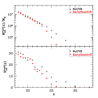
Figure 9.— Values of $M_{\rm cd}^{{\rm run}i}(z)$ (top panel) and $N_{\rm cd}^{{\rm run}i}(z)$ (bottom panel) as defined in equations (7) and (6). The results are displayed for the NoUVB (crosses) and EarlyHeat0.8 (squares) simulation runs.

                                                                        

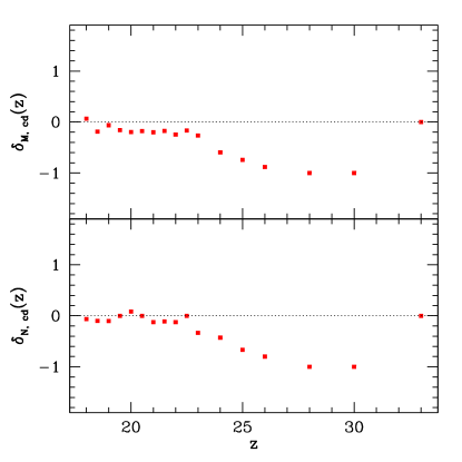
Figure 10.— Values of $\delta_{M,{\rm cd}}(z)$ (top panel) and $\delta_{N,{\rm cd}}(z)$ (bottom panel) as defined in equations (7) and (6), shown here in the EarlyHeat0.8 run.

In Figure 11, we plot the density cutoff, $\rho_{\rm cutoff}$, defined in § 3.4, for both the Heat0.8 (crosses) and EarlyHeat0.8 (triangles) runs. For the sake of a direct comparison, this time we use physical units both for $\rho_{\rm cutoff}$, (proper cm^-3), and for the time elapsed since the UVB turn-off (Myr). Unfortunately, the drawback to having a simulation run with such an early heating episode is that there are fewer halos to analyze at earlier epochs. Specifically, in the epoch with evident negative feedback ($z\mathrel{\hbox to0.0pt{\lower 4.0pt\hbox{\hskip 1.0pt$\sim$}\hss}\raise 1.0pt\hbox{$>$}}23$), as seen below, there are only three redshift outputs containing both halos exhibiting suppression and halos not exhibiting suppression of CD gas (groups 2 and 1, respectively, defined in § 3.4). While it is difficult to draw strong conclusions from Figure 11, the density cutoff values do appear similar in the two runs.

We examined the radial profiles of the same halo pictured in Figure 2, to verify that we can apply the same cooling arguments as discussed in § 3.1. We compare the NoUVB and EarlyHeat0.8 runs at $z=30$, shortly after $z_{\rm UVB,off}=33$. As in Figure 2, this redshift corresponds roughly to the regime where the induced shock begins to dissipate, and the gas starts falling back into the core. In all of the runs, the temperature drops to $T\sim T_{\rm vir}\sim 10^{3}$K near the core very soon after $z_{\rm UVB,off}$. As in § 3.1, we characterize the delay in formation of CD gas with (c.f. eq. (5))

$$f_{\rm delay}\sim\left(\frac{n^{\rm NoUVB}_{g}}{n^{\rm Heat0.8}_{g}}\right)\left(\frac{x^{\rm Heat0.8}_{\rm H_{2}}}{x^{\rm NoUVB}_{\rm H_{2}}}\right)^{-1}\sim\frac{25}{20}\sim 1.$$ (9)

From our simple cooling argument, we predict a nearly negligible delay for this halo. Indeed, the halo ends up forming CD gas at $z=20.5$ in the EarlyHeat0.8 run, and at $z=21$ in the NoUVBrun, showing a very small delay.

Despite the halo’s exposure to the UVB earlier in its evolution and subsequent lower gas density, the total negative feedback is reduced compared to the Heat0.8 run. Compared to the Heat0.8 run, the negative feedback, when expressed as the photo-evaporation term in the above equation $(n^{\rm NoUVB}_{g}/n^{\rm Heat0.8}_{g})$ is smaller by a factor of $\sim 2$, and the positive feedback, when expresses as the H₂ fraction term in the above equation $(x^{\rm Heat0.8}_{\rm H_{2}}/x^{\rm NoUVB}_{\rm H_{2}})$ is larger by a factor of $\sim 2$. These changes are explained by more efficient Compton cooling (which more effectively eliminates the impact of the photo–heating), and the lower gas density (which leads to a lower value for the ${\rm H_{2}}$ fraction in the NoUVB run, and hence a larger relative enhancement in the Heat0.8 run), respectively (Oh & Haiman, 2003).

                                                                        

Figure 11.— Values of $\rho_{\rm cutoff}$ (in proper cm^-3) as a function of time elapsed since $z_{\rm UVB,off}$. Crosses correspond to our Heat0.8 run (i.e. $z_{\rm UVB,on}=25$); triangles correspond to our EarlyHeat0.8 run (i.e. $z_{\rm UVB,on}=33$).

3.6. The impact of not including radiative transfer

Our simulations treat photo-ionization in the optically thin limit and so do not include radiative transfer effects. This results in two differences compared to a self-consistent treatment.

The most obvious effect is that all of our halos are ionized simultaneously, while in reality halos are ionized by very nearby stars with distances less than the few kpc radius of typical HII regions (Whalen et al., 2004; Kitayama et al., 2004). Nevertheless, we argue that the primary effect of this is to vary the flux felt by the halo and we explore a range of reasonable fluxes in our simulations. The exception is if the halo is so close that it is enveloped within the shock generated by the gas expelled from the halo hosting the star that produces the ionizing radiation. However, typically this shocked region occupies a volume of less than 1% of the ionized region (e.g., Whalen et al. 2004).

The second, and more important, effect of radiative transfer will be to shield the high density cores of our minihalos. If the cores are not ionized, then both the positive and negative feedback effect will clearly not occur in the neutral gas. Alvarez et al. (2006) estimate that self-shielding will set in at densities around a few particles per cm^-3 (depending on the strength of the flux and the size of the halo). This value is approximately the density we find in the cores of our simulated halos (e.g., Figure 2), and so we conclude that radiative transfer effects may play an important role in the cores of our halos. We note that at these densities, we typically find very little negative feedback anyway because of the short cooling times in the ionized gas. Most of the negative feedback we observe arises due to the photo-heating of low-density gas which is then later accreted onto halos. This means that we do not expect our results to be strongly affected by the missing radiative transfer effects. The effect, where important, will be to decrease the amount of feedback, making our statements about feedback upper limits on the amplitude of the expected feedback. Finally we note that, given time, the halos will be evaporated and eventually ionized despite the high densities in the core; however, this photo-evaporation time will be typically longer than 3 Myr (Haiman et al., 2001; Shapiro et al., 2004; Iliev et al., 2005).

4. The Impact of a Lyman Werner Background

While up to now we have ignored a possible Lyman–Werner background, such a background is likely to be present early on, and could have a strong impact on the ${\rm H_{2}}$ chemistry and gas cooling. In particular, the IGM is nearly optically thin, or quickly becomes so, at frequencies below 13.6eV (Haiman et al., 2000). For reference, we note that one photon per hydrogen atom (the minimum UV background required for reionizing the IGM) would translate to a background intensity of $J_{\rm LW}\sim 20[(1+z)/21]^{3}$. Background levels 2–4 orders of magnitude below this value will be established well before reionization, and have the potential to already photodissociate ${\rm H_{2}}$ molecules at these early epochs (Haiman et al., 1997; Machacek et al., 2001). Furthermore, and of more direct interest in the present study, Oh & Haiman (2003) have argued that the presence of an entropy floor, generated by the UV heating, reduces gas densities, and makes the ${\rm H_{2}}$ molecules in collapsing halos more vulnerable to a LW background. Motivated by the above, in this section, we study the impact of a LW background on our results. We start by a brief discussion of our results without a LW background (§ 4.1), use these results to build up some expectations for the impact of the LW background (§ 4.2), and then present the results of simulation runs with LW backgrounds (§ 4.3).

                                                                        

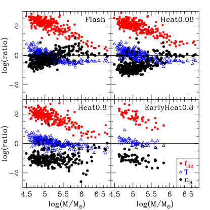
Figure 12.— The figure illustrates the impact of the UV heating in the four different runs (Flash, Heat0.08, Heat0.8, EarlyHeat0.8, as labeled in each panel). For each halo, we show, at $z=23$ (or $z=30$, in the early heating run), the ratio of the ${\rm H_{2}}$ fractions (red filled squares), the temperatures (blue empty triangle) and of the average gas density within the central 15pc (red filled circles) in the runs with UV heating, compared to the runs with no UVB. Note that the ${\rm H_{2}}$ fraction tends to increase by the same factor, regardless of the nature of the heating. As a result, the sign of the overall feedback (negative or positive) is determined primarily by the changes in the gas density, which does depend strongly on the type and amount of heating.

4.1. Discussion of Results without the LW Background

As already discussed above, the UV heating produces two prominent effects: it boosts the ${\rm H_{2}}$ fraction and it decreases the gas density. In the case of the individual halo studied in Figure 2 and described in § 3.1, and also in the case of the analogous halo in the early heating run, described in § 3.5 above, we have seen that the overall impact of the UV heating is a delay in the development of cold dense gas; this delay can be understood by the increase in the cooling time, given by the product of the two effects above.

In order to understand the net effect of the UV heating on the overall halo population, in Figure 12, we show the ratio of the ${\rm H_{2}}$ fractions (red filled squares), of the temperatures (blue empty triangle) and of the mean gas density within the central 15pc (red filled circles) in all four of our runs with UV heating. Each quantity is computed for every halo present at $z=23$ (or at $z=30$ in the early heating run), in the runs with UV heating, and the ratio refers to this value, divided by the same quantity in the run without a UV background.

The figure clearly shows that the ${\rm H_{2}}$ fractions are enhanced in a similar fashion in all of the runs (by factors ranging from several hundred at low mass, to a few at high mass). This is indeed expected: while the H₂ abundance is nearly independent of halo mass in runs with a UVB, it is a strongly increasing function of mass in the NoUVB case (see Figure 3). Because the “freeze–out” value of the ${\rm H_{2}}$ abundance, $f_{\rm H_{2}}\approx 2\times 10^{-3}$ is insensitive to the background flux or duration, or to the gas density (Oh & Haiman, 2002), the enhancement factor over the NoUVB run is always the same.

Contrary to the “universal” effect on the ${\rm H_{2}}$ fraction, the impact of the UV background on the gas density depends strongly on the nature of the heating. Not surprisingly, the flash heating case shows the weakest gas dilution; heating the gas for an extended period, at increasing flux levels, causes larger dilutions. Note that the impact on the density tends to diminish for more massive halos. This is partly because a fixed amount of heating/energy input corresponds to a smaller fraction of the halo’s total binding energy. In addition, the ${\rm H_{2}}$–cooling time is shorter than $10^{7}$ years in halos with $M\mathrel{\hbox to0.0pt{\lower 4.0pt\hbox{\hskip 1.0pt$\sim$}\hss}\raise 1.0pt\hbox{$>$}}10^{5.8}~{}{\rm M_{\odot}}$ and the UV–heated gas is able to cool prior to $z=23$. This latter effect is also directly evident in the gas temperature ratios, which decrease towards larger halos (and decrease below unity).

The above trends account for the basic results shown in Figure 6. Note that this figure shows only those halos that develop cold dense gas; i.e. those with $M\mathrel{\hbox to0.0pt{\lower 4.0pt\hbox{\hskip 1.0pt$\sim$}\hss}\raise 1.0pt\hbox{$>$}}10^{5.5}~{}{\rm M_{\odot}}$. In the Flash–ionization case, the ${\rm H_{2}}$ fraction enhancement in these halos dominates, and results in a positive overall feedback. In the Heat0.08 case, the effects on the ${\rm H_{2}}$ fraction and on the gas density nearly cancel each other and the net result is that the UV heating has almost no impact. In the Heat0.8 case, the dilution of the gas density dominates, and results in a delay in the cooling time, and in the development of the cold dense gas, by a factor of $1-10$.

4.2. The Impact of a Lyman Werner Background - Expectations

The above trends suggest that the UV heating can render the halos more susceptible to the negative effect of a LW background. As argued in Oh & Haiman (2003), the ${\rm H_{2}}$ photodissociation rate depends linearly on the gas density, while the rate of ${\rm H_{2}}$–forming two–body collisions scales with the square of the density; hence density dilution makes ${\rm H_{2}}$ photodissociation comparatively more important.

In order to investigate the impact of a LW background on the amount of cold dense gas, we performed a set of six additional simulation runs. Before describing these runs, however, we use the no–LW runs with UV heating (Heat0.8) and without heating to develop some expectations. These are shown in Figures 13–15, as follows.

                                                                        

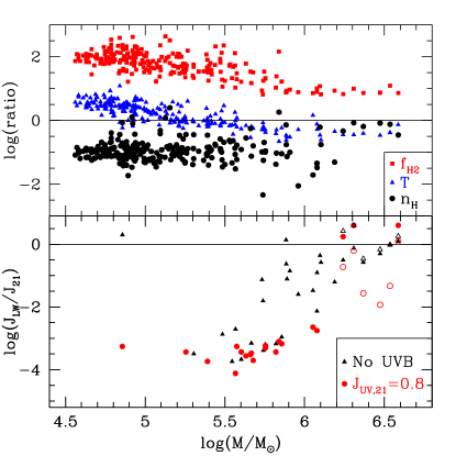
Figure 13.— Upper panel: The ratio of the ${\rm H_{2}}$ fractions, temperatures, and average gas density between the Heat0.8 and NoUVB runs, at $z=24$ (following the notation in Figure 12). Lower panel: The critical value of the background LW flux, $J_{\rm LW}$ (in units of $10^{-21}{\rm ergs~{}s^{-1}~{}cm^{-2}~{}Hz^{-1}~{}sr^{-1}}$) such that the gas temperature cools to $300$K by redshift $z=18$. Only those halos whose gas manages to cool by $z=18$ are shown. Values for the NoUVB run are represented by filled black triangles; values for the Heat0.8 run are represented by filled red circles. Empty symbols denote the critical value of $J_{\rm LW}$, such that the gas temperature decreases by half between redshifts $z=24$ and $z=18$ (see discussion in text).

                                                                        

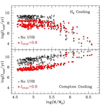
Figure 14.— Upper panel: ${\rm H_{2}}$–cooling time for each halo in the Heat0.8 (red, filled circles) and NoUVB (black, empty triangles) runs, at redshift $z=24$. Lower panel: Compton–cooling timescale for the same halos. Note that the ${\rm H_{2}}$–cooling time is shorter than the Hubble time in halos with $M\mathrel{\hbox to0.0pt{\lower 4.0pt\hbox{\hskip 1.0pt$\sim$}\hss}\raise 1.0pt\hbox{$>$}}10^{5.5}~{}{\rm M_{\odot}}$.

In Figure 13, in the upper panel, we show the ratio of the ${\rm H_{2}}$ fractions (red filled squares), of the temperatures (blue empty triangles) and of the mean gas density within the central 15pc (red filled circles). The ratios are computed in the Heat0.8 and NoUVB runs, as in Figure 12, but we here use $z=24$, rather than $z=23$. This choice is made to allow for some Compton cooling, but to minimize the ${\rm H_{2}}$–cooling that occurs after the heating is turned off (the latter may not occur if a LW background is always on). In Figure 14, we explicitly show the ${\rm H_{2}}$–cooling and Compton–cooling times for each halo in the Heat0.8 and NoUVB runs, at $z=24$. Note that the ${\rm H_{2}}$–cooling time is shorter than the Hubble time in halos with $M\mathrel{\hbox to0.0pt{\lower 4.0pt\hbox{\hskip 1.0pt$\sim$}\hss}\raise 1.0pt\hbox{$>$}}10^{5.8}~{}{\rm M_{\odot}}$.

In the bottom panel of Figure 13, we compute the coupled chemical and thermal evolution at fixed density, and compute, for each halo, the critical value of the background LW flux, $J_{\rm LW}$ (in units of $10^{-21}{\rm ergs~{}s^{-1}~{}cm^{-2}~{}Hz^{-1}~{}sr^{-1}}$) such that the gas temperature cools to $300$K by redshift $z=18$. This will represent a proxy for a critical value for the LW background, above which the halo is prevented from developing cold dense gas in the simulation prior to $z=18$. The choice of the temperature, 300 K, matters relatively little for the low–mass halos. On the other hand, we find that the critical $J_{\rm LW}$ we derive for the larger ($M\mathrel{\hbox to0.0pt{\lower 4.0pt\hbox{\hskip 1.0pt$\sim$}\hss}\raise 1.0pt\hbox{$>$}}10^{6}~{}{\rm M_{\odot}}$) halos is more sensitive to this choice; in particular, these halos have high ($\mathrel{\hbox to0.0pt{\lower 4.0pt\hbox{\hskip 1.0pt$\sim$}\hss}\raise 1.0pt\hbox{$>$}}1000$K) virial temperatures, and typically never cool down to 300K, even in the absence of a LW background. Hence, for these halos, we show (in empty symbols), the critical value of the background LW flux, $J_{\rm LW}$, such that the gas temperature decreases by half between redshifts $z=24$ and $z=18$. The bottom panel in Figure 13 shows that the critical $J_{\rm LW}$ is between $10^{-4}$ and $10^{0}$, with a relatively large scatter at fixed halo mass. There is, nevertheless, a clear impact of the heating by the UV background, which reduces the critical LW flux by about an order of magnitude (shown as a vertical offset between circles and triangles). Note that the majority of halos (especially at low masses) never develop cold dense gas, and are not shown in the bottom panel.

                                                                        

Figure 15.— The figure shows the ratio of the amplitude of critical LW background (defined to prevent gas cooling between $z=24$ and $z=18$) between the Heat0.8 and NoUVB runs, as a function of the ratio of the ${\rm H_{2}}$–cooling times. The scaling is close to the $J_{\rm LW}\propto t_{\rm cool}^{-1}$ expected from equating the ${\rm H_{2}}$–cooling and ${\rm H_{2}}$–photodissociation timescales.

In Figure 15, we show the ratio of the critical LW background as a function of the ratio of the ${\rm H_{2}}$–cooling time (which scales approximately as $t_{\rm cool}\propto T/[n_{g}f_{\rm H2}]$) at $z=24$. Note that there were only 12 halos for which the critical LW background was finite in both the Heat0.8 and NoUVB runs (this excludes the majority of halos, which do not form cold dense gas even if $J_{\rm LW}=0$, and also those handful of halos that have already formed cold dense gas prior to $z=24$, in either run). As a result, the range shown by this plot is not necessarily representative. Nevertheless, the figure shows a clear trend: the critical LW background scales nearly as the inverse of the cooling time. This can be understood easily: in order to prevent the gas from cooling, the ${\rm H_{2}}$–dissociation time, $t_{\rm dissoc}\approx 2\times 10^{7}(J_{\rm LW}/10^{-3})$ yr, must be comparable or shorter than the ${\rm H_{2}}$–cooling time. The critical LW flux falls somewhat below the value predicted by this scaling, because at higher LW fluxes, the ${\rm H_{2}}$ abundance starts saturating as it approaches its equilibrium value (rather than decreasing linearly with time under the influence of the background).

4.3. The Impact of a Lyman Werner Background - Simulation Results

To better quantify the feedback effects of UV heating combined with a persistent LW background, we performed six additional simulations, in which the LW background was left on after the UVB was turned off (at $z=24.62$). Our background flux is constant throughout the narrow LW frequency band (11.18–13.6eV). We normalize the specific intensity at the mean photon energy of 12.87 eV, in units of $10^{-21}{\rm ergs~{}s^{-1}~{}cm^{-2}~{}Hz^{-1}~{}sr^{-1}}$. We include three values of the LW background: $J_{\rm LW}=$ 0.001, 0.01, and 0.1. Each of these three LW backgrounds is applied to both our NoUVB and Heat0.8 runs at $z=24.62$, and is subsequently left on.

In Figure 16, we show the resulting CD gas suppression, as defined in eq. (6) and (7). Empty symbols refer to runs with no heating (NoUVB), while filled symbols refer to runs with heating (Heat0.8). In both cases, squares, circles, and triangles denote simulation runs with increasing LW backgrounds ($J_{\rm LW}$ = 0.001, 0.01, 0.1, respectively). Note that we obtain values of $\delta_{N,{\rm cd}}(z)<-1$ in Figure 16; this is due to the fact that the CD gas disappears from some of the low mass halos in the presence of strong LW fluxes (c.f the normalization of eq. (6), which tracks relative changes since $z=z_{\rm UVB,on}=25$).

The results of the simulation runs in Figure 16 agree fairly well with the semi-analytical arguments in § 4.2 above. Namely, the value of the LW background at which significant suppression occurs by $z=18$ in the NoUVB runs is found to be approximately $J_{\rm LW}\sim 0.01$. In the Heat0.8 run, there is significant suppression at $z=18$ already for $J_{\rm LW}\sim 0.001$. While the bulk of this suppression is due to the UV heating alone (and not the LW background; cf. Figure 6), the LW background does prevent three additional halos from cooling their gas prior to $z=18$. This is consistent with the expectation that the UV heating lowers the value of $J_{\rm LW}$ required for appreciable negative feedback, by a factor of $\sim$ 10.

More generally, our results reveal that for $J_{\rm LW}\mathrel{\hbox to0.0pt{\lower 4.0pt\hbox{\hskip 1.0pt$\sim$}\hss}\raise 1.0pt\hbox{$<$}}0.01$, negative feedback is dominated by UV heating, while for $J_{\rm LW}\mathrel{\hbox to0.0pt{\lower 4.0pt\hbox{\hskip 1.0pt$\sim$}\hss}\raise 1.0pt\hbox{$>$}}0.01$, negative feedback is dominated by the LW background. Near the threshold value of $J_{\rm LW}\sim 0.01$, negative feedback transitions from being UV heating dominated ($\mathrel{\hbox to0.0pt{\lower 4.0pt\hbox{\hskip 1.0pt$\sim$}\hss}\raise 1.0pt\hbox{$<$}}100$Myr after $z_{\rm UVB,off}$) to being LW background dominated ($\mathrel{\hbox to0.0pt{\lower 4.0pt\hbox{\hskip 1.0pt$\sim$}\hss}\raise 1.0pt\hbox{$>$}}100$Myr after $z_{\rm UVB,off}$). This “transition” behavior can be understood as a combined result of two effects: the UV heating is turned off, and its impact is transient, as discussed above, while the critical LW background scales roughly with the inverse of the density (Haiman et al., 2000; Oh & Haiman, 2003) and hence a fixed LW background will have a larger impact at lower densities or decreasing redshifts.

                                                                        

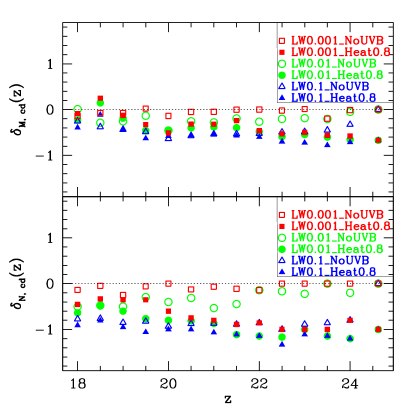
Figure 16.— This figure shows the suppression of cold dense gas in halos in simulations runs that include a persistent LW background. The LW background had specific intensities of $J_{\rm LW}=0.001,0.01$, or $0.1$ (normalized at 12.87 eV, in units of $10^{-21}{\rm ergs~{}s^{-1}~{}cm^{-2}~{}Hz^{-1}~{}sr^{-1}}$). Each of these three LW backgrounds is applied to both our NoUVB and Heat0.8 runs at $z=24.62$, and is subsequently left on. Values of $\delta_{M,{\rm cd}}(z)$ (top panel) and $\delta_{N,{\rm cd}}(z)$ (bottom panel) are show, as defined in equations (7) and (6).

5. Conclusions

We used three-dimensional hydrodynamic simulations to investigate the effects of a transient ultraviolet (UV) flux on the collapse and cooling of pregalactic clouds, with masses in the range $10^{5}$ – $10^{7}~{}M_{\odot}$, at high redshifts ($z\mathrel{\hbox to0.0pt{\lower 4.0pt\hbox{\hskip 1.0pt$\sim$}\hss}\raise 1.0pt\hbox{$>$}}18$). Although in the scenario we envision, the radiation is due to nearby PopIII star formation, in order to study its effect in a statistical way, we adopted a spatially constant but short-lived photo-ionizing background throughout the simulation box. This was done to mimic the effect of a $\sim 100$ solar mass star forming at $z=25$ and shining for 3 Myr. Of course, in reality, the closest star can be located at a range of distances and so we effectively covered this range by varying the strength of the background. The effect of the ionizing background will be strongest on relatively low density gas which is in the process of assembling to form halos at later times. The sign of the effect has been uncertain with suggestions of positive feedback due to enhanced H₂ formation, and negative feedback due to the increased entropy of gas in the relic HII region. In addition, we studied the combined effects of this transient UV flux and a persistent Lyman–Werner (LW) background (at photon energies below 13.6eV) from distant sources.

In the absence of a LW background, we find that a critical specific intensity of $J_{\rm UV}\sim 0.1\times 10^{-21}{\rm ergs~{}s^{-1}~{}cm^{-2}~{}Hz^{-1}~{}sr^{-1}}$ demarcates the transition from net negative to positive feedback for the halo population. A weaker UV flux stimulates subsequent star formation inside the fossil HII regions, by enhancing the ${\rm H_{2}}$ molecule abundance. A stronger UV flux significantly delays star–formation by reducing the gas density, and increasing the cooling time at the centers of collapsing halos. At a fixed $J_{\rm UV}$, the sign of the feedback also depends strongly on the density of the gas at the time of UV illumination. In either case, we find that once the UV flux is turned off, its impact starts to diminish after $\sim 30\%$ of the Hubble time.

In the more realistic case when a LW background is present (in addition to the ionizing source), with $J_{\rm LW}\mathrel{\hbox to0.0pt{\lower 4.0pt\hbox{\hskip 1.0pt$\sim$}\hss}\raise 1.0pt\hbox{$>$}}0.01\times 10^{-21}{\rm ergs~{}s^{-1}~{}cm^{-2}~{}Hz^{-1}~{}sr^{-1}}$, strong suppression persists down to the lowest redshift ($z=18$) in our simulations. Finally, we find evidence that heating and photoevaporation by the transient UV flux renders the $\sim 10^{6}~{}{\rm M_{\odot}}$ halos inside fossil HII regions more vulnerable to subsequent ${\rm H_{2}}$ photo–dissociation by a LW background.

The results of this study show that the combined negative feedback of a transient UV and a persistent LW background is effective at high redshift in suppressing star–formation in the low–mass halos; this suppression will help in delaying the reionization epoch to $z=6-10$ as inferred from SDSS quasar spectra and from CMB polarization anisotropy measurements in the 3–yr WMAP data.

Appendix A Comparing Semi-Analytic and Simulation Mass Functions

Although it is not directly relevant to the radiative feedback processes analyzed in the body of this paper, it is interesting to examine the mass function of dark matter halos we find in our simulations, and compare these to semi-analytic models. Such a comparison is especially interesting, since our simulation corresponds to a biased region that is overdense on the scale of the simulation box (rather than fixed to the cosmic mean density). We are not aware of a previous study of the halo mass function derived in such a biased region. Here we present a preliminary comparison, and postpone more detailed work for a future paper.

According to extended Press-Schechter formalism (EPS), the contribution of halos with masses greater than $M_{\rm min}$ to the mass fraction inside regions of mass scale $M$$\equiv$(4/3)$\pi$$R^{3}$$\langle\rho_{0}\rangle$ and extrapolated mean overdensity $\delta_{0}$, can be expressed as (e.g., Bond et al. 1991; Lacey & Cole 1993):

$$F_{\rm col}(>M_{\rm min},z)={\rm erfc}\left\{\frac{\delta_{c}(z)-\delta_{0}}{\sqrt{2[S(M_{\rm min})-S(M_{0})]}}\right\},$$ (A1)

where $\delta_{c}(z)$ is the critical linear overdensity at halo virialization, and $S(M)$ is the variance of the present-day linear overdensity field filtered on scale $M$. For comparison purposes below, we chose $M_{\rm min}=10^{5}M_{\odot}$.

To compare our numerical results with equation (A1), we chose our biasing scale, $M_{0}$, such that the enclosed spherical volume is equal to the volume of the refined region in the simulation, (4/3)$\pi$$R_{0}^{3}$ = $l_{\rm refined}^{3}$ = 1/64 $(h^{-1}~{}\rm Mpc)^{3}$, or equivalently, a mass scale of $M_{0}$ = $6.4\times 10^{8}~{}M_{\odot}$. Keeping in the spirit of the linear, Lagrangian nature of EPS, we obtain our overdensity bias, $\delta_{0}$, from the initial redshift of our simulation, $z_{\rm init}=99$, before the refined region in our Eulerian code has a chance to become too contaminated by inflow from outside particles. We obtain $\delta(z_{\rm init})=0.1637$ in our refined region, making our linear overdensity bias $\delta_{0}=\delta(z_{\rm init})/D(z_{\rm init})=12.8$.

We show the comparison of this biased mass fraction with our simulation in Figure 17. The solid line is determined by equation (A1), using the values quoted above. The points denote the values obtained from the cosmological simulation by summing over halos found with the HOP algorithm, in the case of no background radiation field. The dashed line is obtained by equation (A1), but for a mean sample of the universe (i.e. $\delta_{0}=0$, $S(M_{0})=0$).

                                                                                                                                                        

Figure 17.— Fraction of mass of the biased refined volume contained in halos with masses greater than $10^{5}M_{\odot}$. The solid line is determined from the extended Press–Schechter formalism, using equation (A1). The points denote the values obtained from the cosmological simulation by summing over halos found with the HOP algorithm, in the case of no background radiation field. The dashed line is obtained by equation (A1), but for a mean sample of the universe (i.e. $\delta_{0}=0$, $S(M_{0})=0$).

We note that mass fractions obtained from the simulation are a factor of $\sim 2$ lower than those obtained by EPS. To further probe this discrepancy, in Figure 18 we plot the analogous mass functions at $z=25$ (top panel) and $z=20$ (bottom panel). It is evident from the figure that abundance of low–mass halos is over-predicted by EPS with respect to the simulation, while the abundance of the largest halos in the simulation fits the EPS prediction fairly well.

This discrepancy might be due to several reasons. Firstly, it is already known that EPS mass-functions in the low–redshift regime suffer from similar over-predictions of low-mass halos, as well as an under-prediction of high-mass halos, where “low” and “high” are defined with respect to the characteristic collapse scale at $z$ (Jenkins et al., 2001; Sheth & Tormen, 1999), with the mass functions differing by up to a factor of $\sim 1.6$. Another contributing factor to the discrepancy could be the fact that the refined region of our simulation is a cubical perturbation, while parameters in the standard EPS are derived assuming spherical perturbations of the real-space density field. Finally, it has been shown that high–resolution cosmological simulations are too small to provide accurate mass functions at high redshifts, since they artificially cut-off the density modes larger than their box sizes (Barkana & Loeb, 2004). In particular, Barkana & Loeb (2004) show that at $z=20$, the true cosmic mean mass function can be a factor of several higher than would be derived from a (1 Mpc)³ simulation box, with periodic boundary conditions normalized to the mean density. Assuming that our biased simulation box suffers from a similar underestimate, the mass function could be consistent with the EPS prediction (after applying the correction proposed by Sheth & Tormen 1999).

Yoshida et al. (2003) have obtained a good fit at high redshifts ($z\sim 20$) between EPS mass functions and those obtained from simulations. Barkana & Loeb (2004) show that after correcting for the above missing large–scale power, that their results are consistent with the EPS mass function with the Sheth–Tormen correction. However, these results describe an unbiased simulation at mean density. We present the first comparison of the biased EPS and numerical mass functions at high redshifts. A detailed study on such a comparison is beyond the scope of this paper, nor does it have an impact on our main results.

                                                                                                                                                        

Figure 18.— Mass functions for the models analogous to Figure 17 at $z=25$ (top panel), and $z=20$ (bottom panel).

References

- Abel et al. (2002) Abel, T., Bryan, G. L., & Norman, M. L. 2002, Science, 295, 93
- Alvarez et al. (2006) Alvarez, M. A., Bromm, V., & Shapiro, P. R. 2006, ApJ, 639, 621
- Anninos & Norman (1996) Anninos, P., & Norman, M. L. 1996, ApJ, 460, 556
- Anninos et al. (1997) Anninos, P., Zhang, Y., Abel, T., & Norman, M. L. 1997, New Astronomy, 2, 209
- Barkana & Loeb (1999) Barkana, R., & Loeb, A. 1999, ApJ, 523, 54
- Barkana & Loeb (2004) —. 2004, ApJ, 609, 474
- Bond et al. (1991) Bond, J. R., Cole, S., Efstathiou, G., & Kaiser, N. 1991, ApJ, 379, 440
- Bromm et al. (2002) Bromm, V., Coppi, P. S., & Larson, R. B. 2002, ApJ, 564, 23
- Bromm & Loeb (2003) Bromm, V., & Loeb, A. 2003, Nature, 425, 812
- Bryan (1999) Bryan, G. L. 1999, Comput. Sci. Eng., 46, 1
- Cen (2003) Cen, R. 2003, ApJ, 591, L5
- Ciardi et al. (2000) Ciardi, B., Ferrara, A., & Abel, T. 2000, ApJ, 533, 594
- Efstathiou (1992) Efstathiou, G. 1992, MNRAS, 256, 43P
- Eisenstein & Hu (1999) Eisenstein, D. J., & Hu, W. 1999, ApJ, 511, 5
- Eisenstein & Hut (1998) Eisenstein, D. J., & Hut, P. 1998, ApJ, 498, 137
- Fan et al. (2006) Fan, X., Carilli, C. L., & Keating, B. 2006, ARA&A, in press, preprint astro-ph/0602375
- Galli & Palla (1998) Galli, D., & Palla, F. 1998, A&A, 335, 403
- Gnedin & Abel (2001) Gnedin, N. Y., & Abel, T. 2001, New Astronomy, 6, 437
- Haiman et al. (2001) Haiman, Z., Abel, T., & Madau, P. 2001, ApJ, 551, 599
- Haiman et al. (2000) Haiman, Z., Abel, T., & Rees, M. J. 2000, ApJ, 534, 11
- Haiman & Bryan (2006) Haiman, Z., & Bryan, G. L. 2006, ApJL, submitted, preprint astro-ph/0603541
- Haiman & Holder (2003) Haiman, Z., & Holder, G. P. 2003, ApJ, 595, 1
- Haiman et al. (1996) Haiman, Z., Rees, M. J., & Loeb, A. 1996, ApJ, 467, 522
- Haiman et al. (1997) —. 1997, ApJ, 484, 985
- Iliev et al. (2006) Iliev, I. T. et al. 2006, MNRAS, submitted, preprint astro-ph/0603199
- Iliev et al. (2005) Iliev, I. T., Shapiro, P. R., & Raga, A. C. 2005, MNRAS, 361, 405
- Jenkins et al. (2001) Jenkins, A., Frenk, C. S., White, S. D. M., Colberg, J. M., Cole, S., Evrard, A. E., Couchman, H. M. P., & Yoshida, N. 2001, MNRAS, 321, 372
- Kitayama et al. (2004) Kitayama, T., Yoshida, N., Susa, H., & Umemura, M. 2004, ApJ, 613, 631
- Kuhlen & Madau (2005) Kuhlen, M., & Madau, P. 2005, MNRAS, 363, 1069
- Lacey & Cole (1993) Lacey, C., & Cole, S. 1993, MNRAS, 262, 627
- Liddle et al. (1996) Liddle, A. R., Lyth, D. H., Viana, P. T. P., & White, M. 1996, MNRAS, 282, 281
- Machacek et al. (2001) Machacek, M. E., Bryan, G. L., & Abel, T. 2001, ApJ, 548, 509
- Machacek et al. (2003) —. 2003, MNRAS, 338, 273
- MacIntyre et al. (2005) MacIntyre, M. A., Santoro, F., & Thomas, P. A. 2005, astro-ph/0510074
- Mesinger & Haiman (2004) Mesinger, A., & Haiman, Z. 2004, ApJ, 611, L69
- Norman & Bryan (1999) Norman, M. L., & Bryan, G. L. 1999, in ASSL Vol. 240: Numerical Astrophysics, 19–+
- Oh & Haiman (2002) Oh, S. P., & Haiman, Z. 2002, ApJ, 569, 558
- Oh & Haiman (2003) —. 2003, MNRAS, 346, 456
- Omukai (2000) Omukai, K. 2000, ApJ, 534, 809
- O’Shea et al. (2005) O’Shea, B. W., Abel, T., Whalen, D., & Norman, M. L. 2005, ApJ, 628, L5
- Page et al. (2006) Page, L. et al. 2006, ApJ, submitted
- Ricotti et al. (2002a) Ricotti, M., Gnedin, N. Y., & Shull, J. M. 2002a, ApJ, 575, 33
- Ricotti et al. (2002b) —. 2002b, ApJ, 575, 49
- Scannapieco et al. (2002) Scannapieco, E., Ferrara, A., & Madau, P. 2002, ApJ, 574, 590
- Scannapieco et al. (2003) Scannapieco, E., Schneider, R., & Ferrara, A. 2003, ApJ, 589, 35
- Schaerer (2002) Schaerer, D. 2002, A&A, 382, 28
- Shapiro et al. (2004) Shapiro, P. R., Iliev, I. T., & Raga, A. C. 2004, MNRAS, 348, 753
- Shapiro & Kang (1987) Shapiro, P. R., & Kang, H. 1987, ApJ, 318, 32
- Sheth & Tormen (1999) Sheth, R. K., & Tormen, G. 1999, MNRAS, 308, 119
- Spergel et al. (2006a) Spergel, D. N. et al. 2006a, ApJ, submitted, preprint astro-ph/0603449
- Spergel et al. (2006b) —. 2006b, ApJ, submitted
- Spergel et al. (2003) —. 2003, ApJS, 148, 175
- Susa et al. (1998) Susa, H., Uehara, H., Nishi, R., & Yamada, M. 1998, Progress of Theoretical Physics, 100, 63
- Whalen et al. (2004) Whalen, D., Abel, T., & Norman, M. L. 2004, ApJ, 610, 14
- Wyithe & Loeb (2003) Wyithe, J. S. B., & Loeb, A. 2003, ApJ, 588, L69
- Yoshida et al. (2003) Yoshida, N., Sokasian, A., Hernquist, L., & Springel, V. 2003, ApJ, 591, L1