Low $T/|W|$ dynamical instabilities in differentially rotating stars: Diagnosis with canonical angular momentum

Abstract

We study the nature of non-axisymmetric dynamical instabilities in differentially rotating stars with both linear eigenmode analysis and hydrodynamic simulations in Newtonian gravity. We especially investigate the following three types of instability; the one-armed spiral instability, the low $T/|W|$ bar instability, and the high $T/|W|$ bar instability, where $T$ is the rotational kinetic energy and $W$ is the gravitational potential energy. The nature of the dynamical instabilities is clarified by using a canonical angular momentum as a diagnostic. We find that the one-armed spiral and the low $T/|W|$ bar instabilities occur around the corotation radius, and they grow through the inflow of canonical angular momentum around the corotation radius. The result is a clear contrast to that of a classical dynamical bar instability in high $T/|W|$. We also discuss the feature of gravitational waves generated from these three types of instability.

1 Introduction

Stars in nature are usually rotating and may be subject to non-axisymmetric rotational instabilities. An analytically exact treatment of these instabilities in linearized theory exists only for incompressible equilibrium fluids in Newtonian gravity (e.g., Chandrasekhar, 1969). For these configurations, global rotational instabilities may arise from non-radial toroidal modes $e^{im\varphi}$ (where $m=\pm 1,\pm 2,\dots$ and $\varphi$ is the azimuthal angle).

For sufficiently rapid rotation, the $m=2$ bar mode becomes either secularly or dynamically unstable. The onset of instability can typically be marked by a critical value of the dimensionless parameter $\beta\equiv T/|W|$, where $T$ is the rotational kinetic energy and $W$ the gravitational potential energy. Uniformly rotating, incompressible stars in Newtonian theory are secularly unstable to bar-mode formation when $\beta\gtrsim\beta_{\rm sec}\simeq 0.14$. This instability can grow only in the presence of some dissipative mechanism, like viscosity or gravitational radiation, and the associated growth time-scale is the dissipative time-scale, which is usually much longer than the dynamical time-scale of the system. By contrast, a dynamical instability to bar formation sets in when $\beta\gtrsim\beta_{\rm dyn}\simeq 0.27$. This instability is present independent of any dissipative mechanism, and the growth time is the hydrodynamic time-scale.

In addition to the classical dynamical instability mentioned above, there have been several studies indicating that a dynamical instability of the rotating stars occurs at low $T/|W|$, which is far below the classical criterion of dynamical instability in Newtonian gravity. Tohline and Hachisu (1990) find in the self-gravitating ring and tori that an $m=2$ dynamical instability occurs around $T/|W|\sim 0.16$ in the lowest case in the centrally condensed configurations. For rotating stellar models, Shibata, Karino and Eriguchi (2002;2003) find that $m=2$ dynamical instability occurs around $T/|W|\sim O(10^{-2})$ for a high degree ($\Omega_{\rm c}/\Omega_{\rm s}\approx 10$) of differential rotation. Note that $\Omega_{\rm c}$ and $\Omega_{\rm s}$ are the angular velocity at the centre and at the equatorial surface, respectively. Centrella et al. (2001) found dynamical $m=1$ instability around $T/|W|\sim 0.09$ in the $N=3.33$ polytropic “toroidal” star with a high degree ($\Omega_{\rm c}/\Omega_{\rm s}=26$) of differential rotation, and Saijo, Baumgarte and Shapiro (2003) extended the results of dynamical $m=1$ instability to the cases with polytropic index $N\gtrsim 2.5$ and $\Omega_{\rm c}/\Omega_{\rm s}\gtrsim 10$.

Computation of the onset of the dynamical instability, as well as the subsequent evolution of an unstable star, performed in a fully nonlinear hydrodynamic simulation in Newtonian gravity have shown that $\beta_{\rm dyn}$ depends only very weakly on the stiffness of the equation of state. Once a bar has developed, the formation of a two-arm spiral plays an important role in redistributing the angular momentum and forming a core-halo structure. $\beta_{\rm dyn}$ are smaller for stars with high degree of differential rotation (Tohline and Hachisu, 1990; Shibata et al., 2002;2003; Pickett, Durisen and Davis, 1996). Simulations in relativistic gravitation (Shibata et al., 2000; Saijo et al., 2001) have shown that $\beta_{\rm dyn}$ decreases with the compaction of the star, indicating that relativistic gravitation enhances the bar mode instability.

One of the remarkable features of these low $T/|W|$ instabilities is an appearance of the corotation modes. As it is pointed out by Watts, Andersson and Jones (2005) the low $T/|W|$ unstable oscillation of bar-typed one found by Shibata et al. (2002;2003) has a corotation point. Here corotation means the pattern speed of oscillation in the azimuthal direction coincides with a local rotational angular velocity of the star. It is well-known in the context of stellar or gaseous disk system that the corotation of oscillation may lead to instabilities. For instance, there have been several density wave models proposed to explain spiral pattern in galaxies, in which wave amplification at the corotation radius of spiral pattern is a key issue. Another example of importance of corotation is found in the theory of thick disk (torus) around black holes. Initiated by a discovery of a dynamical instability of geometrically thick disk by Papaloizou and Pringle (1984). Instabilities of these systems are thought not to be unique in their origin and in their characteristics. Some seem to be related to local shear of flow and to share a nature with Kelvin-Helmholtz instability. Others may be related to corotation of oscillation modes with averaged flow on which the oscillation is present. The mechanisms of instabilities by corotation, however, seem not unique. As is reminiscent to “Landau amplification” of plasma wave, a resonant interaction of corotating wave with the background flow (in the case of Landau amplification, background flow is that of charged particles) may amplify the wave, by direct pumping of energy from background flow to the oscillation. The other may be an overreflection of waves at the corotation which may be seen in waves propagating towards shear layer.

The main purpose of this paper, in contrast to the preceding studies of this issue, is to investigate the nature of low $T/|W|$ dynamical instabilities, especially to study the qualitative difference of them from the classical bar instability. As is mentioned above, recent studies have shown that dynamical instabilities are possible for different region of the parameter space of rotating stars. Observing the existence of dynamical instabilities whose critical $T/|W|$ value are well below the classical criterion of bar instability, it is natural to raise a question on whether these two types, “high $T/|W|$” and “low $T/|W|$”, of dynamical instability are categorized in the same type of dynamical instability or not.

Our study is done with both eigenmode analysis and hydrodynamical analysis. A non-linear hydrodynamical simulation is indispensable for investigation of evolutionary process and final outcome of instability, such as bar formation and spiral structure formation. The nature of instability as a source of gravitational wave, which interests us most, is only accessible through non-linear hydrodynamical computations. On the other hand, a linear eigenmode analysis is in general easier to approach the dynamical instability of a given equilibrium and it may be helpful to have physical insight on the mechanism and the origin of the instability. Therefore, a linear eigenmode analysis and a non-linear simulation are complementary to each other and they both help us to understand the nature of dynamical instability.

As a simplified system mimicking the physical nature of the differentially rotating fluid, we choose to study self-gravitating cylinder models. They have been used to study general dynamical nature of such gaseous masses as stars, accretion disks and of stellar system as galaxies. Although there is no infinite-length cylinder in the real world, it is expected to share some qualitative similarities with realistic astrophysical objects (e.g. Ostriker, 1965). Especially it has served as a useful model to investigate secular and dynamical instabilities of rotating masses. These works took advantage of a simple configuration of a cylinder compared with a spheroid.

This paper is organized as follows. In the section: Dynamical instabilities in differentially rotating stars, we present our hydrodynamical results of dynamical one-armed spiral and dynamical bar instabilities. We present our diagnosis of dynamical $m=1$ and $m=2$ instabilities by using a canonical angular momentum in the section: Canonical angular momentum to diagnose dynamical instability, and summarize our findings in the section: Summary and discussion. Throughout this paper we use gravitational units with $G=1$. Latin indices run over spatial coordinates. A more detailed discussion is presented in Saijo and Yoshida (2006).

2 Dynamical Instabilities in Differentially Rotating Stars

We explain three types of dynamical instabilities in differentially rotating stars based on non-linear hydrodynamical computations. We assume a polytropic equation of state only to construct an equilibrium star as

$$P=\kappa\rho^{1+1/N},$$ (1)

where $P$ is a pressure, $\rho$ a rest-mass density, $\kappa$ a constant, $N$ the polytropic index. We also assume the “$j$-constant” rotation law, which has an exact meaning in the limit of $d\rightarrow 0$, of the rotating stars

$$\Omega=\frac{j_{0}}{d^{2}+\varpi^{2}},$$ (2)

where $\Omega$ is the angular velocity, $j_{0}$ a constant parameter with units of specific angular momentum, and $\varpi$ the cylindrical radius. The parameter $d$ determines the length scale over which $\Omega$ changes; uniform rotation is achieved in the limit $d\rightarrow\infty$, with keeping the ratio $j_{0}/d^{2}$ finite. We choose the same data sets as Saijo et al. (2003) for investigating low $T/|W|$ dynamical instabilities in differentially rotating stars (models I and II in Table 1 corresponds to Tables II and I of Saijo et al. (2003), respectively). We also construct an equilibrium star with weak differential rotation in high $T/|W|$, which excites the standard dynamical bar instability, (e.g., Chandrasekhar, 1969). The characteristic parameters are summarized in Table 1.

Model	$N$	$d/R_{\rm eq}$	$R_{\rm pl}/R_{\rm eq}$	$\Omega_{\rm c}/\Omega_{\rm s}$	$\rho_{\rm c}/\rho_{\rm max}$	$R_{\rm maxd}/R_{\rm eq}$	$T/|W|$	Dominant unstable mode
I	$3.33$	$0.20$	$0.413$	$26.0$	$0.491$	$0.198$	$0.146$	$m=1$
II	$1.00$	$0.20$	$0.250$	$26.0$	$0.160$	$0.383$	$0.119$	$m=2$
III	$1.00$	$1.00$	$0.250$	$2.0$	$0.837$	$0.388$	$0.277$	$m=2$

Table 1: Three differentially rotating equilibrium stars that trigger dynamical instability

To enhance any $m=1$ or $m=2$ instability, we disturb the initial equilibrium mass density $\rho_{\rm eq}$ by a non-axisymmetric perturbation according to

$$\rho=\rho_{\rm eq}\left(1+\delta^{(1)}\frac{x+y}{R_{\rm eq}}+\delta^{(2)}\frac{x^{2}-y^{2}}{R_{\rm eq}^{2}}\right),$$ (3)

where $R_{\rm eq}$ is the equatorial radius, with $\delta^{(1)}=\delta^{(2)}\approx 1.7-2.8\times 10^{-3}$ in all our simulations. We also introduce “dipole” $D$ and “quadrupole” $Q$ diagnostics to monitor the development of $m=1$ and $m=2$ modes as

$$D = \left<e^{im\varphi}\right>_{m=1}=\frac{1}{M}\int\rho\frac{x+iy}{\varpi}dV,$$ (4)

$$Q = \left<e^{im\varphi}\right>_{m=2}=\frac{1}{M}\int\rho\frac{(x^{2}-y^{2})+i(2xy)}{\varpi^{2}}dV,$$ (5)

respectively.

We compute approximate gravitational waveforms by using the quadrupole formula. In the radiation zone, gravitational waves can be described by a transverse-traceless, perturbed metric $h_{ij}^{TT}$ with respect to flat spacetime. In the quadrupole formula, $h_{ij}^{TT}$ is found from

$$h_{ij}^{TT}=\frac{2}{r}\frac{d^{2}}{dt^{2}}I_{ij}^{TT},$$ (6)

where $r$ is the distance to the source, $I_{ij}$ the quadrupole moment of the mass distribution, and where $TT$ denotes the transverse-traceless projection. Choosing the direction of the wave propagation to be along the rotational axis ($z$-axis), the two polarization modes of gravitational waves can be determined from

$$h_{+}\equiv\frac{1}{2}(h_{xx}^{TT}-h_{yy}^{TT}),\quad h_{\times}\equiv h_{xy}^{TT}.$$ (7)

For observers along the rotation axis, we thus have

$$\frac{rh_{+}}{M} = \frac{1}{2M}\frac{d^{2}}{dt^{2}}(I_{xx}^{TT}-I_{yy}^{TT}),$$ (8)

$$\frac{rh_{\times}}{M} = \frac{1}{M}\frac{d^{2}}{dt^{2}}I_{xy}^{TT}.$$ (9)

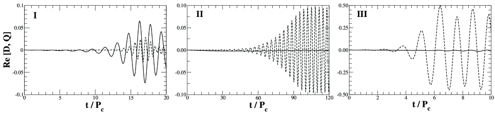
Figure 1: Diagnostics $D$ and $Q$ as a function of $t/P_{\rm c}$ for three differentially rotating stars (see Table 1). Solid and dotted lines denote the values of $D$ and $Q$, respectively. The Roman numeral in each panel corresponds to the model of the differentially rotating stars, respectively. Hereafter $P_{\rm c}$ represents the central rotation period at $t=0$.

The time evolutions of the dipole diagnostic and the quadrupole diagnostic are plotted in Figure 1. We determine that the system is stable to $m=1$ ($m=2$) mode when the dipole (quadrupole) diagnostic remains small throughout the evolution, while the system is unstable when the diagnostic grows exponentially at the early stage of the evolution. It is clearly seen in Figure 1 that the star is more unstable to the one-armed spiral mode for model I, and more unstable to the bar mode for models II and III. In fact, both diagnostics grow for model I. The dipole diagnostic, however, grows larger than the quadrupole diagnostic, indicating that the $m=1$ mode is the dominant unstable mode.

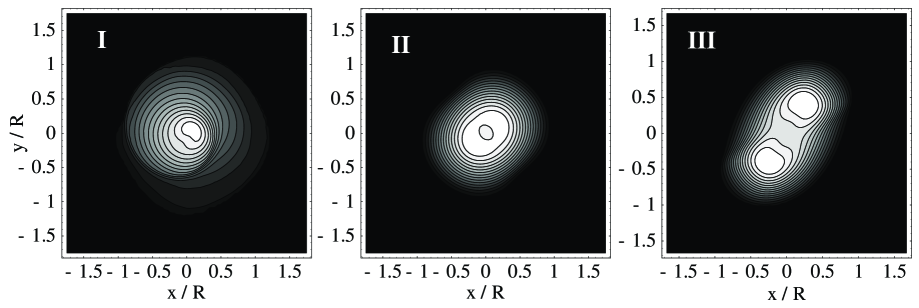
Figure 2: Density contours in the equatorial plane for three differentially rotating stars (see Table 1). Models I, II, and III are plotted at the parameter ($t/P_{\rm c}$, $\rho_{\rm max}/\rho_{\rm max}^{(0)}$) = ($16.2$, $3.63$), ($134$, $1.26$), and ($5.49$, $1.20$), where $\rho_{\rm max}$ is the maximum density, $\rho_{\rm max}^{(0)}$ is the maximum density at $t=0$, and $R$ is the equatorial radius at $t=0$. The contour lines denote densities $\rho/\rho_{\rm max}=10^{-(16-i)\times 0.287}(i=1,\cdots,15)$ for model I and $\rho/\rho_{\rm max}=6.67(16-i)\times 10^{-2}(i=1,\cdots,15)$ for models II and III, respectively.

The density contour of the differentially rotating stars are shown in Figure 2 for the equatorial plane. It is clearly seen in Figure 2 that one-armed spiral structure is formed at the intermediate stage of the evolution for model I, and that bar structure is formed for models II and III once the dynamical instability sets in.

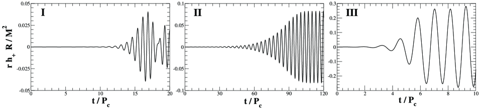
Figure 3: Gravitational waveform for three differentially rotating stars (see Table 1) as seen by a distant observer located on the rotational axis of the equilibrium star.

We also show gravitational waves generated from dynamical one-armed spiral and bar instabilities in Figure 3. For $m=1$ modes, the gravitational radiation is emitted not by the primary mode itself, but by the $m=2$ secondary harmonic which is simultaneously excited, albeit at the lower amplitude. Unlike the case for bar-unstable stars, the gravitational wave signal does not persist for many periods, but instead damp fairly rapidly.

Model	$\Omega_{\rm c}/\Omega_{\rm s}$	$T/|W|$	$\sigma/\Omega_{\rm c}$	$\varpi_{\rm{crt}}/\varpi_{\rm s}$
A-i	11.34	0.460	$-0.245$	—
A-ii	11.34	0.460	$0.551+0.0315i$	0.281
A-iii	11.34	0.460	$1.15$	—
B	13.00	0.170	$0.327+0.0126i$	0.507

Table 2: Parameters for equilibrium gaseous fluid and eigenfrequency

3 Canonical Angular Momentum to Diagnose Dynamical Instability

We introduce the canonical angular momentum following Friedman and Schutz (1978) to diagnose the oscillations in rotating fluid. In the theory of adiabatic linear perturbations of a perfect fluid configuration with some symmetries, it is possible to introduce canonical conserved quantities associated with the symmetries. Since we only use canonical angular momentum $J_{\rm c}$ in this paper, we write down its explicit form as

$$J_{\rm c}=m\int_{V}(\Re[\sigma]-m\Omega)\rho|\xi|^{2}dV-2m\int_{V}\rho\varpi\Omega\cdot\Im[\xi^{\varpi}\xi^{\varphi*}]dV,$$ (10)

where $\sigma$ is the eigenfrequency, $\xi^{i}$ is Lagrangian displacement vector. Note that total canonical angular momentum becomes zero when dynamical instability sets in.

Next we apply the method of canonical angular momentum to the linearized oscillations of a cylinder. We prepare two $m=1$ stable modes (A-i, A-iii) and one $m=1$ unstable mode (A-ii), summarized in Table 2. We plot the integrand of canonical angular momentum $\varpi j_{\rm c}$

$$\varpi j_{\rm c}(\varpi)=m(\Re[\sigma]-m\Omega)\rho|\xi|^{2}-2m\rho\varpi\Omega\cdot\Im[\xi^{\varpi}\xi^{\varphi*}],$$ (11)

for $m=1$ mode in Figure 6. We define corotation radius $\varpi_{\rm crt}$ of modes as $\Re[\sigma]-m\Omega(\varpi)=0$. This means that the pattern speed of mode coincides with the local rotational frequency of background flow there. Note that an integral in the entire cylinder is zero for these cases. The features of the canonical angular momentum distribution for $m=1$ unstable modes are,

1. It changes sign around corotation radius $\varpi_{\rm crt}$.

2. It is positive for $\varpi<\varpi_{\rm crt}$, while negative for $\varpi>\varpi_{\rm crt}$.

The feature 1 is remarkable and suggests us that the instability is related to the corotation. The feature has a clear contrast for a stable mode (Figure 4). The canonical angular momentum is either positive or negative definite, and it does not change its sign. Note that the former is the case when the pattern speed of mode is faster than the rotation of cylinder everywhere, while the latter is the opposite. This feature is expected from the equation (10), if the first term is dominant. In such case, the sign of $\Re[\sigma]-m\Omega(\varpi)$ determines the sign of the canonical angular momentum. This simple interpretation, however, does not hold for the dynamically unstable mode. As it is shown in the feature 2 above, we have a positive canonical angular momentum inside the corotation, which is opposite to the sign of $\sigma-\Omega(\varpi)$ for $0\leq\varpi<\varpi_{\rm crt}$.

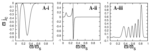
Figure 4: Distribution of canonical angular momentum density for $m=1$ unstable mode (see Table 2). Vertical dashed line represents the location of corotation radius of the mode. The Roman character in each panel corresponds to the model of the cylindrical gaseous fluid, respectively. Note that we normalized the distribution of the canonical angular momentum in an appropriate value, since the eigenfunction can be scaled arbitrarily.

In Figure 5, we show an example of canonical angular momentum distribution for $m=2$ unstable mode of differentially rotating cylinder, which may be compared with the low $T/|W|$ bar instability of Shibata et al. (2002;2003). We did not find $m=2$ unstable modes for the same parameters as in the case of $m=1$ instability. The features at the corotation radius, however, are the same as in $m=1$ instability.

It is interesting to see how the profile of the canonical angular momentum changes when we consider the classical bar instability with uniform rotation. Unfortunately the bar mode of uniformly rotating cylinder has a neutral stability point at the breakup limit. We instead looked at $m=2$ instability of uniformly rotating, incompressible Bardeen disk (Bardeen, 1975) and the classical bar instability of Maclaurin spheroid. These are actually more suitable for comparison to differentially rotating spheroidal model, which we present in the following section. For both of the models we have analytic expressions of oscillation modes. It is remarkable that the canonical angular momentum density is zero everywhere (which ensures that the total canonical angular momentum vanishes). This is in a clear contrast with the $m=2$ instability in the cylinder with highly differential rotation.

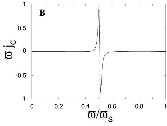
Figure 5: Distribution of canonical angular momentum density for $m=2$ unstable mode (see Table 2). The Roman character in the panel corresponds to the model of the cylindrical gaseous fluid. Vertical dashed lines mark the locations of corotation radius of the mode.

Model	$\sigma$ $[\Omega_{\rm c}]$	$\varpi_{\rm crt}$ $[R_{\rm eq}]$
I	$0.590+0.0896i$	$0.167$
II	$0.284+0.0121i$	$0.492$
III	$0.757+0.200i$	—

Table 3: Eigenfrequency and the corotation radius of three differentially rotating stars

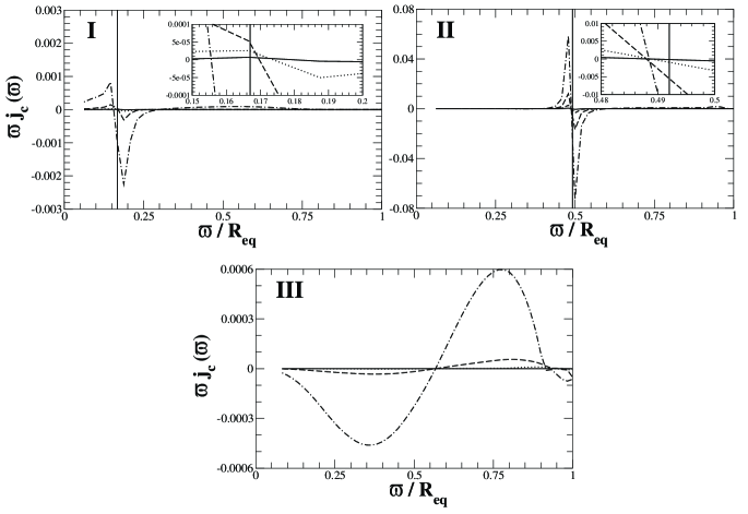
Figure 6: Snapshots of the canonical angular momentum distribution $\varpi j_{\rm c}(\varpi)$ in the equatorial plane for three differentially rotating stars (see Table 1). Solid, dotted, dashed, and dash-dotted line represents the time $t/P_{\rm c}=$(3.47, 6.93, 10.40, 13.86) for model I, $t/P_{\rm c}=$(45.68, 56.43, 67.18, 77.97) for model II, and $t/P_{\rm c}=$(1.10, 2.19, 3.29, 4.39) for model III, respectively. Note that vertical line in panels I and II denotes the corotation radius of the star (model III does not have a corotation radius). We also enlarged the figure around the corotation radius for panels I and II, which is presented in the right upper part of each panel. Although our method of determining the corotation radius is not precise, we clearly find that the distribution significantly changes around the corotation radius.

Finally, we adopt the method of canonical angular momentum to the nonlinear hydrodynamics. We identify the complex eigenfrequency and the corotation radius from dipole or quadrupole diagnostics which is summarized in Table 3. Note that we read off the eigenfrequency from those plots at the early stage of the evolution. The Eulerian perturbed velocity is defined by subtracting the velocity at equilibrium from the velocity. The Lagrangian displacement vector is extracted by using a linear formula for a dominant mode in each case.

We show the snapshots of canonical angular momentum density in Figure 6. Since we determine the corotation radius using the extracted eigenfrequency and the angular velocity profile at equilibrium, the radius does not change throughout the evolution. For low $T/|W|$ dynamical instability, the distribution of the canonical angular momentum drastically changes its sign around the corotation radius, and the maximum amount of canonical angular momentum density increases at the early stage of evolution. This means that the angular momentum flows inside the corotation radius in the evolution. On the other hand, for high $T/|W|$ dynamical instability (Panel III of Figure 6), which may be regarded as a classical bar instability modified by differential rotation, the distribution of the canonical angular momentum is smooth and with no particular feature.

Note that the amplitude of $\varpi j_{c}$ is orders of magnitude smaller than those in the corotating cases in top and middle panels of Figure 6. Contrary to the linear perturbation analysis, the amplitude here is not scale free and the relative amplitude has a physical meaning. Thus the smallness of it for model III suggest that it should be exactly zero everywhere in the limit of linearized oscillation. The deviation from zero may come from the imperfect assumption of linearized oscillation, that is made here to extract oscillation frequency and Lagrangian displacement vector.

From these different behaviours of the distribution of the canonical angular momentum, we find that the mechanisms working in the low $T/|W|$ instabilities and the classical bar instability may be quite different, i.e., in the former the corotation resonance of modes are essential, while the instability is global in the latter case.

4 Summary and Discussion

We have studied the nature of three different types of dynamical instability in differentially rotating stars both in linear eigenmode analysis and in hydrodynamic simulation using canonical angular momentum distribution.

We have found that the low $T/|W|$ dynamical instability occurs around the corotation radius of the star by investigating the distribution of the canonical angular momentum. We have also found by investigating the canonical angular momentum that the instability grows through the inflow of the angular momentum inside the corotation radius. The feature also holds for the dynamical bar instability in low $T/|W|$, which is in clear contrast to that of classical dynamical bar instability in high $T/|W|$. Therefore the existence of corotation point inside the star plays a significant role of exciting one-armed spiral mode and bar mode dynamically in low $T/|W|$. However, we made our statement from the behaviour of the canonical angular momentum, the statement holds only in a sense of necessary condition. In order to understand the physical mechanism of the low $T/|W|$ dynamical instability, we need another tool and it will be the next step of this study.

The feature of gravitational waves generated from these instabilities are also compared. Quasi-periodic gravitational waves emitted by stars with $m=1$ instabilities have smaller amplitudes than those emitted by stars unstable to the $m=2$ bar mode. For $m=1$ modes, the gravitational radiation is emitted not directly by the primary mode itself, but by the $m=2$ secondary harmonic which is simultaneously excited. Possibly this $m=2$ oscillation is generated through a quadratic nonlinear selfcoupling of $m=1$ eigenmode. Remarkably the precedent studies (Centrella et al., 2001; Saijo et al., 2003) found that the pattern speed of $m=2$ mode is almost the same as that of $m=1$ mode, which suggest the former is the harmonic of the latter. Unlike the case for bar-unstable stars, the gravitational wave signal does not persist for many periods, but instead is damped fairly rapidly. We have not understood this remarkable difference between $m=1$ and $m=2$ unstable cases. One of the possibility may be that the unstable $m=1$ eigenmode tends to couple to higher and higher $m$ modes (which are not necessarily unstable and could be in the continuous spectrum) and pump its energy to them in a cascade way. However, we have not found the feature that prevents $m=2$ mode from this cascade dissipation.

Another possibility is that the spiral pattern formed in $m=1$ instability redistributes the angular momentum of the original unstable flow, so that the flow is quickly stabilized. Inside the corotation radius, the background flow is faster than the pattern, while it is slower outside. A similar mechanism to Landau damping in plasma wave which transfer the momentum of wave to background flow may work at the spiral pattern. The pattern may decelerate the background flow inside the corotation and accelerate it outside the corotation, which may change the unstable flow profile to stable one. As we do not see a spiral pattern forming in the low $T/|W|$ bar instability, it may eludes this damping process.

References

- Chandrasekhar (1969) S. Chandrasekhar, Ellipsoidal Figures of Equilibrium, Yale Univ. Press, New York, 1969, Chap. 5, Sec. 33.
- Tohline and Hachisu (1990) J. E. Tohline and I. Hachisu, Astrophys. J. 361, 394 (1990).
- Shibata et al. (2002;2003) M. Shibata, S. Karino and Y. Eriguchi, Mon. Not. R. Astron. Soc. 334, L27 (2002); 343, 629 (2003).
- Centrella et al. (2001) J. M. Centrella, K. C. B. New, L. L. Lowe and J. D. Brown, Astrophys. J. Lett. 550, L193 (2001).
- Saijo et al. (2003) M. Saijo, T. W. Baumgarte and S. L. Shapiro, Astrophys. J. 595, 352 (2003).
- Pickett, Durisen and Davis (1996) B. K. Pickett, R. H. Durisen and G. A. Davis, Astrophys. J. 458, 714 (1996).
- Shibata et al. (2000) M. Shibata, T. W. Baumgarte and S. L. Shapiro, Astrophys. J. 542, 453 (2000).
- Saijo et al. (2001) M. Saijo, M. Shibata, T. W. Baumgarte and S. L. Shapiro, Astrophys. J. 548, 919 (2001).
- Watts et al. (2005) A. L. Watts, N. Andersson and D. I. Jones, Astrophys. J. Lett. 618, L37 (2005).
- Papaloizou and Pringle (1984) J. C. B. Papaloizou and J. E. Pringle, Mon. Not. R. Astron. Soc. 208, 721 (1984).
- Ostriker (1965) J. Ostriker, Astrophys. J. Suppl. 11, 167 (1965).
- Saijo and Yoshida (2006) M. Saijo and S’i. Yoshida, Mon. Not. R. Astron. Soc. , in press (2006); astro-ph/0505543.
- Friedman and Schutz (1978) J. L. Friedman and B. F. Schutz, Astrophys. J. 221, 937 (1978).
- Bardeen (1975) J. M. Bardeen, in Dynamics of Stellar Systems; Proceedings of IAU Symposium 69, edited by A. Hayli, Reidel, Dordrecht, 1975, pp. 297 – 320.