Stellar populations in the nuclei of late-type spiral galaxies

Abstract

As part of an ongoing effort to study the stellar nuclei of very late-type, bulge-less spirals, we present results from a high-resolution spectroscopic survey of nine such nuclear star clusters, undertaken with VLT/UVES. We fit the spectra with population synthesis models and measure Lick-type indices to determine mean luminosity-weighted ages, which range from $4.1\times 10^{7}$ to $1.1\times 10^{10}$ years and are insensitive to assumed metallicity or internal extinction. The average metallicity of nuclear clusters in late-type spirals is slightly sub-solar ($\langle Z\rangle=0.015$) but shows significant scatter. Most of the clusters have moderate extinctions of 0.1 to 0.3 mags in the $I$-band. The fits also show that the nuclear cluster spectra are best described by a mix of several generations of stars. This is supported by the fact that only models with composite stellar populations yield mass-to-light ratios that match those obtained from dynamical measurements. For our nine sample clusters, the last star formation episode was on average 34 Myr ago, while all clusters experienced some star formation in the last 100 Myr. We thus conclude that the nuclear clusters undergo repeated episodes of star formation. The robustness of our results with respect to possible contamination from the underlying galaxy disk is demonstrated by comparison to a similar analysis using smaller-aperture spectra obtained with HST/STIS. Combining these results with those from Walcher et al. (2005), we have thus shown that the stellar nuclei of these bulge-less galaxies are massive and dense star clusters that form stars recurrently until the present day. This set of properties is unique among the various classes of star clusters. It is almost inevitable to associate these unique properties with the location of the cluster in its host galaxy. It remains a challenging question to elucidate exactly how very late-type spirals manage to create nuclei with such extreme characteristics.

1 Introduction

Galaxy centers have attracted special interest from astronomers for a long time, as they are the places of a number of distinctive phenomena, such as active galactic nuclei, central starbursts and extremely high stellar densities. The last decade has also shown that the evolution of galaxies is closely linked to the evolution of their nuclei, as evidenced by a number of global to nucleus relations (Ferrarese & Merrit 2000; Gebhardt et al. 2000; Graham et al. 2001; Ferrarese 2002; Häring & Rix 2004). In view of this general paradigm we here present our ongoing efforts to study the nuclear star clusters in late-type spirals as a contribution to a full census of galaxy nuclei over all Hubble types.

It has been thought for 20 years that “the centers of some, perhaps most, galaxies contain a nuclear stellar system which is dynamically distinct from the surrounding bulge or disk components” (O’Connell 1983). Indeed, in our close vicinity, nuclear star clusters (NCs) are found in the Galactic center (Krabbe et al. 1995; Genzel & Eckart 1998), in M31 (Johnson 1961; Davidge 1997; Lauer et al. 1998), and in M33 (Gallagher, Goad & Mould 1982). We here reserve the word NC for the one central star cluster of a galaxy, which is in the dynamic center of the galaxy, i.e. at the bottom of its potential well. On a larger scale, Phillips et al. (1996) and Matthews & Gallagher (1997) surveyed the nuclei of nearby spirals and found NCs in 6 out of 10 and in 10 out of 49 late-type spirals, respectively (see also Matthews et al. 1999). Subsequently, Carollo et al. (1997) and Carollo, Stiavelli & Mack (1998) found nuclear point-like sources to be present in many of the nearby spiral galaxies in their sample. Further down the Hubble sequence exist such examples as the bright, central cluster in NGC 1705 (Ho & Filippenko, 1996), a dwarf irregular galaxy. Also active galaxies are observed to host NCs in some cases (e.g., Thatte et al. 1997; Gallimore & Matthews 2003; Schinnerer et al. 2001). In the specific case of late-type spirals, Böker et al (2002, hereafter B02) found that NCs are present in $\approx$75% of the galaxies.

Although these clusters are almost ubiquitous at least in spiral galaxies, their properties have not been extensively studied. Indeed, for all galaxies with more than a tiny bulge component difficulties such as extinction and contamination from bulge light make it difficult to study the NCs as distinct entities. For the latest Hubble types, several case studies in the literature, however, have revealed compact, massive, young objects. Typical sizes are less than 5 pc (see e.g. Böker et al. 2004, hereafter B04). M33 is the nearest Sc galaxy hosting a NC and its nucleus has been extensively studied in the past decade (recently e.g. in Davidge 2000; Long, Charles & Dubus 2002; Stephens & Frogel 2002). Despite some differences in the details, all studies of M33 agree that there is some population younger than 0.5 Gyr in the central parsec and that star formation has varied significantly over the past several Gyrs. The mass of the central cluster in M33 was estimated from a detailed population analysis in Gordon et al. (1999) to be $5\times 10^{5}$ M_☉, consistent with the upper limit derived from the velocity dispersion by Kormendy & McClure (1993) of $2\times 10^{6}$ M_☉. For the NC in NGC 1705, Ho & Filippenko (1996) measured the velocity dispersion and used the virial theorem to derive a mass of $8.2\times 10^{4}$ M_☉. From H$\alpha$ rotation curves of late-type spirals, Matthews & Gallagher (2002) find that the velocity offsets at the position of five semi-stellar nuclei — certainly to be identified with NCs — are consistent with masses of $\approx 10^{6}$ – $10^{7}$ M_☉. They also point out that the location of the cluster and the dynamical center of the galaxy do not always coincide. The only direct mass determination from a measurement of the stellar velocity dispersion and detailed dynamical modeling was done for the NC in IC342 by Böker, van der Marel & Vacca (1999). They determined a mass of $6\times 10^{6}$ M_☉, with a $K$-band mass-to-light ratio of 0.05 in solar units. The derived mean age is $\leq 10^{8}$ years. Böker et al. (2001) also studied the NC in NGC 4449 using population synthesis models. They estimate an age of $\approx 10^{7}$ years in agreement with Gelatt, Hunter & Gallagher (2001). They infer a lower limit for the mass, which is $4\times 10^{5}$ M_☉.

Most recently, Walcher et al. (2005, hereafter Paper I) have directly measured the dynamical masses of nine NCs from the sample of B02. The main results were that although NCs follow typical scaling relations of other compact star clusters, e.g. globular clusters, they stand out as being among the most massive stellar clusters known with a typical mass around $5\times 10^{6}$ M_☉. Their small sizes however place them far away from low-luminosity “spheroids” (e.g. bulges or dE galaxies). Though apparently inconspicuous, the centers of the majority of late-type spirals must have a way to form exactly one massive, dense cluster. It is not clear why that should be so, as rotation curve measurements of galaxies of similar type show that their gravitational potentials are shallow, i.e. the gravitational vector vanishes at the center (e.g. de Blok et al. 2001a, 2001b, Matthews & Gallagher 2002, Marchesini et al. 2002). Why the center of these galaxies should be a special place is thus not easily seen. Weidner, Kroupa & Larsen (2004) have discussed the possible existence of an upper mass limit for bound stellar clusters of around $5\times 10^{6}$ M_☉ in the sense that clusters above this limit are observed to have complex stellar populations that cannot be the result of a single star formation event. It is interesting to note in this context that all clusters that lie above or near this possible upper mass limit either presently lie at the center of a galaxy (dE nuclei, NC), or are thought to have formed in such a galaxy center, the rest of the surrounding galaxy having been stripped away by tidal forces. This scenario has been invoked for $\omega$Cen (e.g., Bekki & Freeman 2003), G1 (e.g. Bekki & Chiba 2004), and Ultra Compact Dwarfs (Drinkwater et al. 2003).

Clearly, in order to understand the formation processes for such NCs, a second clue next to size and dynamical mass are the age and metallicity of the cluster. In this paper we thus complement the dynamical study presented in Paper I by a study of the stellar populations in the nuclei of nine extreme late-type spiral galaxies.

2 UVES: Sample Selection and Data Reduction

The data, a set of high spectral resolution integrated cluster spectra, used in this study have been presented in Paper I. We repeat only some central points with special emphasis on the blue parts of the spectra.

2.1 Sample Selection

All objects were drawn from the sample of B02. Galaxies in this survey were selected to have Hubble type between Scd and Sm, line-of-sight velocity v${}_{\mbox{hel}}<$ 2000 km s^-1 and to be close to face-on. NCs were found in the photometric centers of 75% of the galaxies as luminous, barely resolved sources. We emphasize that there is always only one nuclear cluster per galaxy, which is typically two magnitudes brighter than all other clusters in the galaxy (B02). Spectroscopic data for 9 clusters were taken with the Ultraviolet and Visual Echelle Spectrograph (UVES) at the VLT. The objects were selected from the full catalogue to be accessible during the time of observations and to be bright enough to be observed in less than three hours, thus maximizing the number of observable objects. We thus sample the brighter 2/3 of the luminosity range covered by the clusters. Whether this bias in absolute magnitude introduces others, e.g. towards younger or more massive clusters, is at present unclear (but see Rossa et al. 2006).

2.2 Observations

The VLT spectra were taken with the UVES Spectrograph attached to Kueyen (UT2) in December 2001. All nights were clear with a seeing around $1^{\prime\prime}$. UVES provides us with two wavelength regions, namely 3570-4830 Å in the blue arm, while the red arm is split on two CCDs, the lower one covering 6120-7980 Å and the upper one covering 8070-9920 Å. The slit was centered on the position of the NC as derived from the HST images. The length of the slit was $10^{\prime\prime}$, the width $1^{\prime\prime}$. We thus reach a resolution of R$\approx$32000 in the blue arm. The slit was always oriented perpendicular to the horizon to minimize effects of atmospheric refraction.

Basic properties of the observed NCs are listed in Table 1. For all objects, HST $I$-band images can be found in B02.

2.3 Reduction

The data were reduced with the UVES reduction pipeline version 1.2.0 provided by ESO (Ballester et al., 2001). For a detailed description of our reduction steps, see Paper I.

Effective radii for the clusters were derived from HST photometry in B04. They are $\lesssim 0\farcs 2$ for all observed clusters. Because the seeing is considerably larger than the effective radii of the clusters, we measure integrated properties of the whole cluster. However, because of the size of the slit there is also significant contamination from non-cluster light stemming from the galaxy disk in most of our spectra. The percentage of contamination from non-cluster light in the spectra was derived in Paper I and is quoted in Table 1 as NCL (non-cluster light). NCL depends on the size of the extraction window in the sense that a larger window will lead to a larger NCL. However S/N is critical in the following analysis and was even more so in Paper I. Extraction windows were therefore optimized to yield as large a S/N as possible, rather than the smallest possible NCL, deferring the treatment of the NCL effects to the discussion.

Before computing the NCL, we subtracted from the nucleus spectrum the background measured from adjacent regions of the spectrograph slit, which samples the night sky as well as starlight in the surrounding disk. As explained in Paper I, the host galaxy surface brightness distribution is not expected to be flat across the central region where the NC is located. Not all of the disk light is therefore subtracted. The NCL values represent our estimate of the resulting residuals. We decided to proceed without any attempt to further correct for the disk contamination for the two following reasons: 1) The inward extrapolation of the disk luminosity profile to the center of the cluster is uncertain (see B02). Accurate subtraction of the disk spectrum is therefore not possible. 2) The disk spectrum has low S/N. If we subtracted a considerable amount of such a disk spectrum, the resulting spectrum would have S/N similar to the disk spectrum - which would make all the following analysis impossible.

Two different spectrophotometric standard stars were observed on two of the three nights. The two response curves we obtain on two different nights and from two different stars agree to a level of approximately 2%. We corrected the final reduced object spectra for atmospheric extinction with the extinction curve for La Silla found at the web page of ESO. We made no attempt to check if the absolute flux calibration of the spectra is correct, as we are only interested in the relative flux calibration for the purposes of this paper.

Figure 1 shows the reduced, response and atmospheric extinction corrected, sky-subtracted spectra of all nine nuclear regions on the blue CCD chip. For presentation purposes the pseudo-flux scale and offset of each spectrum have been adjusted arbitrarily. The spectra are ordered approximately in the age sequence that will be derived later, with the youngest on top.

3 Determining the Star Formation Histories of Nuclear Clusters

In the following we will apply three different measures, namely spectral index analysis, fitting single-age stellar population spectra, and fitting composite population spectra, to quantify the stellar population ages of the nuclei. This procedure will not only allow us to cross-check the methods against each other, but it will also yield the maximum amount of information available from the spectra and the current population synthesis models.

We start by using spectral indices (see Section 3.1) to derive the ages of our nuclear spectra. This is a widely used method, designed to compress the information available in the spectrum into a small set of numbers. In Sections 3.2 and 3.3 we then also fit a larger wavelength range with model spectra to investigate whether the observed spectra are well described by single-age or multicomponent models. Yet another method which is beyond the scope of the present paper, but that can be found in the literature, uses integrated spectra of actual clusters with well determined ages and metallicities as templates (see e.g. Bica et al. 1998).

Population synthesis models exploit the fact that stellar populations with any star formation history can be expanded in a series of instantaneous starbursts, conventionally named simple stellar populations (SSP, see e.g. Bruzual & Charlot 2003 and references therein). Good examples of well studied populations of coeval star clusters are globular clusters or very young star clusters, as formed during starburst events. The Spectral Energy Distribution (SED) of any unreddened stellar population at time $t$ can then be written as

$$F_{\lambda}(t)=\int_{0}^{t}\Psi(t-t^{\prime})S_{\lambda}[t^{\prime},\zeta(t-t^{\prime})]dt^{\prime}.$$ (1)

Here, $\Psi(t-t^{\prime})$ is the star formation rate over time, $\zeta(t-t^{\prime})$ is the metal-enrichment law and $S_{\lambda}[t,\zeta(t-t^{\prime})]$ is the power radiated per unit wavelength per unit initial mass by an SSP of age $t^{\prime}$ and metallicity $\zeta(t-t^{\prime})$. It follows from this equation that by choosing suitably spaced SSPs covering a range of ages and metallicities, the problem of solving for the star formation history of a stellar system is equivalent to defining and minimizing the merit function

$$\chi^{2}=\sum_{i=0}^{n}\left[\frac{F_{i}-\sum_{k=1}^{M}a_{k}S_{i}[t_{k},Z]}{\sigma_{i}}\right]^{2},$$ (2)

over all non-negative $a_{k}$. Here $F_{i}$ is the observed spectrum in each of $n$ wavelength bins $i$, $\sigma_{i}$ is the standard deviation and $a_{k}$ are weights attributed to each of $M$ SSP models $S_{i}[t_{k},Z]$ of age $t_{k}$ and metallicity $Z$. This merit function is linear in the $a_{k}$. In theory, the full SED thus contains all available constraints on all the different parameters of the system. Below we will introduce the same code used in Paper I for the kinematic analysis of the nuclear spectra, now used as a tool to derive the best fitting linear combination of a suitable set of SSP template spectra. This approach uses the SED over much of the wavelength range, in contrast to the spectral indices from the Lick/IDS system, which are designed to focus on specific parts of the spectra and thus compress the available information. As will be seen, the spectral fitting method can be used to derive ages, metallicities, extinctions and the age of the last star formation burst for the spectra in our sample.

We use the population synthesis model presented by Bruzual & Charlot (2003, hereafter BC03). This model has a number of desirable features for the following analysis, which will be described briefly. The model covers a wide wavelength range from 3200 to 9500 Å for a wide range of metallicities (from $Z$ = 0.0004 to 0.05, where 0.02 is solar). In the following only metallicities from 0.004 to 0.05 are used, as lower metallicities are not well sampled by the empirical stellar library used for predicting SEDs (STELIB, Le Borgne et al., 2003). The models assume solar abundance ratios. These ratios, e.g. $\alpha$-elements to Iron are, however, known to vary in external galaxies; this is a limitation to our analysis. As the observed spectra reach from 3600 to 9900 Å (albeit with a gap from 4800 to 6150 Å) such a large wavelength coverage is desirable. The model SEDs cover an age range from $10^{5}$ to $2\times 10^{10}$ years. Model uncertainties become large for ages younger than $10^{6}$ years and we will therefore restrain the used age range to SED ages larger than 1 Myr. If formation timecales for star clusters are of the order of $10^{6}$ years (as argued by Weidner et al. 2004), and therefore some of the stars are still in the contraction phase, the assumption that all stars have reached the zero-age main sequence might not be justified. Further, such very young stellar populations can be expected to be still embedded in the original gas cloud from which they formed and thus to be heavily reddened or even fully extinguished. The SEDs have a resolution of 3 Å FWHM across the whole wavelength range, which corresponds to a median $\lambda/\Delta\lambda=2000$ . While this resolution is lower than that of our observations, the BC03 models are the best available for matching the characteristics of our data. Only one model has become available recently that has a higher resolution of R $\approx$ 10000 (Le Borgne et al., 2004). However the SEDs cover a somewhat smaller wavelength range (4000 to 6800 Å) and do not predict SEDs for ages younger than $10^{7}$ years.

The initial mass function (IMF) is a free parameter of the model and we follow BC03 in choosing a Chabrier (2003b) IMF. The spectral properties obtained using the above IMF are similar to those obtained using the Kroupa (2001) IMF. BC03 adopted the Chabrier IMF because it is physically motivated and provides a better fit to counts of low-mass stars and brown dwarfs in the Galactic disc (Chabrier 2001, 2002, 2003a). The SED of each model SSP is normalized to an initial total mass in stars of 1 M_⊙. Thus a 10 Gyr old SSP will represent only about 0.5 M_⊙ in stars, with the rest of the initial mass lost through stellar winds and supernova explosions.

3.1 Ages from Spectral Indices

To determine characteristic ages and metallicities of the observed spectra we first use Lick/IDS indices (Worthey et al. 1994, Worthey & Ottaviani 1997, Trager et al. 1998), originally designed to resolve the age-metallicity degeneracy for old stellar systems. The stellar population models predict the values of a set of absorption feature indices for each metallicity and single-burst age. For the population synthesis model of BC03 a set of 31 spectral indices is available in tabulated form. By comparing these modeled indices to those measured in observed spectra, one can estimate the age of the stellar cluster or galaxy under study.

For the present work, we cannot use the full system of Lick indices for several reasons. First, many of the indices lie in spectral regions not covered by our data. Among them are most of the Fe indices (Fe5270, Fe5335, Fe5406, Fe5709 and Fe5782) and the strongest age indicator, namely the H$\beta$ index at 4861 Å. Second, emission lines, which are not accounted for in the models, are present in the spectra. They partially fill up the Balmer absorption troughs and thus bias age measurements to higher ages. Third, the index libraries have been designed mostly for populations older than 1 Gyr. Especially the metallicity of young populations is not well constrained by most of the indices. This statement is illustrated in Figure 2 that shows all the indices that we measure in our data as a function of metallicity and age. For young populations, the index values do not depend heavily either on age or on metallicity, making it difficult to use them, given the noise in the data. Further the spectra of very young/hot stars are dominated by electron scattering, and therefore all metal-absorption lines are extremely weak in the wavelength range we have access to. Although in our wavelength range, the CN indices will not be considered here as they fall into the family of $\alpha$-element-like indices (as found by Trager et al. 1998) and are thus not a good measure of metallicity as defined by the [Fe/H] ratio. We also do not measure the third Ca index at 8498 Å because of a CCD defect in this region of the spectrum.

Indices were measured following the procedures outlined in Worthey et al. (1994). References for the indices we measure in this work are given in BC03 as well as the bandpasses and pseudo-continuum bands. Note that the indices were directly measured in the observed and in the modeled spectra in the same way (in particular at the same spectral resolution), without the use of fitting functions.

The measured indices for our nine objects are tabulated in Table 2. The spectra were degraded to the resolution of the models by convolving them with a Gaussian of 3 Å FWHM and then rebinning them to the 1 Å pixel size. We have verified that the rebinning process changes the index values only slightly, i.e. less than the statistical 1 $\sigma$ error. This is negligible for our interpretation. Three of the spectra (NGC 1042, NGC 7418, NGC 7424) have prominent Balmer emission lines, which are less broad than the absorption lines. The emission lines have been subtracted by joining the two points of deepest absorption with a straight line prior to the degradation of resolution. Our goal is to compare the age determinations from the Lick indices with the direct fitting method introduced below. Therefore, emission line removal based on the fit of the BC03 models, though possible, would have led to circular reasoning and was not applied. To allow for an assessment of the magnitude of the effect of removing the emission lines, we also quote the index values derived from the non-interpolated spectra in Table 2. This non-sophisticated procedure of emission line removal probably underestimates the equivalent width of the absorption lines.

To compute errors on the indices we created 300 representations of the spectra, assuming Gaussian errors on each pixel and using the measured noise vectors. The error on the index then is the rms of the 300 measured index values.

As Figure 3 shows, the measured index values in most cases do not match the tracks of the SSP models. The graph shows the predicted tracks of the indices from the BC03 models for two age indicator indices, namely the D_n(4000) index against the H$\delta_{A}$ index. The dependence of these indices on the star formation history has been studied quantitatively by Kauffmann et al. (2003) through large sets of simulations with different star formation histories. They find that continuous star formation histories occupy a narrow band (the shaded area in Figure 3) in the D_n(4000)-H$\delta_{A}$ plane, remarkably close to the locus of many NCs. Stellar populations with stronger H$\delta_{A}$ absorption strength at a given value of D_n(4000) must have formed a significant fraction of their stars in a recent burst. Depending on burst-strength, they fill the space between continuous star formation and the single burst models (SSPs). Thus the line indices alone indicate that the spectra are not well represented by a single-age population. Note that dust can affect both the D_n(4000) and H$\delta_{A}$ indices quite significantly such that an intrinsically continuous star formation history could be moved towards the ”bursty” region of the grid for reasonable amounts of dust (see MacArthur 2005, Fig. 13). However, due to the face-on orientation of the galaxies in our sample, intrinsic reddening should be small (cf. Section 3.4). The one object that falls out of the region covered by SSPs and continuous star formation histories alike in Figure 3 is NGC 428 at a D_n(4000) value of 1.85. This could possibly arise from the extinction effect described in MacArthur (2005), as we indeed find an unusually high extinction for this NC in Section 3.3. Finally, although we quote both indices for the sake of completeness, the D_n(4000) index differs only slightly in definition from the B(4000) index, both measure the strength of the 4000 Å break. Also, the two Balmer line indices H$\delta_{A}$ and H$\gamma$ are mostly redundant.

Typically, a set of two indices, one age-dependent, one metallicity-dependent, can be used to break the age-metallicity degeneracy and derive an SSP age from an observed spectrum. However, as seen in the previous paragraph, in our case we need at least two age indices for the age determination alone, because our objects cover a larger age range than typical studies of early type galaxies. Even though NCs are most probably not SSPs, the best fit value for the age $\tau$ and the metallicity of the spiral nuclei is a useful benchmark for comparison purposes. We thus also examined the behavior of the more metal-dependent indices to identify those most likely to provide robust results.

Although some of the indices that are commonly seen to be metallicity indicators, e.g. Ca4227, Fe4383, and Fe4531, are observed to be within the range of the model predictions, this is not the case for all the indices. For example the measured CaII8662 index never matches the models (this is probably due to difficulties with the subtraction of night sky emission lines in this part of the spectrum). This casts doubt on the other Ca-triplet index CaII8542 as well. The index Ca4455, though commonly used as a metallicity indicator, also depends significantly on age for the large age range spanned by our objects. The age range that is formally consistent with the measured value of Ca4455 is incompatible with the age range derived from the other indices (for any metallicity). Thus, we discard Ca4455 from the further analysis (compare also Thomas et al. 2003).

Additional uncertainties to our analysis arise due to the lack of coverage of non-solar abundances in the models. Although exact values depend on the specific index, an increase of the [$\alpha$/Fe] ratio by 0.3 dex may lead to changes in the predicted index strengths by up to 0.5 Å. It is conceivable that the use of models with different [$\alpha$/Fe] ratios would lead to an improved agreement between SSP model spectra and the measured index values.

Disregarding the most problematic and some redundant indices, leaves the following sub-set: B(4000), H$\gamma$, Fe4531 and Ca4227. This choice is not unique, but we checked that other index combinations lead to very similar results. Considering only these four indices, we compute the $\chi^{2}$ surface as a function of population age and metallicity for all nine spectra in our sample. We sample all combinations of age and metallicity available in the model, i.e. four metallicities and 220 ages, ranging from $10^{6}$ to $2\times 10^{10}$ years, roughly logarithmically spaced. The resulting best fit $\chi^{2}$ values are quoted in Table 3. The $\chi^{2}$ values in Table 3 far exceed the degrees of freedom (D.O.F.=2), just another manifestation of the systematic mismatch between the SSP models and the data. To derive uncertainties, we have rescaled the resulting $\chi^{2}$ to D.O.F. at its minimal value. As the coverage of the models in $Z$ is sparse, the uncertainties in metallicity are noted as two different possible values in some cases. NGC 7418 has two minima that are almost equally good fits (a consequence of the double valued H$\delta_{A}$). The other minimum is at log($\tau$) = 6.86${}_{-0.06}^{+0.05}$ and $Z$=0.008. The values we quote are marginally preferred because the minimum is somewhat broader and the age agrees with the one that would be obtained if one would marginalize over all metallicities. The age quoted here also agrees roughly with the age that was determined by the spectral fitting (Section 3.2).

3.2 Mean Ages from the Continuous Blue Spectra

We now use the full blue SED from 3650 to 4600 Å to derive the best fit SSP in a $\chi^{2}$ sense for each of the spectra, via

$$\chi^{2}(\tau,Z,A_{I})=\sum_{i=1}^{N_{pix}}\left[\frac{g_{i}-t_{i}(\tau,Z,A_{I})}{\sigma_{i}}\right]^{2},$$ (3)

where $\tau$ is the age of the SSP, $g_{i}$ is the observed SED, $\sigma_{i}$ is the standard deviation on each bin in the SED, $t_{i}$ is the SSP SED and the sum is over all $N_{pix}$ pixel values in this spectral range. We sample metallicities at $Z$=0.004, 0.008, 0.02, 0.05, where $Z$=0.02 is solar. We have chosen 14 SSPs, roughly logarithmically spaced in age, at $(1,3,6)\times 10^{(6,7,8,9,10)}$ yrs, plus a last one with 20 Gyrs. It will be shown later on that this corresponds to the age resolution we can actually achieve. We also consider reddened model spectra, using the extinction law of Cardelli et al. (1989), which was derived for non-starbursting systems. The extinction is quantified by the $I$-band extinction A_I (more exactly the A($\lambda$) at $\lambda$=8000 Å) which we sampled in steps of 0.05 mag (for comparison: the foreground Galactic extinction is of the order A_I = 0.1). We reference to the $I$-band, because imaging (from B02) and dynamical mass to light ratios (from Paper I) exist for this band.

In this Section and the following, the data were degraded to the resolution of the model in exactly the same way as in Section 3.1. Both model SSPs and data were rebinned logarithmically to allow for velocity shifts between the model and the observed spectra.

We limited the fit to the wavelength range 3650 to 4600 Å for several reasons: the full spectrum covers three CCD chips of UVES and even small errors in the relative flux calibration between the chips would distort the continuum slope and thus age and extinction estimates. Also, the blue part of the spectrum has most of the absorption lines useful for analysis. We trim the edges of the spectra to eliminate possible edge effects.

For the calculation of $\chi^{2}$, we use a code implementing the method presented in Rix & White (1992), which was originally designed for the measurement of the internal kinematics of galaxies. The software has been used and tested in a number of scientific projects (e.g. Rix et al. 1995, Sarzi et al. 2005, and Paper I). Although it was originally designed to be used for kinematic studies, certain aspects of this code make it a useful tool for population synthesis studies. In the present section it provides a convenient wrapper around a simple $\chi^{2}$ computation with several advantages: first the software automatically matches the position of stellar absorption features between templates and objects. Second, the software also allows for a convenient way to mask emission lines in the spectrum, consequently these do not contribute to the finally derived $\chi^{2}$. We are thus able to minimize the influence of the Balmer emission lines on the derived age, in stark contrast to methods based on the Lick indices. In our original high-resolution spectra, even small emission lines are readily seen as spikes in the absorption troughs. In all convolved spectra used in this and the following section, we mask the region of the [OII] line at 3727Å. We additionally mask the Balmer emission lines in five objects, using windows appropriate for the resolution of the data. For NGC1042 we also mask the [NeIII] emission line at 3868.8Å, as it is readily seen in emission. Each of the non-masked pixels in the spectrum is weighted with its specific error during the fitting process. We now discuss the results for the best-fit SSP, with given age, metallicity and extinction, to the object spectrum.

Table 4 lists the best fit ages $\tau$, metallicities $Z$ and extinctions A_I as well as the $\chi^{2}$ value for the best fit N${}_{\mbox{DOF}}$ $\approx$ 900. In contrast to what we find for the index method, the best $\chi^{2}$ is here sometimes lower than N${}_{\mbox{DOF}}$, which possibly indicates that the UVES reduction pipeline provides overestimated errors. Table 4 also quotes the mass-to-light ratios for the best fitting age from the population synthesis model.

Representing $\chi^{2}$ as a function of all three parameters is difficult. We chose to display the full $\chi^{2}$ parameter space for one example spectrum (NGC 7418) in Figure 4. It is reassuring to note that the best fitting age does not depend on either metallicity or extinction. The best fit age does not change by more than 0.3 dex for a reasonable range of these two parameters in any of the spectra we analyze here. To avoid the rescaling of $\chi^{2}$ to N${}_{\mbox{DOF}}$ (as done in Section 3.1), we therefore adopt 0.3 dex as a conservative error estimate on the derived ages in Table 4. Note that this justifies in retrospect our choice of age intervals for the SSP templates. The SSP metallicity also appears to be well-defined quantity as well, as its own best fit value changes only for extinction values far from the best fit value. We therefore take the error in $Z$ to be equal to half the step-size with which we sample the metallicity range; i.e., $\Delta Z\approx 0.2$ dex.

The formal uncertainties on the extinction are often lower than the chosen step size of 0.05 mag. If the $\chi^{2}$ contours are rescaled to $\chi^{2}_{\mbox{best}}\approx$ N${}_{\mbox{DOF}}$, the formal 99% confidence intervals ($\Delta\chi^{2}=11.3$) are comparable to the step size. As we show in Section 3.3, fitting multiple age populations may lead to differing extinction estimates. But a detailed analysis of the extinction errors is not crucial in the present context, as we are focused on determining the population ages. As shown in Figure 4, the inferred age is quite insensitive to the assumed extinction.

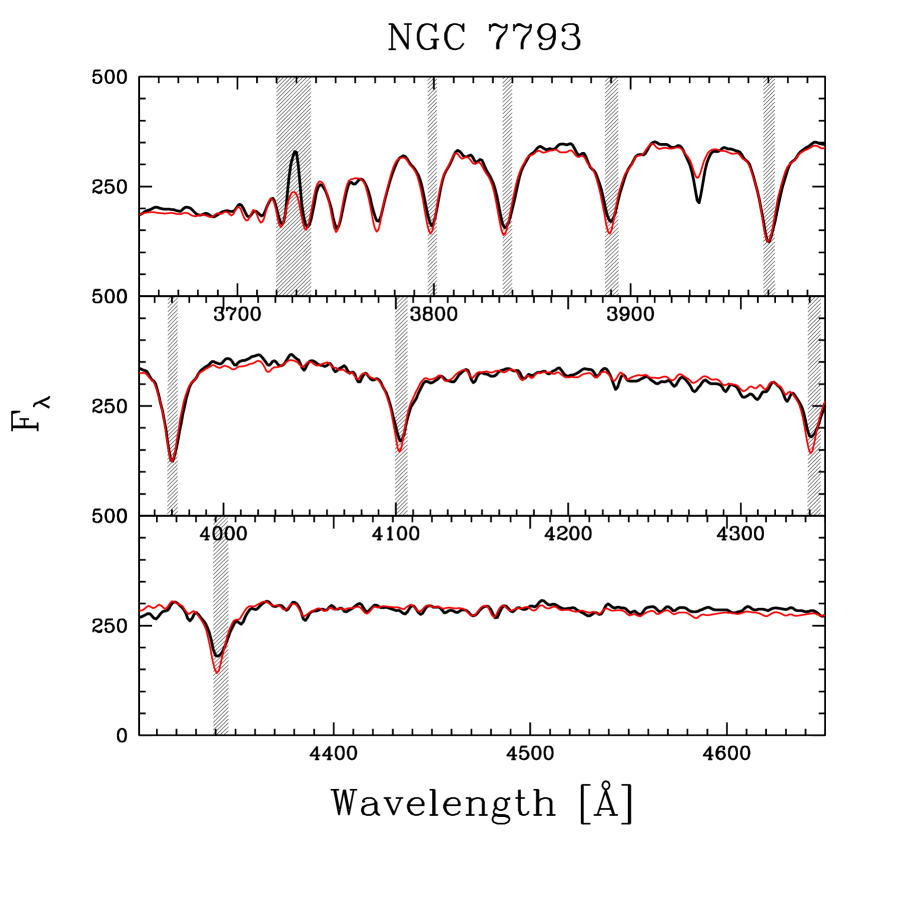
Figure 5: Best single age fit for NGC 7793 (thin dotted line, red in the online edition) compared to the observed spectrum (thick black line, arbitrary flux scale). Note that the Balmer and [OII] emission lines are excluded from the fit (shaded areas). Also note that the single age fit fails to fit the Ca K line at 3934 Å and smaller continuum features in the red. The panels have a scale with a small amount of overlap in wavelength (so the same absorption line is sometimes seen in multiple panels).

Figure 5 shows the observed spectrum of the nuclear region in NGC 7793 (which has the highest S/N of all observed objects), along with the SED of the best-fit single age population. In general, the fit is quite good and reproduces also small features of the observed spectrum. As the Balmer and [OII] emission lines are excluded from the fit, they do not influence the determined age. On the other hand, several characteristic features are not fit well. In the case of NGC 7793 this includes the Ca K line and the redmost range of the spectrum.

In summary, the age of the best fitting single age stellar population is robust with respect to the chosen metallicity and extinction. The age estimates agree well with those determined from the spectral indices, confirming that most clusters are ’young’, i.e. their age is much smaller than a Hubble time.

3.3 Fitting Composite Stellar Populations

There are different reasons to expect that the NC spectra are only poorly described by SSP models. First, some of the spectra actually represent an aperture that encompasses cluster light and disk light in similar amounts. Their spectra should therefore be better described by a mixture of differently aged stellar populations. Second, the M/L_I ratios derived from the dynamical modelling of Paper I are usually twice as high as those derived from the SSP fits, a discrepancy that is larger than the uncertainties. This can be interpreted as due to the presence of an older underlying population that has higher M/L and therefore is underrepresented in the observed spectrum. The younger population with lower M/L dominates the spectrum, though it may contribute only little to the mass. We therefore want to test if we can directly detect mixed stellar populations in the nuclear spectra. Ideally we would like to date the last burst of star formation as well as the oldest population in the spectrum.

As described at the beginning of Section 3, any composite star formation history can be described by a linear superposition of multiple bursts of star formation. The task to find the best linear weight for each SSP in the template set to fit the total spectrum is implemented in our software through the algorithm of Lawson and Hanson (1974). We thus generalize the code used in Section 3.2 to allow for composite populations with multiple ages. We use the same template library and the same emission line masks as for the SSP fitting. For the sake of a well-defined answer we reduce the number of available templates to one mean metallicity for all templates in one set and then fit once for each metallicity available. It would also be possible that every population, especially the young ones, could have a different extinction. We here however assume that one extinction is sufficient to describe all populations in each object.

For each object we then explore the $\chi^{2}$-surface for a wide range of metallicity and extinction, deriving the best fitting composite age fit at each point. Table 5 lists the M/L_I and mean luminosity weighted age in the $I$-band $\langle\tau_{I}\rangle$ of the best fit for every object together with the associated metallicity $Z$ and the extinction A_I.

To derive uncertainties on the parameters of interest, we follow the same approach as in Section 3.1, rescaling the errors (or $\chi^{2}$ surface) in each object to yield $\chi^{2}_{\mbox{best}}\approx N_{\mbox{DOF}}\approx 900$. The exact number is different for each spectrum, as different regions of the spectrum are clipped because of emission lines. Again as in Section 3.1, errors projected on a two parameter space can then be derived from iso-$\Delta\chi^{2}$ contours. It turns out in all cases that no other value of $Z$ yields a fit within $\Delta\chi^{2}$ = 29 of the best fit, which corresponds to the 99% confidence interval in 14 dimensions. We therefore take the uncertainty in $Z$ to be equal to half the step-size with which we sample the metallicity range; i.e., $\Delta Z\approx 0.2$ dex. For A_I the typical uncertainty is of order the step size, i.e. $\Delta\mbox{A}_{I}\approx 0.05$. Table 6 lists the mass-to-light ratio (M/L_I) and the mass fraction that each SSP contributes in the best fit. We here list mass fractions, though the fit determines light fractions. Both are related by the M/L_I given in the first column of Table 6. The mass weights directly imply a star formation rate over the age range that each SSP represents. Figure 7 shows cuts through the $\chi^{2}$ surface as a function of $Z$ and A_I for two objects, namely NGC 300 and NGC7418.

The derived M/L_I and $\langle\tau\rangle$ depend on a total of 16 parameters (14 template weights, metallicity and extinction). To derive meaningful error estimates one would have to cover the full 16-dimensional $\chi^{2}$ space. This is computationally too cumbersome and hard to interpret. We therefore will give a more empirical discussion of the significance of the results in the next Section.

3.4 Comparing the Different Approaches

We now compare the three different approaches used to derive mean ages, metallicities, extinction parameters and mass-to-light ratios for integrated SEDs of star clusters. In this discussion we will refer to the approach of Section 3.1 as the index method, to the approach of Section 3.2 as the SSP method and finally to the approach of Section 3.3 as the composite fit.

It is first noteworthy that although the model indices were measured on the exact same spectra that are used for the spectral fitting, the index method does seem to match significantly less well than the spectral fitting in the sense that the reduced $\chi^{2}$ of the best fitting model is in general larger by one order of magnitude. This can be mainly attributed to our neglect of templates with complicated star formation histories (SFH) when comparing the data with the model indices. While the SFHs of galaxies are conventionally taken to be decaying exponentials, we have no a priori knowledge on the functional form of the SFH of NCs. Additional problems arise because the index method purposefully relies on a very small wavelength range, to extract specific information from the spectrum - it compresses the information. However, a specific disturbance to this small wavelength range, e.g. emission lines, can lead to significant changes in the reliability of the method. Also the metallicity determinations will be affected by the fact that the available wavelength range does not grant us access to indices which do not depend on metal-abundance ratios. The spectral fitting on the other hand does use the full information content of the spectra and provides a means to correct for a disturbance in a small wavelength range by masking it from the fit (although it is still affected by the lack of models with varying abundance ratios). It is therefore the method of choice in the following discussion. Spectral fitting, however, does not allow to distinguish between the effects of different parameters easily, because the change of one parameter does not only affect a single feature in the spectrum but rather changes the whole SED. This interpretation problem will stay with us during the rest of this Section.

A comparison of Table 3, 4 and 5 shows that all three approaches agree and measure in general a subsolar metallicity. There are some outliers, namely NGC 2139 in the index method and the composite fit, and NGC 428 in the SSP fit. However, the case of NGC 7424 (see Figure 7) shows that our metallicity results may not be very robust for every single object. We therefore conclude that while we have evidence that the nuclei of bulge-less spirals have on average a slightly sub-solar metallicity ($\langle Z\rangle=0.015\pm 0.004$), the robustness of the metallicity measure for single objects remains uncertain. When looking for comparison values in the literature, we find the following values for NGC 300. Butler et al. (2004) measured a metallicity of 0.006 from color-magnitude diagrams for the stars in the disk of NGC 300. Individual stars in NGC 300 have also been targeted spectroscopically. Urbaneja et al. (2003) have measured metallicities of 0.006 and 0.02 for two stars in the outskirts and in the center of the galaxy respectively. Zaritsky, Kennicutt & Huchra (1994) have determined Oxygen abundances for HII regions in NGC 300 and NGC 7793. Assuming solar abundance ratios, we transfer these values to a value of $Z$, using

$$\log(\mbox{Z})=\log\mbox{Z}_{\odot}+[12+\log(O/H)]_{\mbox{gal}}-[12+\log(O/H)]_{\odot},$$ (4)

where we take $[12+\log(O/H)]_{\odot}=8.93$ and $Z_{\odot}=0.019$ (Anders & Grevesse, 1989). We thus obtain $Z=0.012\pm 0.01$ at r = 2.5 kpc for NGC300 and $Z=0.015\pm 0.03$ at r = 1.7 kpc for NGC7793. The $Z$ values we derive for our NCs are almost a factor of two lower. There might be several physical reasons for this discrepancy, as e.g. population gradients, differences between gas-phase and stellar metallicities, or non-solar abundance ratios, but the largest issue remains the systematic uncertainties of the various measurements.

Concerning extinction, it should be noted first that the continuum slope itself is a function of age and metallicity. Therefore, there is a trade-off between including an old population in the composite fit and applying a higher extinction to an SSP spectrum. While extinctions measured from SSPs therefore are almost certainly biased, the extinctions measured from the composite fit should be less influenced by systematic biases. For our data, an additional significant caveat exists in that we measure extinction over a very limited wavelength range. While age is quite insensitive to the derived extinction on such a small wavelength range (compare Section 3.2), the value of the extinction itself may not be well constrained. Extinctions inferred from the composite fit are generally lower than those from the SSP method, probably implying that in the SSP case the contribution from an old stellar population is substituted by the higher extinction correction. Of the two objects with highest extinctions, NGC 7418 also has a dust lane that is visible on the HST $I$-band image from B02. While the NC in NGC 428 is rather old and we would therefore expect it not to be surrounded by a lot of gas, the galaxy NGC 428 as a whole probably is a recent merger and is forming stars at a rather high rate (Smoker et al. 1996), implying a gas and dust reservoir to be present in this galaxy. The spectral indices shown in Figure 3 imply a significant amount of extinction for this object. Fairly low internal extinction has generally been measured in extreme late-types spirals from broad band colors (e.g. de Blok et al. 1995; Tully et al. 1998) and from spectroscopy (e.g. Roennback & Bergvall 1995). The last authors find a median A_V = 0.3 (A${}_{I}\approx$ 0.2) for their sample of blue low-surface brightness galaxies. Urbaneja et al. (2003) also determined extinctions for the two aforementioned single A giants in NGC 300 and found that “magnitudes and colors are consistent with almost no reddening for both stars”. While these literature results are not contradicting our findings, it should be noted that there is no reason why the nucleus should not have an extinction value of its own, possibly different from the rest of the galaxy.

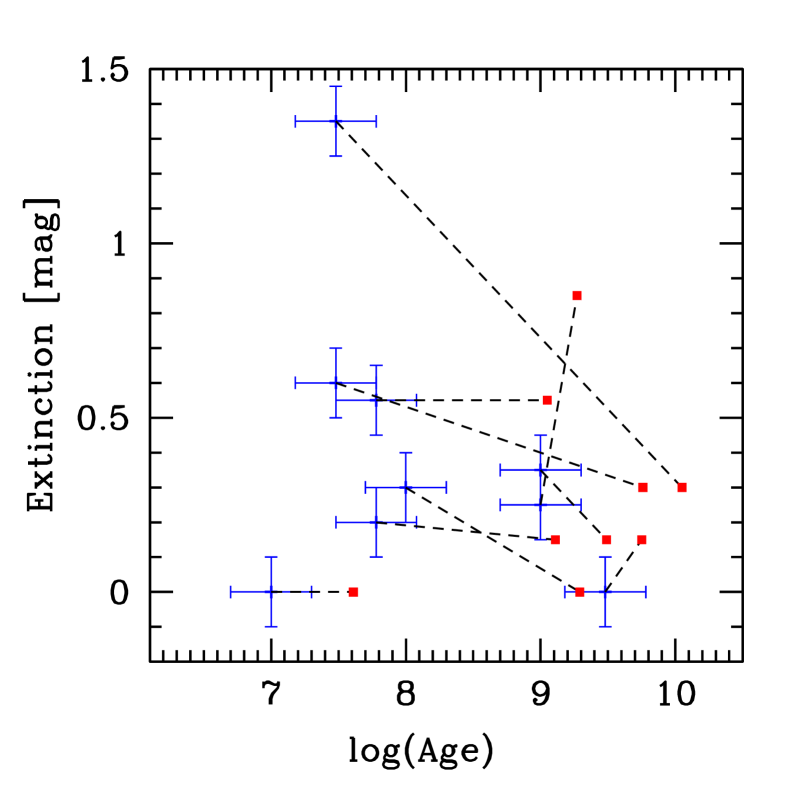
Figure 8: Comparison of the best fit values for the luminosity weighted mean age and extinction, as derived from the SSP method (plus sign with error bars - blue in the online edition) and the composite fit (filled square - red in the online edition). For each object the two symbols are joined with a dashed line.

Concerning age, the index method and the SSP method agree remarkably well within the uncertainties - despite all problems with the former. Thus, both suggest a distinction into two groups of nuclei: those that are $\lesssim 0.1$ Gyr (NGC 1042, NGC 1493, NGC 2139, NGC 7418, NGC 7424, NGC 7793) and those that are $\gtrsim 1$ Gyr (NGC 300, NGC 428, NGC 3423). Note that none of the inferred ages are nearly as high as those of the globular clusters of the Milky Way. Looking at the literature, Diaz et al. (1982) found that the spectrum of the nucleus of NGC 7793 is dominated by A or early F stars near the main sequence, in agreement with our findings. The mean luminosity-weighted age as derived in the $I$-band from the composite fit is older than the age inferred from the SSP fit in all nine cases. The division into 3 old and 6 young nuclei is however still valid in the sense that NGC 300, NGC 428 and NGC 3423 all have less than 3% of their mass in any population younger than 1 Gyr. Additionally, NGC 1042 needs to be added to this category. This is a particularly striking example of the trade-off between extinction and old population. For the 5 other spectra, the mass fraction of young populations is at least 10%. Figure 8 shows the different extinctions and mean luminosity weighted ages we obtain with the SSP method and the composite fit. This plot exhibits clearly the shift from young to old mean age that occurs when comparing the SSP to the composite fit.

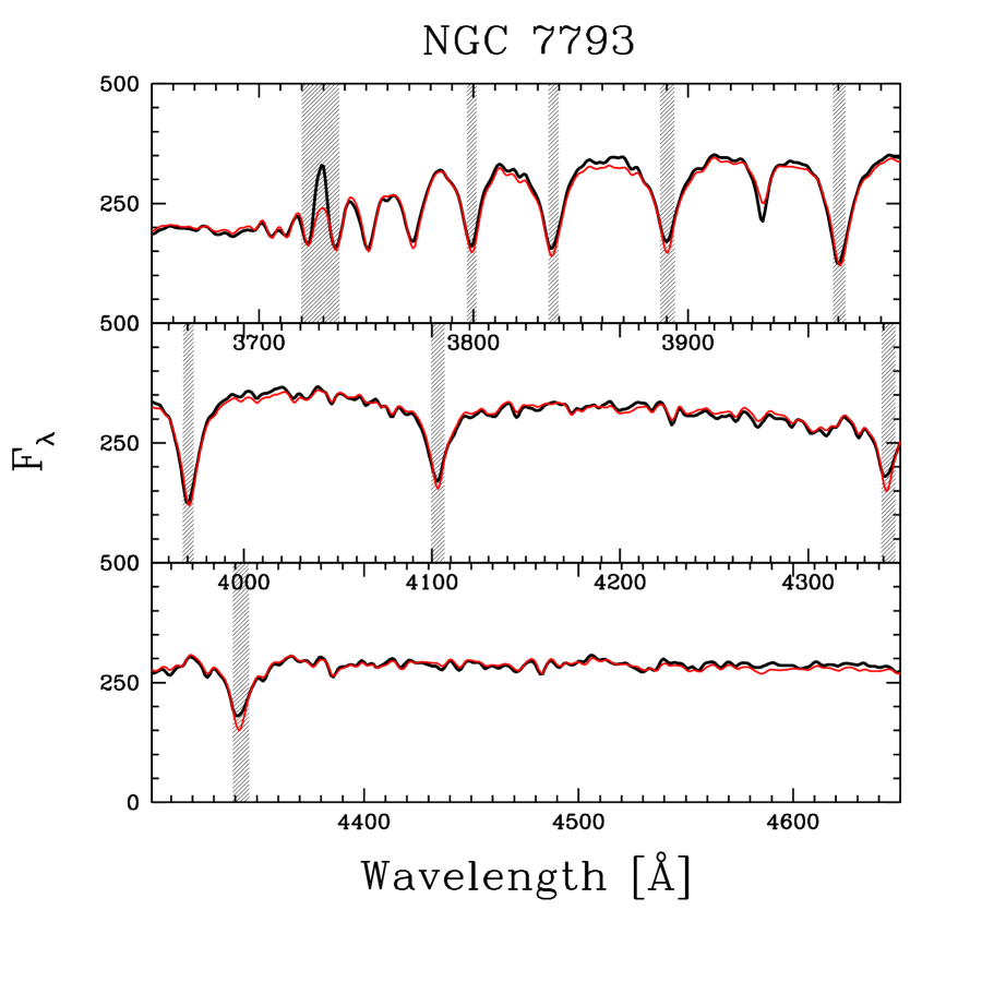
Figure 6: Best composite fit for NGC 7793 (thin, dotted line, red in the online edition) compared to the observed spectrum (thick line, arbitrary flux scale). Note that the Balmer and [OII] emission lines are excluded from the fit (shaded areas). Also note that the fit to the Ca K line at 3934 Å and the continuum in the red is improved, as compared to Figure 5. Note that the panels have a scale with a small amount of overlap in wavelength (so the same absorption line is sometimes seen in multiple panels).

Compared to the composite fit, only one of the SSP fits is statistically acceptable. Although this is not obvious from the example shown in Figures 5 and 6, $\chi^{2}$ increases by 40 % from the composite fit to the SSP fit on average over all nine spectra. A close inspection of the fits backs up these numbers. For example in NGC 7793 the fit to the Ca K line as well as to the reddest part of the spectrum is visibly improved in the composite fits. The one object where both $\chi^{2}$’s are comparable is NGC 2139, where a recent, strong burst of star formation probably swamps any light from older stellar populations.

However, there is yet another indication that the spectra are better represented by the composite fit. It was discussed earlier that the M/L_I ratios derived from the dynamical analysis should be matched by the population analysis. Figure 9 compares the mass-to-light ratios derived from the dynamical analysis to the mass-to-light ratios derived from the spectrum fits. The left panel shows the results obtained assuming a single-age population in the spectra. It is obvious that all but one object lie above the one to one relation, indicated as a straight line. This systematic offset (on average $\Delta$ M/L = 0.35 with an RMS scatter of 0.20) is reduced significantly if the mass-to-light ratio from the composite fit is plotted on the same graph (right, on average $\Delta$ M/L = -0.1) — albeit with a large RMS scatter of 0.58. Leaving out the ’outlier’ NGC 1042, these numbers come down to $\Delta$ M/L = 0.05 with a scatter of 0.28. Note here that this comparison is fully justified also in respect of the contamination from non-cluster light, because both values have been determined on spectra that were extracted on the same aperture.

3.5 The Youngest Population Component

Given the extensive set of 14 templates we fit to each spectrum in Section 3.3, it is difficult to fully explore the topology of the$\Delta\chi^{2}$ contours that encompass the acceptable solutions. Instead of exploring all co-variances, we will here ask a simpler question: how significant is the age of the youngest stellar population that contributes to the fit? More specifically, we explore the upper age bound on the youngest population component clearly required by the data. We derive this maximal age by subsequently eliminating more of the young components from the set of templates, re-fitting the data at each step. That is, we start from the best fit, obtained from a total of 14 template SSPs ranging in age from 1 Myr to 20 Gyr. We then omit first the youngest SSP age, leaving only 13 templates ranging from 3 Myr on. Then we repeat the fit omitting also the 3 Myr template, leaving only 12 templates from 6 Myr to 20 Gyr and so on. The maximum age of the youngest population age component is then defined as the age of the SSP whose omission increases $\chi^{2}$ significantly. The results of this procedure are shown in Figure 10 as $\Delta\chi^{2}$ plots. Although an exact definition of a confidence interval is non-trivial here (because of the change of degrees of freedom per fit), it is clear for all spectra which SSP’s omission changes $\Delta\chi^{2}$ drastically. Note that the fits cannot discriminate the age of the youngest population for quite a large interval in age in some cases! A conservative estimate of the last star formation age is given by the 99% confidence region in a 14 dimensional parameter space ($\Delta\chi^{2}<29$). Ages of the last SF burst ($\tau_{lb}$) derived this way are given in Table 8. Across the sample the mean age of the last star formation burst is then 34 Myr.

To derive a best estimate and a confidence region on the mass of this burst, one could think of varying the mass fraction of the last star formation burst. Technically, this would be done by subtracting a fraction of the light in the form of the SSP with the age derived for the last burst. However, we have seen above that the total mass of the population fit is subject to considerable scatter. This leads to a problem in the present case. Fitting after subtraction of a certain SSP may change the total M/L and thus $M_{\mbox{NC}}$ erratically. Indeed, increasing the fraction of light that a specified SSP contributes to the total blue luminosity of the object spectrum, does not necessarily imply increasing its mass fraction too. In the case of an increase of the total M/L, the mass fraction of the specified SSP may actually decrease. It turns out in practice that this is exactly what happens. Of course one can take at face value the mass fractions of the “last fitting model”, i.e., in the sequence of models as described above, the model that still includes the SSP with the age of the last burst. This model may be different from the best fit of Section 3.3. The mass fractions of the youngest SSP in that “last fitting model”, multiplied by the masses as derived in Paper I then yield mass estimates for the last burst – which should be regarded as indicative only. In order of ascending NGC number, we find the following log(M/M_⊙): NGC 300:4.5 - NGC 428:4.4 - NGC 1042:3.9 - NGC 1493:4.0 - NGC 2139:4.8 - NGC 3423:3.7 - NGC 7418:6.2 - NGC 7424:5.1 - NGC 7793:6.1 (mean log(M/M_⊙) = 5.5).

We applied a similar technique to test if we can derive meaningful results about the contribution of old SSPs to the fits. The most notable result is that in NGC 2139 even a modest contribution of 10% of the blue light from any population $\geq$ 0.1 Gyr is ruled out, in qualitative agreement with the low M/L_I derived dynamically. It is quite possible therefore that NGC 2139 contains a NC that is in the process of forming. However, it should be kept in mind that the light of this cluster is dominated by a very bright and young population with a low $M/L$. The best-fit SSP age is the youngest in our sample ($\log\tau=6.78$). Therefore, in this cluster it is particularly hard to detect an underlying older population. Even if an old (say $10^{10}$ yr) population contributed only one percent of the light in the cluster, it would still contribute as much mass as the young population. It is also striking that the NC in NGC 2139 is the only one, where we measure a super-solar metallicity. Taking this result at face value and admitting the cluster was forming right now, would require an unusually high metallicity for the gas that falls onto the cluster to form the stars.

3.6 How Important is the Disk Contamination?

Strictly speaking, we have up to now only shown that our observed spectra are generally best fit by multi-age populations. However, in view of the sometimes significant contribution by the light of the surrounding galaxy to the observed spectrum, we would like to know whether this is true for the NCs as well. In other words, is it possible that the NCs actually do have single-age populations, as is generally true for e.g. globular clusters and so-called super star clusters? If so, then our results can be explained only by the fact that we are observing a mixture of NC and disk light, and either of the following: (a) the NC and disk have different populations; or (b) the disk itself has a multi-age population, whereas the NC does not. In either case we would expect the spectra to be better described by an SSP in cases where the fraction of non-cluster-light (NCL) contamination is lower. We quantify the quality-of-fit difference between the SSP and the composite fit, namely

$$\Delta\chi^{2}=(\chi^{2}_{SSP}-\chi^{2}_{comp})\frac{N_{pix}-N_{free}}{\chi^{2}_{comp}},$$ (5)

where $N_{DoF}$ is the number of degrees of freedom and $N_{free}$ is the number of free parameters. In Figure 11 we plot this $\Delta\chi^{2}$ against the flux fraction of NCL from Table 1. This shows that less-disk-contaminated spectra are not more consistent with a single-age model. For comparison, the 99% confidence limit in a 14 dimensional $\chi^{2}$ space is shown as a dotted line. This test indicates that the presence of multi-age populations is not merely the result of disk-light contamination. We therefore conclude at this stage that the presence of mixed populations is a general feature not only of these galaxy centers, but also of the NCs. Of course this does not necessarily mean that the populations of the NC and the disk are the same. We further address this question in Section 4.

4 Comparison VLT/UVES vs. HST/STIS Spectra

Our population results describe the average stellar properties within an area of size $\sim 1^{\prime\prime}$, which is the spatial resolution of our VLT data. However, the NCs that we are interested in typically have effective radii $\leq 0\farcs 2$ (B04). As a result, in many of our spectra most of the observed light actually comes from the disk, and not from the cluster (Table 1). It is therefore possible that the population properties of the NCs are different from the average properties derived from the VLT spectra. To investigate this issue we also analyzed spectra obtained at higher spatial resolution. Such spectra are available for 4 of the 9 clusters in our sample from the Space Telescope Imaging Spectrograph (STIS) on the Hubble Space Telescope (HST). These spectra form part of our STIS spectroscopic survey of 40 NCs in both late-type and early-type spiral galaxies (HST programs GO-9070 and GO-9783; P.I. T. Böker). Preliminary results of this work for a subset of the sample were presented in Böker et al. (2003); a final analysis of the complete sample is presented in a separate paper (Rossa et al. 2006).

The STIS spectra were obtained with the G430L grating. They cover the wavelength range 2888.6–5703.2 Å with a pixel scale of $2.73$ Å. The spectra were obtained with a $0\farcs 2$-wide slit (52x0.2). The FWHM of the resulting line-spread function is $1.4$ pixels for a point source and $4.0$ pixels for a constant surface brightness extended source (Kim Quijano et al. 2003). The NCs are generally barely resolved at HST resolution, and fall between these extremes. For a $2.5$ pixel FWHM at 4000 Å the spectral resolution is $R=586$. The spatial pixel scale of the detector is $0\farcs 05$ per pixel. We extracted and co-added the central four rows from the pipeline reduced two-dimensional spectra. This yields for each galaxy a one-dimensional spectrum for a $0\farcs 2\times 0\farcs 2$ square aperture centered on the NC. This translates to $13.5$ pc $\times 13.5$pc at the mean distance to the galaxies. As done previously for the VLT/UVES spectra, an estimate for the (small) remaining contribution from the galaxy disk was subtracted from the STIS spectra.

Both the spectral resolution and the signal-to-noise ratio of the STIS spectra are worse than for the VLT spectra. Therefore, we do not repeat here for the STIS spectra the detailed analysis of metallicities and extinctions previously described for the VLT spectra. Instead, we kept the metallicity and extinction for each galaxy fixed to the previously derived values. We then used the exact same set of SSP templates of different ages to determine both the best single-age fit $\tau$, and the luminosity-weighted average age $\langle\tau\rangle$ (in the $I$-band) for the best composite-age population fit. For this analysis we resampled both the template and galaxy spectra to a common logarithmic scale of $138$ km s^-1 per pixel. We then determined the best-fitting redshift, dispersion, and population for each spectrum. The dispersion is a measure of the STIS instrumental resolution, and was found to be in the expected range for all galaxies analyzed. We used the wavelength range from 3539.7 Å to 5681.9 Å for the analysis. This extends further redward than the spectra used for the VLT analysis. For practical reasons we used independent software for the analysis of the STIS spectra, developed by one of us (RvdM), which differs in implementation from that described previously and used for the VLT spectra. This software is based on the van der Marel (1994) pixel fitting routine. Both codes solve the same $\chi^{2}$ minimization problem and we verified through extensive tests that both codes give consistent answers when applied to the same problem.

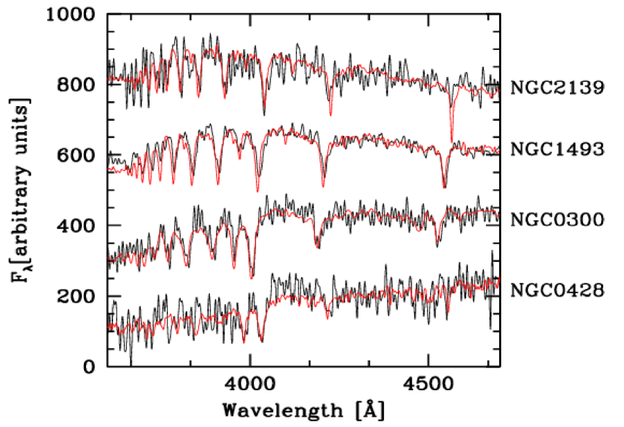
Figure 12: STIS spectra (black) of four NCs in the range from 3600 Å to 4700 Å overlaid with the VLT spectra (red). Note that despite the different apertures (0.2 $\arcsec$ vs. 1 $\arcsec$ respectively) the spectra are clearly similar. The spectra have been shifted arbitrarily in flux scale.

Figure 12 shows the STIS spectra and, overplotted, the VLT spectra. For this direct comparison the spectra were adjusted with respect to velocity (wavelength shift) and pseudoflux level. The good agreement between the spectra from totally different instruments also strengthens our confidence in the response correction we performed for both instruments. The composite age population fits for the STIS data are similarly good as for the VLT spectra. Table 7 compares the age results to those derived from the VLT spectra.

On average, the results for $\log_{10}\langle\tau\rangle$, the luminosity weighted mean age, are larger for the VLT spectra by $0.43\pm 0.51$ dex in the mean over the sample. For the simple SSP fit, $\log_{10}\tau$ is again larger for the VLT data than for the STIS data, in this case by $0.31\pm 0.11$ dex. These differences are comparable to the estimated uncertainty in the ages inferred from the SSP fits to the UVES spectra. They are much less than the typical age spread between the clusters. We do note that for NGC 1493 and NGC 2139 the VLT and STIS spectra give substantially different results for $\log_{10}\langle\tau\rangle$. This is not because the spectra or the fits are very different. Instead, the reason is that for spectra that are dominated by young light, the luminosity-weighted mean age $\langle\tau\rangle$ is very sensitive to even a small fraction of the light in a very old population. Small differences between the light fractions in the oldest populations (which are poorly constrained at the $\lesssim 10$% level) for the VLT and STIS fits generate large differences in $\log_{10}\langle\tau\rangle$ ($1.97$ dex for NGC 1493 and $-0.82$ dex for NGC 2139). By contrast, a statistic that is less sensitive to small amounts of light in the oldest population show much better agreement between VLT and STIS. For example, the difference in $\langle\log_{10}\tau\rangle$ (the luminosity-weighted average of $\log_{10}\tau$ for the composite fits) between the two samples is $0.31\pm 0.18$ dex. This has about three times less scatter than a comparison of $\log_{10}\langle\tau\rangle$.

The conclusions that we can draw from these comparisons are somewhat limited. Either way, it does not appear that the data provide evidence for the presence of strong population gradients between spatial resolutions of $0.2"$ (which mostly sample the NC) and $1.0"$ (which samples both the NC and the galaxy disk). Therefore, we believe that our VLT results provide a reliable characterization of the NC properties in our sample galaxies, despite the contamination from disk light.

5 Discussion

In summary, our extensive population analysis has shown that there is strong evidence that nuclear clusters have multiple-aged stellar populations. The average metallicity is somewhat sub-solar, but is higher that those of disk globulars in the Milky Way. The derived properties of the nine NCs in our sample are summarized in Table 8. The mean age $\log\,\langle\tau\rangle$ and derived metallicity $Z$ are taken from Section 3.3. We argued in Section 3.4 that these should be the determinations least influenced by systematic biases. The age of the most recent burst of star formation log($\tau_{lb})$ is taken from Section 3.5. We have not listed formal errors on these quantities, as the uncertainties are dominated by systematic and modelling uncertainties, as extensively discussed in Section 3. We give order of magnitude estimates in the footnotes to the Table. The masses log(M) in Table 8 are dynamical mass estimates, taken from Paper I. There masses were derived from a direct measurement of the velocity dispersion and careful dynamical modelling, which is much less prone to systematic problems than an analysis based on population synthesis models.

5.1 The Duty Cycle of Star Formation in NCs

The age of the last star formation burst in the NCs can be used to derive the duty cycle of star formation in the clusters, i.e. the fraction of time during which the clusters are actively forming stars. For each cluster we know that no sizable star formation occurred in the time since the last burst. So, each individual cluster was on a fraction $f^{k}_{on}=T_{\mbox{on}}/\tau^{k}_{lb}$ of the time, where $T_{\mbox{on}}$ is the typical duration of a star formation episode. Here $\tau^{k}_{lb}$ is the time since the last burst in cluster $k$ as taken from Table 8. All $n$ clusters together were on a fraction

$$f_{on}=\frac{nT_{\mbox{on}}}{\sum_{k=1}^{n}\tau_{lb}^{k}}$$ (6)

of the time, which is the current duty cycle. Weidner et al. (2004) argue that the typical formation timescale $T_{\mbox{on}}$ of massive star clusters is between $10^{6}$ and $10^{7}$ years. If we assume the typical duration of one star formation event is $10^{6}$ years, the duty cycle as derived from the nine clusters in our sample is 3 %. Assuming the typical duration of a burst is $10^{7}$ years yields a duty cycle of 30 %.

A useful comparison number that we will elaborate on in a future paper on emission line properties of the NCs is the number of spectra that show prominent emission lines that could be indicative of ongoing star formation. Remember, however, that the spectra sample more than just the NC light in most of the cases and we have at present no means to be sure whether the emission really comes from the cluster or from the surrounding disk. It also remains possible that low-luminosity AGN contribute to the observed emission line flux. Out of the nine spectra, three show no emission, five show prominent emission and one is, though clearly detected, not very strong. If one were to derive a duty cycle from these numbers, it thus turns out to be around 60 %. Though we may thus have overestimated the age of the last star formation burst, this only strengthens our conclusion that the centers of late-type spirals are regularly forming new stars.

It should be noted here that the relatively low average metallicities we derive are consistent with the recurrent star formation scenario. In fact the metallicity of a recurrently replenished closed box (i.e. no outflow of metals from feedback winds, but inflow of fresh gas) would be constant with time and depends only on the star formation efficiency and yield in the NC and on the metallicity of the infalling gas.

5.2 The Past Star Formation Rates of NCs

We also derive the star formation rate $<\mbox{SFR}>$ in the mean over eight of the nine clusters in our sample. NGC 7418, which has by far the largest mass of all NCs and also a sizable percentage of young stars, would contribute the bulk of the recent star formation to a simple average although it may not be typical for NCs as a class. We thus exclude it from the following averages. We follow two different approaches. First we simply assume that clusters build their mass $M_{NC}$ (as given in Table 8) continually over a Hubble time $t_{H}=13$ Gyr:

$$<\mbox{SFR}>_{1}=\sum_{k=1}^{8}\frac{M_{NC}^{k}}{8\times t_{H}}\approx 2\times 10^{-4}M_{\odot}/\mbox{yr}.$$ (7)

Second we can check if the SFR is constant over $t_{H}$ by comparing it to the SFR over the most recent $10^{8}$ years. We take the best fit mass weights $m^{k}_{l}$ of the composite population fits at face value. Here $k$ is an index running over the eight clusters and $l$ is an index running over the 14 SSP templates. We consider two broad age bins: the recently formed mass with age between $10^{6}$ and $10^{8}$ years and the old or “underlying” population with age between $3\times 10^{8}$ years and 20 Gyr. The mean star formation rate $<\mbox{SFR}>_{2}$ in the young bin is then

$$<\mbox{SFR}>_{2}=\sum_{k=1}^{8}\left(\frac{\sum_{l=1}^{7}m^{k}_{l}M_{NC}^{k}}{8\times 10^{8}\mbox{yr}}\right)=2.4\times 10^{-3}M_{\odot}/\mbox{yr},$$ (8)

where $l$ runs from the template with age $10^{6}$ years and index $l$ = 1 to the template with age $10^{8}$ years and index $l$ = 7.

We found in Section 3.5 that the star formation bursts are typically separated by $2\times 34$ Myr (the factor two arises because the probability to observe one object at any time between two bursts is constant with time). Thus in the mean over all objects the most likely point in time at which we observe is when half of the time between two bursts has elapsed since the last burst. The mass of stars that is formed per burst $M_{fpb}$ is then

$$M_{fpb}=<\mbox{SFR}>_{2}\times 2\times 34\mbox{Myr}=1.6\times 10^{5}M_{\odot}.$$ (9)

This number can be compared with the mean mass per burst derived in Section 3.5. Leaving out NGC 7418, one finds M = $1.9\times 10^{5}M_{\odot}$ for this comparison number. Each cluster has thus experienced of the order of 25 bursts in its lifetime.

As discussed in Section 3.4, the mass fractions of the populations in each cluster are subject to considerable scatter. Therefore the star formation rates we derive could be uncertain by up to a factor of 2. However $<\mbox{SFR}>_{2}$ is bigger than $<\mbox{SFR}>_{1}$ by one order of magnitude. At the current $<\mbox{SFR}>_{2}$ (leaving out NGC 7418), NCs need only be $\approx$ 2 Gyr old to build up their typical mass of $5\times 10^{6}$ M_⊙. Assuming that current star formation rates are typical for the whole existence of the clusters, would lead to the conclusion that NCs do not need to form in the very young universe. We already pointed out in Section 3.5 that the NC of NGC 2139 possibly contains no population older than 100 Myr. NGC 2139 is also the lightest of the clusters at a mass of only $8\times 10^{5}$ M_⊙ (one could speculate that this could be the typical mass at formation time for a NC). Note that the mass we derive as the mass formed per burst is close to the mass we derive for this NC. So it is possible that it formed just recently, i.e. around $10^{8}$ years ago.

On the other hand it should be remembered that the mass weights of the composite fits in Table 6 show that out of nine clusters, six formed more than 50% of their mass more than $10^{9.4}$ years ago. There is also no basis for the assumption that the star formation rate remains constant over time. Indeed, more massive clusters could attract more gas, therefore increasing their star formation rate over their lifetime. Finally, we are biased observationally to miss the very faintest, i.e. possibly older, NCs. Therefore we are possibly biased to higher SFRs.

5.3 Clues on the Formation Process?

As stated in the introduction, there is no obvious, compelling reason why the centers of late-type spirals should be conducive to the genesis of such massive, compact clusters. In standard star formation processes, the upper limit of the cluster mass distribution depends on the star formation rate in the sense that higher star formation rates lead to the formation of a larger number of clusters, which then sample further into the high-mass tail of the cluster mass distribution function (Larsen 2002). Star formation rates in late-type disks are in no way comparable to those of starburst galaxies like M82, where the formation of massive clusters has been observed (e.g. McCrady et al. 2003). Cluster formation in starburst galaxies is also expected to be a spatially random process, in clear contradiction to the observation that there is only one NC, which is located in the very nucleus of its host galaxy. It is thus highly unlikely that NCs form from such a standard cluster formation mode. Furthermore, though repetitive star formation in galactic nuclei has been predicted by e.g. Krügel & Tutukov (1993), these results are not directly applicable to the present case as their scenario includes the steep potential well of a bulge and spatial scales of up to 1 kpc, far in excess of the typical size of the NC.

A few authors have provided interesting first steps towards understanding the formation of NCs. Under the assumption of a singular gravitational potential, Milosavljevic (2004) has shown that the disks of late-type spirals can transport gas inwards at a rate of roughly $1\times 10^{-2}$ M_⊙/yr, which is sufficient to sustain the star formation rates we derive in the present paper. It remains however unclear, why the star formation should concentrate in a spatial region with a size of only 5 pc. Bekki et al. (2004) and Fellhauer et al. (2002) consider the case in which massive star clusters are formed from the merger of several recently formed “normal” star clusters under the influence of their own gravity. Typical initial conditions are adapted to regions of very high star formation activity, as this is the environment where it is most likely to find a sufficient number of star clusters (around 20) in a sufficiently small volume (a size of roughly 100 pc). The process can happen on a timescale of less than $10^{8}$ years if the initial conditions are right. If the process was to go much slower (more than a Gyr), the still distinct clusters in the process of merging should be visible in the HST images, which is not the case (compare B02). The effective radii they obtain from these simulations are between 10 and 50 pc. While this scenario could explain high masses, it thus generally fails to reproduce the small sizes and mixed populations of the observed NCs.

The origin of the nuclei of dE galaxies, which are possibly related to NCs, is generally attributed to two possible mechanisms, i.e. (a) the decay of the orbit of a pre-existing globular cluster toward the bottom of the galactic potential well, driven by dynamical friction, or (b) the in situ formation of a giant cluster from gas fallen to the center of the galaxy (see e.g. Durrell 1997). Dynamical friction timescales (larger than several Gyrs, see Milosavljevic 2004) are too long to account for the generally young ages of the NCs in late-type spirals. As a conjecture as for how NCs form, the following scenario would however fit all observed properties: Take a randomly forming star cluster in the very vicinity of the galaxy center (i.e. center of rotation and potential). Once formed, this cluster’s potential will itself be the minimum of the total galaxy’s potential (or it will tend to drift their because of dynamical friction). Thus the gas present in the disks of extremely late-type spirals will be accreted on the cluster. The gas can reach the center in a quiet, non-star forming mode because the surface density of the disk is so low. Thus the gas is only induced to form stars when falling into the proto-NC. It thus contributes to the high space density in the cluster. As a large fraction of the infalling gas will thus reach the NC, it can grow ever bigger. This scenario thus could explain the high masses, small radii and recurring star formation events in the clusters. It also describes in a natural way, why 25% of the late-type spirals lack a NC: simply because they have up to now lacked a suitable seed cluster. Whether this scenario can quantitatively explain the observed properties of NCs remains to be tested with detailed numerical simulations. It remains unclear in particular, how well the coincidence between NC and galaxy center can be accounted for.

6 Conclusions

We have presented results from a spectroscopic survey of the nuclear regions of late-type spiral galaxies, undertaken with VLT/UVES. We aimed to study the stellar population properties of the single, most luminous star cluster in the photometric center of the galaxy, which we call a nuclear star cluster. We used population synthesis models to derive mean luminosity weighted ages within the aperture of the extracted spectra. We found no evidence for strong radial age gradients between spatial resolutions of $0\farcs 2$ (which mostly sample the nuclear cluster, from HST/STIS data) and $1^{\prime\prime}$ (which samples both the nuclear cluster and the galaxy disk, from VLT/UVES data), implying that we can directly measure the stellar populations of the nuclear clusters. Fits using simple SSP models yield ages of the dominating population in the spectra that range between $1\times 10^{7}$, and $3\times 10^{9}$ years, and which are robust to the assumed metallicity or internal extinction. They are also consistent between two different approaches, namely either using Lick/IDS indices or directly fitting the spectrum with templates from the model over a spectral range of 1100Å.

We also fitted for the age composition of the clusters. These composite fits show that the luminosity weighted mean ages of nuclear clusters actually range from $4.1\times 10^{7}$ to $1.1\times 10^{10}$ years, with uncertainties of 0.3 dex. These ages are older than those suggested by SSP models. The average metallicity of nuclear clusters in late-type spirals is slightly sub-solar ($\langle Z\rangle=0.015$) but shows significant scatter. This is lower than for the nuclear regions in earlier-type galaxies (see e.g., Sarzi et al. 2005 and Rossa et al. 2006). The population synthesis model, however, does not at present cover varying abundance ratios, which limits the accuracy of this metallicity determination. While most of the clusters have moderate extinctions of 0.1 to 0.3 mags in the $I$-band, two out of nine clusters are extincted by 0.55 and 0.85 mag, respectively. The stellar mass-to-light ratios were well constrained from the composite-age fits and agree with the dynamical mass estimates. However a residual scatter remains due to the uncertain contributions of the oldest populations to the total light. We were also able to derive the age of the last star formation episode, which was in the mean over our nine sample clusters 34 Myr ago. All of the clusters experienced star formation in the last 100 Myr. For the clusters in our sample, an estimate for the mean star formation rate over the last 100 Myr is $<\mbox{SFR}>=2\times 10^{-3}M_{\odot}/{yr}$.

We have presented a number of independent arguments that point towards repetitive star formation in the nuclear clusters:

• The mean age of light dominating the clusters is $10^{8}$ years, which is much smaller than the age of the universe. Excluding the possibility that we live in special times, i.e. that all clusters happened to form recently, this can be explained convincingly in a repetitive scenario, as younger stellar populations have intrinsically lower mass-to-light ratio than older populations. Thus they mask the main mass of the cluster which resides in a significantly older, “underlying” population. It has to be kept in mind however that selection effects might bias us towards younger clusters as we only sample the brighter 2/3 of the luminosity range of the nuclear clusters.

• The measured spectral indices are consistent with a continuous star formation history and inconsistent with a single burst in most cases.

• Single-age fits to the spectra are significantly worse in a $\chi^{2}$ sense than the multi-component fits in all cases.

• The cluster mass-to-light ratios as derived from the single-age fits are not consistent with those derived from the dynamical modelling of Paper I, while those derived from the composite fits are.

The population fits and star formation rates show that nuclear clusters form stars onto the present day. A caveat remains, namely that some of the mixed populations that we see might be due to disk star contamination in the spectra. However we found no evidence for strong radial age gradients, hence no evidence for strong disk contamination.

Taking these results together with those from Paper I we have thus shown that nuclear star clusters are massive and dense star clusters that form stars recurrently until the present day. We also refer to the recent paper of Rossa et al. (2006) for a study on a larger sample of NCs, which finds results that are entirely consistent with ours. A detailed comparison between our two samples is also given in that paper. While nuclear clusters are dynamically and structurally similar to the most massive globular clusters and super-star-clusters, these results show that their star formation histories and populations are unique in the whole star cluster domain. It is almost inevitable to associate these unique properties with the location of the cluster in its host galaxy. It remains a challenging question to elucidate exactly how very late-type spirals manage to create their extreme property nuclei. In turn, our results make perhaps even more puzzling why other, structurally similar galaxies, seem to have no significant nuclear clusters at all (B04).

Figure 1: Reduced, response-corrected blue spectra of the nuclear regions ($\sim 1^{\prime\prime}$) of the nine galaxies in our sample. Mean stellar ages increase from top to bottom. The pseudo-flux scale and offset of each spectrum have been adjusted arbitrarily.

Figure 2: Dependence on age and metallicity of different spectral indices measurable in the UVES data as predicted from the BC03 models. Each line illustrates how the indices behave as the model age is varied, and the different lines correspond to different metallicities (solid $Z$=0.05, dotted $Z$=0.02, short dashed $Z$=0.008, long dashed $Z$=0.004). Note that the left five indices are good age indicators (though the Balmer indices are double valued, so require a further constraint for age measurements). The six indices on the right are more sensitive to metallicity, again in particular at old ages.

Figure 3: Key spectral indices measured for the nine spectra and compared to the predictions by population synthesis models. We here plot two age sensitive indices, D_n(4000) and H$\delta_{A}$. The tracks of SSP models are indicated as different lines, corresponding to different metallicities (solid $Z$=0.05, dotted $Z$=0.02, short dashed $Z$=0.008, long dashed $Z$=0.004); models with continuous star formation are represented as a shaded area (from Kauffmann et al. 2003). Note that many NCs do not match the locus of the SSP models, but have indices indicative of continuous or repeated star formation.

Figure 4: $\chi^{2}$ as a function of SSPs of different age, metallicity $Z$ and extinction A_I for the nuclear spectrum of NGC 7418. The upper panel shows $\chi^{2}$ as a function of log(age) for different values of $Z$ and A_I. Note that the best fit age is independent of the chosen metallicity or extinction. The dotted line is the minimum $\chi^{2}$. The lower panel shows in more detail that the best fit extinction is well defined in a $\chi^{2}$ sense. Here, we plot $\chi^{2}$ as a function of A_I for the values of $Z$ and age that correspond to the best fit. The dashed line corresponds to the 99% confidence limit.

Figure 7: Cuts through the $\chi^{2}$-surface as a function of metallicity and extinction for two objects, obtained by optimizing the possible composite age distribution at each point. Panels that would be empty because of high $\chi^{2}$ values have been omitted (compare Figure 4). Note that both quantities are well defined from the point of view of $\chi^{2}$ statistics for most objects as for NGC 300. The case of NGC 7424 however shows that metallicity might not be very robust for this method. The $\chi^{2}$ value of the best fit has been adjusted to correspond to the number of free parameters. The dotted line represents the 99% confidence interval in 14 dimensions, $\Delta\chi^{2}<29$.

Figure 9: Mass-to-light (M/L_I) ratios as derived by the dynamical analysis of Paper I against the M/L_I as derived from fitting SSPs to the blue spectra (left, Section 3.2) or from fitting composite stellar populations (right, Section 3.3). The line indicates a one-to-one relation. Note that the M/L_I values of the composite fit are a better match to the dynamically measured M/L_I than those from the SSP method.

Figure 10: $\Delta\chi^{2}$ as a function of the age of the youngest SSP in the template library for the composite fit. The dashed line shows the 99% confidence region in a 14 dimensional parameter space ($\Delta\chi^{2}<29$).

Figure 11: $\Delta\chi^{2}$ between SSP fit and composite fit against the fraction of non-cluster light, NCL, in the spectra. The absence of a correlation shows that the presence of composite populations is a general feature not only of these galaxy centers, but also of the NCs.

Table 1: Sample properties

Galaxy	Hubble	Distance	MI	Aperture	re	NCL
	type	[Mpc]		[$\arcsec$]	[$\arcsec$]	[%]
(1)	(2)	(3)	(4)	(5)	(6)	(7)
NGC 300	SAd	2.2	$-11.43$	1.09	0.272	0
NGC 428	SABm	16.1	$-13.15$	0.93	0.043	30
NGC 1042	SABcd	18.2	$-12.95$	0.93	0.022	81
NGC 1493	SBcd	11.4	$-11.43$	1.24	0.047	33
NGC 2139	SABcd	23.6	$-12.65$	1.24	0.090	89
NGC 3423	SAcd	14.6	$-11.84$	0.93	0.059	76
NGC 7418	SABcd	18.4	$-16.23$	1.40	0.140	18
NGC 7424	SABcd	10.9	$-11.41$	1.55	0.140	77
NGC 7793	SAd	3.3	$-13.64$	1.55	0.484	0

Note. — Cols. (1) and (2) Galaxy name and Hubble classification, as taken from NED. Col. (3) Distances were taken from B02, where they were calculated from the recession velocity (from LEDA, corrected for virgocentric infall) and assume H${}_{0}=\rm{70\,km\,s^{-1}\,Mpc^{-1}}$. Col. (4) Absolute magnitude of the NC as taken from B02. Col. (5) Width of the extraction aperture in spatial direction. Col. (6) and (7) Effective radius of the NC and contamination from galaxy light in percent, as derived in Paper I.

Table 2: Measured indices

NGC No.	0300	0428	1042	1493	2139	3423	7418	7424	7793
Dn(4000)	1.534 $\pm$ 0.005	1.85 $\pm$ 0.03	1.408 $\pm$ 0.008	1.231 $\pm$ 0.002	1.042 $\pm$ 0.005	1.632 $\pm$ 0.005	1.317 $\pm$ 0.005	1.223 $\pm$ 0.005	1.317 $\pm$ 0.005
B4000	1.369 $\pm$ 0.0056	1.57 $\pm$ 0.03	1.27 $\pm$ 0.01	1.130 $\pm$ 0.002	1.011 $\pm$ 0.006	1.483 $\pm$ 0.006	1.157 $\pm$ 0.006	1.112 $\pm$ 0.007	1.182 $\pm$ 0.001
H$\delta_{A}$	4.4 $\pm$ 0.2	2.7 $\pm$ 0.8	3.6 $\pm$ 0.3	5.84 $\pm$ 0.09	5.3 $\pm$ 0.3	1.9 $\pm$ 0.2	4.7 $\pm$ 0.2	6.4 $\pm$ 0.3	7.29 $\pm$ 0.03
Ca4227	0.6 $\pm$ 0.1	0.1 $\pm$ 0.4	0.8 $\pm$ 0.2	0.20 $\pm$ 0.05	0.0 $\pm$ 0.2	1.45 $\pm$ 0.09	0.3 $\pm$ 0.1	0.4 $\pm$ 0.1	0.45 $\pm$ 0.02
G4300	2.5 $\pm$ 0.2	1.6 $\pm$ 0.7	2.2 $\pm$ 0.4	0.1 $\pm$ 0.1	0.1 $\pm$ 0.4	3.7 $\pm$ 0.2	0.0 $\pm$ 0.3	-0.3 $\pm$ 0.3	0.23 $\pm$ 0.04
H$\gamma$	1.1 $\pm$ 0.2	0.0 $\pm$ 0.7	0.0 $\pm$ 0.3	4.0 $\pm$ 0.1	4.8 $\pm$ 0.3	-2.2 $\pm$ 0.2	2.6 $\pm$ 0.2	4.6 $\pm$ 0.3	4.88 $\pm$ 0.04
Fe4383	2.0 $\pm$ 0.2	1.6 $\pm$ 0.9	3.2 $\pm$ 0.5	0.3 $\pm$ 0.1	1.0 $\pm$ 0.5	4.5 $\pm$ 0.2	1.7 $\pm$ 0.4	1.4 $\pm$ 0.4	1.00 $\pm$ 0.06
Ca4455	1.0 $\pm$ 0.1	0.0 $\pm$ 0.4	1.2 $\pm$ 0.2	0.24 $\pm$ 0.07	1.4 $\pm$ 0.3	1.8 $\pm$ 0.1	1.1 $\pm$ 0.2	1.0 $\pm$ 0.2	0.52 $\pm$ 0.03
Fe4531	2.3 $\pm$ 0.2	2.2 $\pm$ 0.7	2.5 $\pm$ 0.4	1.4 $\pm$ 0.1	0.5 $\pm$ 0.5	2.5 $\pm$ 0.2	0.8 $\pm$ 0.3	1.1 $\pm$ 0.4	1.46 $\pm$ 0.05
CaII8542	2.9 $\pm$ 0.1	1.9 $\pm$ 0.3	3.7 $\pm$ 0.1	2.9 $\pm$ 0.2	2.5 $\pm$ 0.1	3.1 $\pm$ 0.2	3.1 $\pm$ 0.1	2.4 $\pm$ 0.2	3.4 $\pm$ 0.1
CaII8662	2.4 $\pm$ 0.1	2.3 $\pm$ 0.3	3.6 $\pm$ 0.1	3.1 $\pm$ 0.2	2.8 $\pm$ 0.1	2.2 $\pm$ 0.2	3.1 $\pm$ 0.1	2.4 $\pm$ 0.2	3.34 $\pm$ 0.09

Note. — The following values are obtained for the Balmer indices if no interpolation of the emission lines is performed.

NGC 1042: H$\delta_{A}$ = 3.3 $\pm$ 0.3, H$\gamma$ = -0.8 $\pm$ 0.4

NGC 7418: H$\delta_{A}$ = 4.4 $\pm$ 0.2, H$\gamma$ = 1.5 $\pm$ 0.2

NGC 7424: H$\delta_{A}$ = 6.3 $\pm$ 0.3, H$\gamma$ = 4.0 $\pm$ 0.3

Table 3: Ages and metallicities from absorption indices

Galaxy	$\chi^{2}$	log($\tau$)	$Z$
NGC  300	154	9.11${}_{-0.00}^{+0.10}$	0.004
NGC  428	4.2	9.36${}_{-0.26}^{+0.08}$	0.004 - 0.02
NGC 1042	225	8.00${}_{-1.00}^{+1.00}$	0.004 - 0.05
NGC 1493	69	7.74${}_{-0.05}^{+0.11}$	0.004
NGC 2139	6	7.30${}_{-0.19}^{+0.06}$	0.05
NGC 3423	194	9.39${}_{-0.24}^{+0.36}$	0.004 - 0.02
NGC 7418	75	7.70${}_{-0.21}^{+0.16}$	0.004
NGC 7424	1.8	7.81${}_{-0.05}^{+0.05}$	0.004
NGC 7793	1417	8.26${}_{-0.15}^{+0.65}$	0.004 - 0.008

Note. — NGC 7418 has two minima that are almost equally good fits, the other minimum is at log($\tau$) = 6.86${}_{-0.06}^{+0.05}$ and $Z$=0.008. As the coverage of the models in $Z$ is sparse, the uncertainties in metallicity are noted as two different possible values in some cases.

Table 4: Ages and metallicities from fitting SSPs

Galaxy	$\chi^{2}$	$Z$	AI	log($\tau$)	M/LI
NGC 300	4128	0.004	0.35	9.00	0.41
NGC 428	246	0.05	0.25	9.00	0.41
NGC 1042	1107	0.004	1.35	7.48	0.07
NGC 1493	4604	0.008	0.60	7.48	0.07
NGC 2139	741	0.008	0.00	7.00	0.02
NGC 3423	6519	0.004	0.00	9.48	0.87
NGC 7418	1509	0.004	0.55	7.78	0.10
NGC 7424	594	0.004	0.20	7.78	0.10
NGC 7793	34768	0.008	0.30	8.00	0.15

Table 5: Ages and metallicities from composite age fits

Galaxy	$\chi^{2}$	$Z$	AI	$\log\langle\tau_{I}\rangle$	M/LI
NGC 300	1248	0.004	0.15	9.49	0.64
NGC 428	189	0.02	0.85	9.27	0.60
NGC 1042	320	0.02	0.30	10.05	2.06
NGC 1493	3996	0.008	0.30	9.76	0.88
NGC 2139	739	0.05	0.00	7.61	0.08
NGC 3423	3956	0.008	0.15	9.75	1.12
NGC 7418	737	0.008	0.55	9.05	0.30
NGC 7424	365	0.008	0.15	9.11	0.31
NGC 7793	27281	0.008	0.00	9.29	0.47

Note. — There are N${}_{\mbox{DOF}}$ = N${}_{\mbox{pix}}-$N${}_{\mbox{param}}\approx 900$ degrees of freedom.

Table 6: Linear mass weights of contributing SSPs in the composite fit

							NGC
$\log$(age)	M/LI	300	428	1042	1493	2139	3423	7418	7424	7793
6.00	0.05	0.000	0.000	0.000	0.000	0.000	0.001	0.009	0.000	0.000
6.48	0.02	0.000	0.000	0.000	0.000	0.079	0.000	0.000	0.000	0.000
6.78	0.02	0.000	0.001	0.001	0.000	0.000	0.000	0.004	0.000	0.000
7.00	0.02	0.000	0.000	0.000	0.004	0.000	0.000	0.000	0.019	0.000
7.48	0.07	0.000	0.000	0.000	0.031	0.000	0.002	0.087	0.059	0.012
7.78	0.10	0.000	0.000	0.000	0.000	0.921	0.000	0.000	0.000	0.000
8.00	0.15	0.027	0.000	0.004	0.000	0.000	0.000	0.000	0.000	0.101
8.48	0.23	0.000	0.000	0.000	0.014	0.000	0.000	0.056	0.291	0.079
8.78	0.34	0.000	0.000	0.000	0.043	0.000	0.000	0.117	0.000	0.045
9.00	0.41	0.013	0.348	0.052	0.000	0.000	0.000	0.154	0.000	0.000
9.48	0.87	0.637	0.651	0.019	0.000	0.000	0.000	0.000	0.000	0.000
9.78	1.47	0.323	0.000	0.000	0.000	0.000	0.997	0.574	0.000	0.762
10.00	2.08	0.000	0.000	0.000	0.000	0.000	0.000	0.000	0.631	0.000
10.30	3.53	0.000	0.000	0.924	0.908	0.000	0.000	0.000	0.000	0.000

Note. — The mass weights are the fraction of the total stellar mass at the present time.

Table 7: Population Analysis Comparison VLT vs. STIS

Galaxy	$Z$	$A_{I}$	$\log_{10}\tau_{\rm VLT}$	$\log_{10}\tau_{\rm STIS}$	$Z$	$A_{I}$	$\log_{10}\langle\tau\rangle_{\rm VLT}$	$\log_{10}\langle\tau\rangle_{\rm STIS}$
(1)	(2)	(3)	(4)	(5)	(6)	(7)	(8)	(9)
NGC 300	0.004	0.35	9.00	8.48	0.004	0.15	9.49	9.50
NGC 428	0.05	0.25	9.00	8.78	0.02	0.85	9.27	8.70
NGC 1493	0.008	0.6	7.48	7.00	0.008	0.30	9.76	7.79
NGC 2139	0.008	0.0	7.00	7.00	0.05	0.0	7.61	8.43

Note. — Col. (1) lists the galaxy name. Cols. (2)–(4) list the results from SSP fits to the VLT data for the metallicity, $I$-band extinction, and age, respectively (from Table 4). Col. (5) list the results from SSP fits to the STIS spectra, with metallicity and $I$-band extinction fixed to the values inferred from the VLT data. Cols. (6)–(8) list the results from composite-age fits to the VLT data for the metallicity, $I$-band extinction, and luminosity-weighted mean age in the $I$-band, respectively (from Table 5). Col. (9) list the results from composite-age fits to the STIS data, with metallicity and $I$-band extinction fixed to the values inferred from the VLT data.

Table 8: Summary of properties

Galaxy	$\log\,\langle\tau\rangle$	$Z$	log($\tau_{lb})$	log(M) [M☉]
NGC 0300	9.49	0.004	8.00	$6.02\pm 0.24$
NGC 0428	9.27	0.02	7.48	$6.51\pm 0.14$
NGC 1042	10.05	0.02	7.00	$6.51\pm 0.21$
NGC 1493	9.76	0.008	7.00	$6.38\pm 0.14$
NGC 2139	7.61	0.05	6.48	$5.92\pm 0.20$
NGC 3423	9.75	0.008	7.00	$6.53\pm 0.14$
NGC 7418	9.05	0.008	7.00	$7.78\pm 0.19$
NGC 7424	9.11	0.008	7.48	$6.09\pm 0.14$
NGC 7793	9.29	0.008	8.00	$6.89\pm 0.14$

Note. — Typical uncertainties on the mean ages $\log\,\langle\tau\rangle$ are $\pm$ 0.3 dex. Typical uncertainties on the metallicity $Z$ and the age of the youngest stellar population log($\tau_{lb})$ are half the step-size with which we sample the metallicity and age range, i.e. $\Delta Z\approx 0.2$ dex and $\Delta$ log($\tau_{lb}$) $\approx$ 0.15 dex respectively.

References

- (1) Anders, E., & Grevesse, N. 1989, Geochim. Cosmochim. Acta, 53, 197
- (2) P. Ballester, O. Boitquin, A. Modigliani, S. Wolf 2001, “UVES pipeline and Quality Control User’s Manual”, http://www.eso.org/instruments/uves/
- (3) Bica, E., Claria, J. J., Piatti, A. E., & Bonatto, C. 1998, A&AS, 131, 483
- (4) Bekki, K., & Freeman, K. 2003, MNRAS, 346, L11
- (5) Bekki, K., Couch, W.J., Drinkwater, M.J., & Shioya, Y. 2004, AJ, 610, 13
- (6) Bekki, K., & Chiba, M. 2004, A&A, 417, 437
- (7) Böker, T., van der Marel, R. P., & Vacca, W. D. 1999, AJ, 118, 831
- (8) Böker, T., van der Marel, R. P., Mazzuca, L., Rix, H.-W., Rudnick, G., Ho, L. C., & Shields, J. C. 2001, AJ, 121, 1473
- (9) Böker, T., Laine, S., van der Marel, R. P., Sarzi, M., Rix, H.-W., Ho, L. C., & Shields, J. C. 2002, AJ, 123, 1389 (B02)
- (10) Böker, T., van der Marel, R. P., Gerssen, J., Walcher, C. J., Rix, H.-W., Shields, J. C., & Ho, L. C. 2003, SPIE, 4834, 57
- (11) Böker, T., Sarzi, M., McLaughlin, D. E., van der Marel, R. P., Rix, H.-W., Ho, L. C., & Shields, J. C. 2004, AJ, 127, 105 (B04)
- (12) Bruzual, G. & Charlot, S. 2003, MNRAS, 344, 1000 (BC03)
- (13) de Blok, W. J. G., van der Hulst, J. M., & Bothun, G. D. 1995, MNRAS, 274, 235
- (14) de Blok, W. J. G., McGaugh, S. S., & Rubin, V. C. 2001a, AJ, 122, 2396
- (15) de Blok, W. J. G., McGaugh, S. S., Bosma, A., & Rubin, V. C. 2001b, ApJ, 552, 23
- (16) Butler, D. J., Martinez-Delgado, D., & Brandner, W. 2004, AJ, 127, 1472
- (17) Carollo, C. M., Stiavelli, M., de Zeeuw, P.T., & Mack., J. 1997, AJ, 114, 2366
- (18) Carollo, C.M., Stiavelli, M., & Mack, J. 1998, AJ, 116, 68
- (19) Chabrier, G., 2001, ApJ, 554, 1274
- (20) Chabrier, G., 2002, ApJ, 567, 304
- (21) Chabrier, G., 2003a, ApJ, 586, L133
- (22) Chabrier, G., 2003b, PASP, 115, 763
- (23) Davidge, T. J., Rigaut, F., Doyon, R., & Crampton, D. 1997, AJ, 113, 985
- (24) Davidge, T. J. 2000, AJ, 119, 748
- (25) Diaz, A. I., Pagel, B. E. J., Edmunds, M. G., & Phillips, M. M. 1982, MNRAS, 201, 49
- (26) Durrell, P.R. 1997, AJ, 113, 531
- (27) Fellhauer, M., Baumgardt, H., Kroupa, P., & Spurzem, R. 2002, Celest. Mech. Dyn. Astron. 82, 113
- (28) Ferrarese, L., & Merritt. D. 2000, ApJ, 539, 9
- (29) Ferrarese, L., 2002, ApJ, 578, 90
- (30) Gallagher, J.S., Goad J.W., & Mould, J. 1982, ApJ, 263, 101
- (31) Gallimore, J. F., & Matthews, L. D. 2003, in: Active Galactic Nuclei: from Central Engine to Host Galaxy, ed.: S. Collin, F. Combes & I. Shlosman, ASP Conference Series, Vol. 290, p. 501.
- (32) Gebhardt, K. et al. 2000, ApJ, 539, L13
- (33) Gelatt, A. E., Hunter, D. A., & Gallagher, J. S. 2001, PASP, 113, 142
- (34) Genzel, R., & Eckart, A. 1998, in: The central regions of the Galaxy and galaxies, Proceedings of the 184th symposium of the International Astronomical Union, ed. Y. Sofue. (Dordrecht: Kluwer), p. 421
- (35) Gordon, K. D., Hanson, M. M., Clayton, G. C., Rieke, G. H. & Misselt, K. A. 1999, ApJ, 519, 165
- (36) Graham, A.W., Erwin, P., Caon, N., & Trujillo, I. 2001, ApJ, 563, L11
- (37) Häring, N., & Rix, H.-W. 2004, ApJ, 604, L89
- (38) Ho, L.C., & Filippenko V.P., 1996, ApJ, 472, 600
- (39) Johnson, H.M. 1961, ApJ, 133, 309
- (40) Kauffmann, G. et al. 2003, MNRAS, 341, 33
- (41) Kim Quijano, J., et al. 2003, STIS Instrument Handbook, Version 7.0, (Baltimore: STScI).
- (42) Kormendy, J., & McClure, R. D. 1993, AJ, 105, 1793
- (43) Krabbe, A. et al. 1995, ApJ, 447, L95
- (44) Kroupa P., 2001, MNRAS, 322, 231
- (45) Lauer, T.R., Faber, S.M., Ajhar, E. A., Grillmair, C.J., & Scowen, P.A. 1998, AJ, 116, 2263
- (46) Larsen, S.S. 2002, AJ, 124, 1393
- (47) Lawson, C.L., & Hanson, R.J., Solving least squares problems. Prentice-Hall Series in Automatic Computation, Englewood Cliffs: Prentice-Hall, 1974
- (48) Le Borgne, J.-F., Bruzual, G., Pello, R., Lancon, A., Rocca-Volmerange, B., Sanahuja, B., Schaerer, D., Soubiran, C., & Vilchez-Gomez, R. 2003, A&A, 402, 433
- (49) Le Borgne, D., Rocca-Volmerange, B., Prugniel, P., Lancon, A., Fioc, M., & Soubiran, C. 2004, A&A, 425, 881
- (50) Long, K. S., Charles, P. A., & Dubus, G. 2002, ApJ, 569, 204
- (51) MacArthur, L. A. 2005, ApJ, 623, 795
- (52) Marchesini, D., D’Onghia, E., Chincarini, G., Firmani, C., Conconi, P., Molinari, E., & Zacchei., A. 2002, ApJ, 575, 801
- (53) van der Marel, R.P. 1994, MNRAS, 270, 271
- (54) Matthews, L.D., & Gallagher, J.S. 1997, AJ, 114, 1899
- (55) Matthew, L.D., Gallagher, J.S. et al. 1999, AJ, 118, 208
- (56) Matthews, L. D., & Gallagher, J. S. 2002, ApJS, 141, 429
- (57) McCrady, N., Gilbert, A. M., & Graham, J. R. 2003, ApJ, 596, 240
- (58) Milosavljevic, M. 2004, ApJ, 605, 13
- (59) O’Connell, R.W. 1983, ApJ, 267, 80
- (60) Phillips, A. C., Illingworth, G. D., MacKenty, J. W., & Franx, M. 1996, AJ, 111, 1566
- (61) Krügel, E., & Tutukov, A. V. 1993, A&A, 275, 416
- (62) Rix, H.-W. & White, S. 1992, MNRAS, 254, 389
- (63) Roennback J., & Bergvall, N. 1995, A&A, 302, 353
- (64) Rossa J., van der Marel, R. P., Böker, T., Gerssen, J., Ho, L. C., Rix, H.-W., Shields, J. C., & Walcher, C. J. 2006, AJ, submitted
- (65) Sarzi, M., Rix, H.-W., Shields, J.C., Ho, L.C., Barth, A.J., Rudnick, G., Filippenko, A.V., & Sargent, W. L. W. 2005, ApJ, 628, 169
- (66) Schinnerer, E., Eckart, A., & Tacconi, L. J. 2001, ApJ, 549, 254
- (67) Smoker, J. V., Davies, R. D., & Axon, D. J. 1996, MNRAS, 281, 393
- (68) Stephens, A. W. & Frogel, J. A. 2002, AJ, 124, 2023
- (69) Thatte, N., Quirrenbach, A., Genzel, R., Maiolino, R., & Tecza, M. 1997, ApJ, 490, 238
- (70) Thomas, D., Maraston, C., & Bender, R. 2003, MNRAS, 339, 897
- (71) Trager, S.C., Worthey, G., Faber, S.M., Burstein, D., & Gonzalez, J.J. 1998, ApJS, 116, 1
- (72) Tully, R. B., Pierce, M. J., Huang, J.-S., Saunders, W, Verheijen, M. A. W., & Witchalls, P. L. 1998, AJ, 115, 2264
- (73) Urbaneja, M. A., Herrero, A., Bresolin, F., Kudritzki, R.-P., Gieren, W., & Puls, J. 2003, ApJ, 584, 73
- (74) Walcher, C.J., van der Marel, R.P., McLaughlin, D., Rix, H.-W., Böker, T., Häring, N., Ho, L.C., Sarzi, M., & Shields, J.C. 2005, ApJ, 618, 237 (Paper I)
- (75) Weidner, C., Kroupa, P., & Larsen, S.S. 2004, MNRAS, 350, 1503
- (76) Worthey, G. 1994, ApJS, 95, 107
- (77) Worthey, G., Faber, S. M., Gonzalez, J. J., & Burstein, D. 1994, ApJS, 94, 687
- (78) Worthey, G., & Ottaviani, D.L. 1997, ApJS, 111, 377
- (79) Zaritsky, D., Kennicutt, R. C., & Huchra, J. P. 1994, ApJ, 420 87