Lensing Effects on Gravitational Waves in a Clumpy Universe
—Effects of Inhomogeneity on the Distance-Redshift Relation—

Abstract

The distance-redshift relation determined by means of gravitational waves in the clumpy universe is simulated numerically by taking into account the effects of gravitational lensing. It is assumed that all of the matter in the universe takes the form of randomly distributed point masses, each of which has the identical mass $M_{L}$. Calculations are carried out in two extreme cases: $\lambda\gg GM_{L}/c^{2}$ and $\lambda\ll GM_{L}/c^{2}$, where $\lambda$ denotes the wavelength of gravitational waves. In the first case, the distance-redshift relation for the fully homogeneous and isotropic universe is reproduced with a small distance dispersion, whereas in the second case, the distance dispersion is larger. This result suggests that we might obtain information about the typical mass of lens objects through the distance-redshift relation gleaned through observation of gravitational waves of various wavelengths. In this paper, we show how to set limitations on the mass $M_{L}$ through the observation of gravitational waves in the clumpy universe model described above.

1 Introduction

Owing to recent developments of observational techniques, it is expected that detection of gravitational waves will be achieved in the near future. Laser interferometer gravitational wave detectors, such as the Tokyo Advanced Medium-Scale Antenna (TAMA-300), the Laser Interferometer Gravitational-Wave Observatory (LIGO), Variability of Irradiance and Gravity Oscillations (VIRGO) and GEO-600, are in operation, and other projects, such as the Large-scale Cryogenic Gravitational wave Telescope (LCGT), LIGO2, the Laser Interferometer Space Antenna (LISA), the Decihertz Interferometer Gravitational Wave Observatory (DECIGO; Seto et al. (2001)), and the Big Bang Observer (BBO), are in the planning stage. In preparation for future breakthroughs associated with these projects, it is useful to discuss the information provided by gravitational wave data. Here we focus on inhomogeneities of our universe that can be investigated with gravitational wave observations.

Many cosmological observations suggest that our universe is globally homogeneous and isotropic, in other words, that the time evolution of the global aspect is well approximated by the Friedmann-Lemaître(FL) cosmological model. However, our universe is locally inhomogeneous. The effects of these inhomogeneities on the evolution of our universe or on cosmological observations draw our attention as one of the most important issues in cosmology. However, it is difficult to directly observe the inhomogeneities with optical observations because most of the matter in our universe is not luminous. One useful means of obtaining information about aspects of inhomogeneities is to examine gravitational lensing. Gravitational and electromagnetic waves are subject to gravitational lensing effects caused by inhomogeneously distributed matter around their trajectories. Therefore, we may find features of inhomogeneities through both observational and theoretical studies of the gravitational lensing effects in astronomically significant situations.

There are various candidates for the dark matter such as weakly interacting massive particles (WIMPs) and massive compact halo objects(MACHOs). Several observations have been undertaken to constrain the mass density of compact objects, $\Omega_{\rm CO}$; direct searches for MACHOs in the Milky Way have been performed by the MACHO and EROS collaborations through microlensing surveys. The MACHO group (Alcock et al., 2000) group concluded that the most likely halo fraction in form of compact objects with masses in the range 0.1-1$M_{\odot}$ is of about 20%. The EROS team concluded that the objects in the mass range from $2\times 10^{-7}M_{\odot}$ to $1M_{\odot}$ cannot contribute more than 25% of the total halo (Afonso et al., 2003). However, the universal fraction of macroscopic dark matter could be significantly different from these local estimates. Millilensing tests of gamma-ray bursts derive a limit on $\Omega_{\rm CO}$ of $\Omega_{\rm CO}<0.1$ in the mass range from $10^{5}$ to $10^{9}M_{\odot}$ (Nemiroff et al., 2001). Multiple imaging searches in compact radio sources derive the limit on $\Omega_{\rm CO}$ as $\Omega_{\rm CO}\lesssim 0.013$ in the mass range from $10^{6}$ to $10^{8}M_{\odot}$ (Wilkinson et al., 2001). The mass range of these observational tests are limited, and thus other methods to investigate the mass fraction of macroscopic compact objects in wider mass range are needed.

In this paper, we show that it is possible to extract information about the properties of macroscopic compact objects from the observational data of gravitational waves by analyzing the gravitational lensing effects due to these compact objects. For this purpose, we consider an idealized model of the inhomogeneous universe which has the following properties. First, this model is a globally FL universe. Second, all of the matter takes the form of point masses, each of which has the identical mass $M_{L}$. Finally, the point masses are uniformly distributed.

One of the main targets of gravitational-wave astronomy is binary compact objects. Their gravitational waves have much longer wavelengths $(\lambda)$ than the optical, and furthermore, these are coherent. In typical optical observations, the wavelength $(\lambda\sim 1\mu{\rm m})$ might be much shorter than the Schwarzschild radii of lens objects. Thus, we usually analyze the gravitational lensing effects on electromagnetic waves by using geometrical optics. In contrast, we need wave optics for the gravitational lensing of gravitational waves, since the wavelength of gravitational waves may be comparable to or longer than the Schwarzschild radii of lens objects. For example, the wave-band of LISA is typically $10^{11}-10^{14}$ cm; a point mass of $10^{5}-10^{8}M_{\odot}$ has a Schwarzschild radius almost equal to the wavelengths within that wave-band. When we consider gravitational lensing effects on the gravitational waves with $GM_{L}/c^{2}\lesssim\lambda$, we have to take the wave effect  (Nakamura, 1998) into account. In fact, remarkable differences between the extreme cases $\lambda\gg GM_{L}/c^{2}$ and $\lambda\ll GM_{L}/c^{2}$ have already been reported (Takahashi & Nakamura, 2003).

In order to obtain information about uniformly distributed compact objects by investigating the gravitational lensing effects in observational data, we focus on the relation between the distance from the observer to the source of the gravitational waves and its redshift. The distance is determined using the information contained in the amplitudes of the gravitational waves from the so-called standard sirens (Holz & Hughes, 2005). Although there are several similar analyses using the optical observation of Type Ia supernovae (Holz & Linder, 2005), gravitational lensing effects on gravitational waves can add new information about the properties of the lensing compact objects to that obtained by optical observations, by virtue of the wave effect, through which we can gain an understanding of the typical mass and number density.

Here we assume that the redshift of each source is independently given by the observation of the electromagnetic counterpart (Kocsis et al., 2006) or the waveform of the gravitational waves (Markovic, 1993). The luminosity distance $d_{\rm l}$ from the observer to the source is given by the waveform of the gravitational waves, as follows (Schutz, 1986). Since the orbit of binary will be quickly circularized by a gravitational radiation reaction (Peters & Mathews, 1963; Peters, 1964), the effect of ellipticity is negligible when the emitted gravitational radiation becomes so strong that we can observe it. Then, the two wave modes emitted from a binary of two compact objects with masses $m_{1}$ and $m_{2}$ are given by

$$h_{+} = \frac{2\mathcal{M}_{\rm chirp}^{5/3}(\pi f)^{2/3}\cos(2\pi ft)}{d_{\rm l}}(\cos^{2}\theta+1),$$ (1)

$$h_{\times} = \frac{2\mathcal{M}_{\rm chirp}^{5/3}(\pi f)^{2/3}\sin(2\pi ft)}{d_{\rm l}}2\cos\theta,$$ (2)

where $f$ and $\theta$ are the frequency and the angle between the angular momentum vector of the binary and the line-of-sight, respectively, and $\mathcal{M}_{\rm chirp}$ is the redshifted chirp mass, defined by

$$\mathcal{M}_{\rm chirp}=(1+z)M_{\rm chirp}=(1+z)\frac{(m_{1}m_{2})^{3/5}}{(m_{1}+m_{2})^{1/5}}.$$ (3)

Assuming a circular orbit, we have

$$\frac{df}{dt}=\frac{96\pi^{8/3}}{5}f^{11/3}\mathcal{M}_{\rm chirp}^{5/3}.$$ (4)

Eliminating $\mathcal{M}_{\rm chirp}$ and $\theta$ from equations (1), (2), and (4), we can obtain $d_{\rm l}$ if there is no gravitational lensing effect on the gravitational waves. However, if the gravitational waves are gravitationally lensed, their wave forms are changed. The gravitational lensing effects may lead to an incorrect estimation of $d_{l}$, and thus we have to know how the gravitational lensing changes the waveforms of the gravitational waves.

This paper is organized as follows. In §2, the basic theory of gravitational lensing is introduced. We discuss the lensing probability in §3. Then we show the calculation method and results for the distance-redshift relation in §§4 and 5. Finally, §6 is devoted to the conclusions and summary. Throughout the paper, we adopt the unit of $G=c=1$.

2 Review of gravitational lensing

In this section, we introduce basic equations for gravitational lensing.

2.1 Geometrical optics

In the case of a point-mass lens with mass $M_{L}$, the bending angle vector $\hat{\mbox{\boldmath{$\alpha$}}}(\mbox{\boldmath{$\xi$}})$ is given by (Schneider et al., 1992)

$$\hat{\mbox{\boldmath{$\alpha$}}}(\mbox{\boldmath{$\xi$}})=4M_{L}\frac{\mbox{\boldmath{$\xi$}}}{|\mbox{\boldmath{$\xi$}}|^{2}},$$ (5)

where $\xi$ is the impact vector (see Fig. 1). For convenience, we consider the “straight” line $A$ from a source to the observer and define the intersection point of $A$ with the lens plane as the origin of the lens position $\zeta$ and the ray position $\gamma$. We note that, in general, the vector $\xi$ is not orthogonal to the line $A$. However, if the geometrically thin lens approximation is valid, we can regard the vectors $\xi$, $\zeta$, and $\gamma$ as parallel to each other (Schneider et al., 1992).

We define $D_{S}$, $D_{L}$, and $D_{LS}$ as the angular diameter distances from the observer to the source, from the observer to the lens, and from the lens to the source, respectively. Using simple trigonometry (see Fig. 1), we find the relation between the source position $\eta$ and $\xi$,

$$\mbox{\boldmath{$\eta$}}=\frac{D_{S}}{D_{L}}\mbox{\boldmath{$\xi$}}-D_{LS}\hat{\mbox{\boldmath{$\alpha$}}}(\mbox{\boldmath{$\xi$}}).$$ (6)

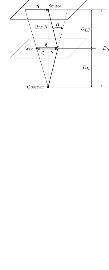
Figure 1: Geometry of gravitational lensing by a point-mass lens. The impact vector $\xi$ represents the relative position of a light ray on the lens plane to the lens position, and $\hat{\mbox{\boldmath{$\alpha$}}}$ is a vector whose norm is equal to the bending angle.

Equation (6) becomes

$$0=\frac{D_{S}}{D_{L}}\mbox{\boldmath{$\gamma$}}-D_{LS}\hat{\mbox{\boldmath{$\alpha$}}}(\mbox{\boldmath{$\gamma$}}-\mbox{\boldmath{$\zeta$}})$$ (7)

in terms of $\zeta$ and $\gamma$.

Here we introduce the dimensionless vectors defined by

$$\mbox{\boldmath{$x$}}=\frac{\mbox{\boldmath{$\xi$}}}{\xi_{0}}~{}~{}~{}~{}~{}{\rm and}~{}~{}~{}~{}~{}\mbox{\boldmath{$l$}}=\frac{\mbox{\boldmath{$\eta$}}}{\eta_{0}},$$ (8)

where $\xi_{0}$ is the Einstein radius given by

$$\xi_{0}=\sqrt{4M_{L}\frac{D_{L}D_{LS}}{D_{S}}}$$ (9)

and

$$\eta_{0}=\frac{D_{S}}{D_{L}}\xi_{0}.$$ (10)

From Figure 1, we find the relation

$$\mbox{\boldmath{$l$}}=-\frac{\mbox{\boldmath{$\zeta$}}}{\xi_{0}}.$$ (11)

The source will have two images at position $(\mbox{\boldmath{$x$}}_{+},\mbox{\boldmath{$x$}}_{-})$. Substituting equation (5) into equation (6) we find

$$x_{\pm}=\frac{1}{2}\left(\sqrt{l^{2}+4}\pm l\right),$$ (12)

where $x_{\pm}=|\mbox{\boldmath{$x$}}_{\pm}|$ and $l=|\mbox{\boldmath{$l$}}|$. The total magnification factor $\mu$ is given by

$$\mu=\left|\mu_{+}\right|+\left|\mu_{-}\right|=\left|\det\left(\frac{\partial\mbox{\boldmath{$l$}}}{\partial\mbox{\boldmath{$x$}}_{+}}\right)\right|+\left|\det\left(\frac{\partial\mbox{\boldmath{$l$}}}{\partial\mbox{\boldmath{$x$}}_{-}}\right)\right|=\frac{l^{2}+2}{l\sqrt{l^{2}+4}}.$$ (13)

2.2 Wave optics in gravitational lensing due to point mass lens

For simplicity, let us consider gravitational waves that propagate in asymptotically flat spacetime with the metric

$$ds^{2}=-(1+2U)dt^{2}+(1-2U)d\mbox{\boldmath{$r$}}^{2},$$ (14)

where $U$ is the gravitational potential and we assume $|U|\ll 1$. If the wavelength of the gravitational waves is much smaller than the typical curvature radius of the background spacetime, the equation for the gravitational waves is equivalent to that of scalar waves. Assuming monochromatic waves of an angular frequency $\omega$, we have (Peters, 1974)

$$\left(\nabla^{2}+\omega^{2}\right)\phi=4\omega^{2}U\phi.$$ (15)

For convenience, we introduce the amplification factor $F$ defined by

$$F=\frac{\phi^{L}(\omega)}{\phi(\omega)},$$ (16)

where $\phi$ is the plane wave with no lensing effects, and $\phi^{L}$ is the wave that is undergoing lensing effects. Here note that $\phi^{L}$ is no longer a plane wave, although it was initially. In the case of the point-mass lens with mass $M_{L}$, the gravitational potential is given by $U=-M_{L}/r$. Then we have the solution of equation (15) in the form

$$F(\omega;y)=\exp\left[\frac{\pi w}{4}+i\frac{w}{2}\ln\left(\frac{w}{2}\right)\right]\Gamma\left(1-\frac{i}{2}w\right)~{}_{1}F_{1}\left(\frac{i}{2}w,1;\frac{i}{2}wy^{2}\right),$$ (17)

where $\Gamma$ and $~{}_{1}F_{1}$ are the gamma function and the confluent hypergeometric function, respectively, and $w:=4\omega M_{L}$ (Peters, 1974). Since $\left|\nabla U\right|$ is much larger than the Hubble parameter of the universe, by replacing $\omega$ with $\omega(1+z_{L})$, we can use equation (17) in cosmological situations.

2.3 The Dyer-Roeder distance

In the clumpy universe model, the local geometry is inhomogeneous, but its global aspect might be well described by the FL universe whose metric is given by

$$ds^{2}=-dT^{2}+a^{2}(T)\left(\frac{dR^{2}}{1+KR^{2}}+R^{2}d\Omega^{2}\right),$$ (18)

where $K=1$, $0$, and $-1$, and $d\Omega^{2}$ is the round metric. However, the global aspect of the clumpy universe is a vague notion since we do not have a definite mathematical prescription to identify the global aspect of the locally inhomogeneous universe with the FL universe model. Therefore, the above FL universe is a fictitious background universe; hereafter, we will refer to this fictitious geometry (universe) as the “global geometry” (or universe). We assume that the global geometry is well approximated by that of the FL universe filled with dust and with a cosmological constant.

In the clumpy universe model, the distances $D_{L}$, $D_{S}$, and $D_{LS}$ in equation (6) or equation (7) are replaced by the Dyer-Roeder (DR) distances (Kantowski, 1969; Dyer & Roeder, 1973), which are the observed angular diameter distances if the gravitational waves propagate far from the point masses. The DR distance with smoothness parameter $\tilde{\alpha}=0$ (Schneider et al., 1992) in the global universe defined above is given by

$$D_{DR}(z_{1},z_{2})=\frac{1+z_{1}}{H_{0}}\int^{z_{2}}_{z_{1}}\frac{1}{(1+z)^{2}}\frac{dz}{\sqrt{\Omega_{\rm m0}(1+z)^{3}-\Omega_{\rm K0}(1+z)^{2}+\Omega_{\Lambda 0}}},$$ (19)

where $z_{1}$ and $z_{2}$ are the redshift of the observer and source, and $\Omega_{\rm m0}$, $H_{0}$, and $\Omega_{\rm\Lambda 0}$ are the present values of the total density parameter, Hubble parameter and normalized cosmological constant in the global universe, respectively, and $\Omega_{\rm K0}=\Omega_{\rm m0}+\Omega_{\Lambda 0}-1$. Hereafter, the subscript $0$ means the present value. Some further discussions of the properties of the DR distance are presented in Linder (1988), Seitz & Schneider (1994) , Kantowski (1998), and Sereno et al. (2001).

3 The distribution of point masses

In order for the clumpy universe to be the same as a homogeneous and isotropic universe from a global perspective, the point masses must be distributed uniformly. However, since there are no isometries of homogeneity and isotropy in the clumpy universe, the notion of “uniform distribution” cannot be introduced in a strict sense. Thus, we assume a uniform distribution of the point masses with respect to the global geometry represented by equation (18) in a manner consistent with the mass density of this global universe. This universe model is called “the on-average Friedmann universe.” The assumptions in this universe model are discussed in Seitz et al. (1994).

The comoving number density $\rho_{\rm n}$ of the point masses $M_{L}$ is given by

$$\rho_{\rm n}=\frac{a^{3}\rho}{M_{L}}=\frac{3\Omega_{\rm m0}H_{0}^{2}}{8\pi M_{L}},$$ (20)

where $\rho$ is the average mass density and we have set $a_{0}=1$. We consider a past light cone in the global universe. The vertex of this light cone is at the observer, at $R=0$ and $z=0$, and is parametrized by the redshift $z$ of its null geodesic generator. Then the comoving volume of a spherical shell bounded by $R(z)$ and $R=R(z+\Delta z)$ on this light cone is given by

$$\Delta V=4\pi R^{2}\frac{dR}{dz}\Delta z.$$ (21)

Therefore, the number of point masses in this shell is given by

$$\Delta N=\rho_{\rm n}\Delta V=\frac{3\Omega_{\rm m0}H_{0}^{2}}{2M_{L}}R^{2}\frac{dR}{dz}\Delta z,$$ (22)

where

$$\frac{dR}{dz}=\frac{1}{H_{0}}\sqrt{\frac{1+H_{0}^{2}\Omega_{K0}(1+z)^{2}D_{F}^{2}(z)}{\Omega_{\rm m0}(1+z)^{3}-\Omega_{K0}(1+z)^{2}+\Omega_{\Lambda 0}}},$$ (23)

where $D_{F}(z)$ is the angular diameter distance from the source of the redshift $z$ to the observer in the global universe, which is expressed as

$$D_{F}(z)=\left\{\begin{array}[]{ll}\displaystyle\frac{1}{H_{0}(1+z)}\frac{\sin X(z)}{\sqrt{\Omega_{\rm K0}}}&~{}~{}{\rm for}~{}~{}\Omega_{\rm K0}>0\\ \displaystyle\frac{1}{H_{0}(1+z)}Y(z)&~{}~{}{\rm for}~{}~{}\Omega_{\rm K0}=0\\ \displaystyle\frac{1}{H_{0}(1+z)}\frac{\sinh X(z)}{\sqrt{-\Omega_{\rm K0}}}&~{}~{}{\rm for}~{}~{}\Omega_{\rm K0}<0\end{array}\right.,$$ (24)

where

$$X(z)=\sqrt{\left|\Omega_{\rm K0}\right|}\int^{z}_{0}\frac{dz^{\prime}}{\sqrt{\Omega_{\rm m0}(1+z^{\prime})^{3}-\Omega_{\rm K0}(1+z^{\prime})^{2}+\Omega_{\Lambda 0}}},$$ (25)

$$Y(z)=\int^{z}_{0}\frac{dz^{\prime}}{\sqrt{\Omega_{\rm m0}(1+z^{\prime})^{3}-\Omega_{\rm K0}(1+z^{\prime})^{2}+\Omega_{\Lambda 0}}}.$$ (26)

The average number of point masses in the region $y<\zeta/\xi_{0}<y+\Delta y$ of this shell is given by

$$p(y,z)\Delta y=\frac{2\pi\xi_{0}^{2}y\Delta y}{4\pi a^{2}R^{2}}\Delta N.$$ (27)

Substituting equations (22) and (23) into equation (27) and using equation (9), we have

$$p(y,z)\Delta y=3H_{0}\Omega_{\rm m0}(1+z)^{2}\sqrt{\frac{1+H_{0}^{2}\Omega_{K0}(1+z)^{2}D_{F}^{2}(z)}{\Omega_{\rm m0}(1+z)^{3}-\Omega_{K0}(1+z)^{2}+\Omega_{\Lambda 0}}}$$

$$\hskip 199.16928pt\times\frac{D_{DR}(0,z)D_{DR}(z,z_{S})}{D_{DR}(0,z_{S})}y\Delta y\Delta z,$$ (28)

where $z_{S}$ is the redshift of the source and we have replaced each of distances in equation (9) with the DR distance. We find that $p(y,z)$ does not depend on $M_{L}$, and therefore the lensing probability for a given source does not depend on $M_{L}$.

We note that the assumption of the distribution of point masses given in equation (28) does not necessarily guarantee equality between the magnification in the global universe defined by

$$\mu_{F}:=\left(\frac{D_{DR}(0,z)}{D_{F}(z)}\right)^{2}$$ (29)

and the average magnification in the clumpy universe. Sevral previous works have discussed this issue  (Weinberg, 1976; Ellis et al., 1998; Claudel, 2000; Rose, 2001; Kibble & Lieu, 2005).

4 The long-wavelength case, $\lambda\gg M_{L}$

In the case of $\lambda\gg M_{L}$, the amplification factor $F(\omega(1+z_{L});y)$ is almost equal to unity (see Fig. 2) because of diffraction effects (Nakamura, 1998), and we have

$$\frac{|\phi_{L}-\phi|}{|\phi|}=|F(\omega(1+z_{L});y)-1|\ll 1.$$ (30)

Thus we assume that a wave $\phi$ can be treated as a spherical wave whose center is at the source during all stages of the propagation. Let us consider the situation in which $N$ point masses are located at $(z_{i},y_{i}),~{}i=1,\dots,N$,, where $i$ is the number assigned to each point mass in order of distance from the observer. If our assumption is valid, the wave $\phi$ is changed whenever it propagates near each point mass as

$$\phi\rightarrow F_{N}\phi\rightarrow F_{N}F_{N-1}\phi\rightarrow\cdots\rightarrow\prod_{i=1}^{N}F_{i}~{}\phi,$$ (31)

where

$$F_{i}=F\left(\omega\left(1+z_{i}\right);y_{i}\right).$$ (32)

Thus the observed amplitude $|\phi_{\rm obs}|$ is given by

$$|\phi_{\rm obs}|=\prod_{i=1}^{N}\left|F_{i}\right|\left|\phi\right|.$$ (33)

Then, the total amplification $\left|F_{\rm total}\right|$ is given by

$$\left|F_{\rm total}\right|=\prod_{i=1}^{N}\left|F_{i}\right|.$$ (34)

Figure 2: Amplification factor $F(\omega(1+z_{L});y)$ given in eq. (17) with replacement $\omega\rightarrow(1+z_{L})\omega$. We plot $\left|F-1\right|$ as a function of $y$ for three cases of $\lambda/M_{L}=10,10^{2}$, and $10^{3}$. The redshift of the source $z_{S}$ and of the lens $z_{L}$ are fixed for $z_{S}=2$ and $z_{L}=1$.

We randomly distribute point masses so that the distribution of those is consistent with equation (28). First, we divide the spherical region $z<z_{S}$ into $N$ concentric spherical shells, each of which is bounded by two spheres, $z=z_{i}-\Delta z/2$ and $z=z_{i}+\Delta z/2$. We take into account only the nearest lens in each shell. As described below, this procedure is valid for large numbers $N$, i.e., small $\Delta z$. We find from equation (28) that in the $i$th shell $z_{i}-\Delta z/2<z<z_{i}+\Delta z/2$, there is one point mass within the region $y\leq Y_{i}$ on average, where $Y_{i}$ is defined by

$$\int^{Y_{i}}_{0}p(y,z_{i})dy=1.$$ (35)

Then we randomly put a point mass within the region $y\leq Y_{i}$ in the $i$th shell. Here it is worth noting that $Y_{i}$ is an increasing function of $N$, so by setting $N$ large, we can take into account lenses far from the line $A$. Hence, in the limit of $N\rightarrow\infty$, we can all lenses take into account. The results do not depend on the value of $N$, if it is large enough  (see Figs. 3 and 4). In our calculations, we set $N$ sufficiently large.

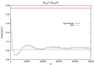
Figure 3: Observed distance $D_{\rm obs}$, depicted as a function of $N$ in the case of $\lambda/M_{L}=10^{6}$. The solid line represents the DR distance in the EdS universe. The dashed line represents the angluar diameter distance in the global universe.

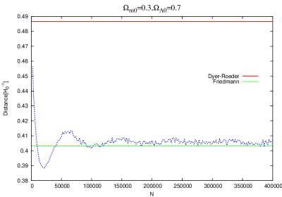
Figure 4: Same as in Fig. 3, but here the global geometry is given by the FL universe with $\Omega_{\lambda 0}=0.7$ and $\Omega_{\rm m0}=0.3$.

Calculating the total amplification factor $F_{\rm total}$, the observed distance is given by

$$D_{\rm obs}=\frac{D_{DR}(0,z_{S})}{|F_{\rm total}|}.$$ (36)

We have calculated $2000$ samples in two clumpy universe models, the globally Einstein-de Sitter (EdS) and globally FL universe with $\Omega_{\Lambda 0}=0.7$ and $\Omega_{\rm m0}=0.3$. The results are depicted in Figures 5 and 6, where we have randomly chosen the sources of the redshifts in the range $0<z_{S}\leq 2$.

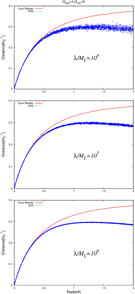
Figure 5: Distance-redshift relation of 2000 samples, depicted in the long-wavelength cases $\lambda/M_{L}\gg 1$. We have set $N=1,000+\lfloor 10,000\times z_{S}\rfloor$ in the cases of $\lambda/M_{L}=10^{4}$ and $10^{5}$, and $N=1,000+\lfloor 80,000\times z_{S}\rfloor$ in the case of $\lambda/M_{L}=10^{6}$. We have chosen the EdS universe, i.e., the FL model with $\Omega_{\Lambda 0}=0$ and $\Omega_{\rm m0}=1$, as a global universe. The solid line represents the DR distance in the EdS universe. The dashed line which is hidden behind the data points represents the angular diameter distance in the global universe.

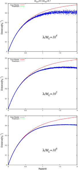
Figure 6: Same as in Fig. 5, but here the global geometry is given by the FL universe with $\Omega_{\Lambda 0}=0.7$ and $\Omega_{\rm m0}=0.3$.

The distance dispersion tends to vanish as $\lambda/M_{L}$ increases, and $D_{\rm obs}$ is almost equal to $D_{F}(z_{S})$ for sufficiently large $\lambda/M_{L}$  (see Figs. 7 and 8).

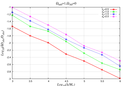
Figure 7: Relation between $\delta D_{\rm obs}/\left<D_{\rm obs}\right>$ and $\lambda/M_{L}$, where $\delta D_{\rm obs}$ and $\left<D_{\rm obs}\right>$ are the rms deviation and the average distance given by 100 samples of $D_{\rm obs}$ in each $\lambda/M_{L}$ and $z_{S}$.

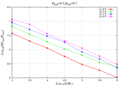
Figure 8: Same as in Fig. 7, but here the global geometry is given by the FL universe with $\Omega_{\Lambda 0}=0.7$ and $\Omega_{\rm m0}=0.3$.

As described in the next section, in the case of $\lambda/M_{L}\ll 1$, the dispersion is much larger than for $\lambda/M_{L}\gg 1$. It can be seen from Figures 7 and 8 that the distance dispersion does not sensitively depend on the value of $\Omega_{\rm m0}$, but become large as $z$ increase.

5 The short-wavelength case, $\lambda\ll M_{L}$

In the case of $\lambda\ll M_{L}$, the value of the amplification factor $F(\omega(1+z_{L});y)$ is much larger than unity for small values of $y$. Thus, we cannot use the linear approximation used in the previous section. Instead, here we adopt the geometrical optics approximation. We comment that it is difficult to resolve multiple images in the sky using gravitational wave detectors, because their angular resolution is $\sim 1^{\prime}$-$1^{\circ}$, much larger than the typical image separation. In geometrical optics, lensing does not change the wave form except for its amplitude (due to the magnification) and arrival time (due to the time delay) in each image. The observed waveform that is given by the superposition of waves from each image has undergone amplification and phase shift. In this paper, we assume stationary configurations, and the phase shift is not an observational variable. Therefore, we can observe only the amplitude of the superposed waves, and we cannot identify the signal as a superposed one.

5.1 The method of calculation

In order to calculate the amplification factor, we use the multiple lens-plane method (Schneider et al., 1992). We consider the “straight” line $A$ from a source to the observer, and we put $N$ lens planes between them so that the straight line $A$ intersects these lens planes vertically. The results do not depend on the value of $N$ if it is large enough; we set $N=10^{5}$ in our calculations.

In the same manner as in §4, we determine the redshifts $z_{i}$ and randomly situate a point mass $M_{L}$ within the region $y\leq Y_{i}$ on each lens plane $\Sigma_{i}$. In the case of $\lambda\gg M_{L}$, we have considered the lensing effects due to all point masses that we situate within the region $y\leq Y_{i}$. By contrast, in the case of $\lambda\ll M_{L}$, we can neglect the lensing effects due to the point masses that are far from the ray. Thus we take into account lensing effects due to the point masses in the region $y<y_{\rm max}$, where $y_{\rm max}$ is some positive constant smaller than $Y_{i}$. In other word, we take into account only a few lens planes in which a point mass is put within the region $y\leq y_{\rm max}$. Hereafter we denote the number of lens planes that we take into account as $N_{L}$. The validity of this procedure will be supported by the discussion of methods for determining an appropriate value of $y_{\rm max}$ in §5.2.

We denote the lens planes from the observer to the source as $\Sigma_{1},\Sigma_{2},\dots,\Sigma_{N_{L}}$. For convenience, we name the source plane $\Sigma_{N_{L}+1}$, which is also orthogonal to the line $A$. We define the intersection point of $A$ with $\Sigma_{i}$ as the origin of the lens position $\mbox{\boldmath{$\zeta$}}_{i}$ and the ray position $\mbox{\boldmath{$\gamma$}}_{i}$. Suppose lens positions $\mbox{\boldmath{$\zeta$}}_{i}~{}(i=1,\dots,N_{L})$ are given. Then once the ray position $\mbox{\boldmath{$\gamma$}}_{1}$ is given on the first lens plane $\Sigma_{1}$, the ray position $\mbox{\boldmath{$\gamma$}}_{j}$ is recursively given by

$$\mbox{\boldmath{$\gamma$}}_{j}=\frac{D_{j}}{D_{1}}\mbox{\boldmath{$\gamma$}}_{1}-\sum_{i\leq j-1}D_{ij}\hat{\mbox{\boldmath{$\alpha$}}}(\mbox{\boldmath{$\gamma$}}_{i}-\mbox{\boldmath{$\zeta$}}_{i})$$ (37)

on the $j$th lens plane $\Sigma_{j}$ $(j\leq N_{L}+1)$, where $D_{1}=D_{DR}(0,z_{1})$, $D_{j}=D_{DR}(0,z_{j})$, and $D_{ij}=D_{DR}(z_{i},z_{j})$. For later convenience, we specify the ray positions and the lens positions by the following dimensionless quantities:

$$\mbox{\boldmath{$u$}}_{i} := \frac{\mbox{\boldmath{$\gamma$}}_{i}}{D_{i}},$$ (38)

$$\mbox{\boldmath{$q$}}_{i} := \frac{\mbox{\boldmath{$\zeta$}}_{i}}{D_{i}}.$$ (39)

Then equation (37) becomes

$$\mbox{\boldmath{$u$}}_{j}=\mbox{\boldmath{$u$}}_{1}-\sum_{i\leq j-1}\beta_{ij}\mbox{\boldmath{$\alpha$}}(\mbox{\boldmath{$u$}}_{i}-\mbox{\boldmath{$q$}}_{i}),$$ (40)

where denoting $D_{1N_{L}+1}$ and $D_{iN_{L}+1}$ by $D_{S}$ and $D_{iS}$, respectively,

$$\beta_{ij}:=\frac{D_{ij}D_{S}}{D_{j}D_{iS}}$$ (41)

and

$$\mbox{\boldmath{$\alpha$}}(\mbox{\boldmath{$u$}}_{i}-\mbox{\boldmath{$q$}}_{i}):=\frac{D_{iS}}{D_{S}}\hat{\mbox{\boldmath{$\alpha$}}}(\mbox{\boldmath{$\gamma$}}_{i}-\mbox{\boldmath{$\zeta$}}_{i}).$$ (42)

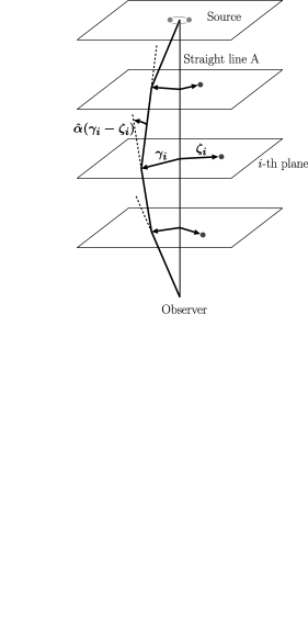
Figure 9: Definitions of the vectors $\mbox{\boldmath{$\alpha$}}_{j}$, $\mbox{\boldmath{$\zeta$}}_{j}$ and $\mbox{\boldmath{$\gamma$}}_{j}$.

Since more than one image appears in the present case, the amplification factor $F_{\rm total}$ is determined by both the interference of the rays corresponding to those images and the magnification of each ray due to the gravitational focusing effects. We specify a ray from the source to the observer by the ray position $\mbox{\boldmath{$u$}}_{1}=\mbox{\boldmath{$v$}}_{(p)}$ on the first lens plane $\Sigma_{1}$, where we have introduced the label $p$ to distinguish between the rays. The magnification $\mu_{(p)}$ for the ray $p$ is defined by

$$\mu_{(p)}=\frac{1}{\det\mathcal{A}_{(p)}},$$ (43)

where $\mathcal{A}_{(p)}$ is the Jacobian matrix of the lens mapping,

$$\mathcal{A}_{(p)} = \left.\frac{\partial\mbox{\boldmath{$u$}}_{N+1}}{\partial\mbox{\boldmath{$u$}}_{1}}\right|_{\mbox{\boldmath{$u$}}_{1}=\mbox{\boldmath{$v$}}_{(p)}}$$ (44)

$$= \mathcal{I}-\sum^{N}_{i=1}\beta_{i,N+1}\left.\frac{\partial\mbox{\boldmath{$\alpha$}}(\mbox{\boldmath{$u$}}_{i}-\mbox{\boldmath{$q$}}_{i})}{\partial\mbox{\boldmath{$u$}}_{i}}\frac{\partial\mbox{\boldmath{$u$}}_{i}}{\partial\mbox{\boldmath{$u$}}_{1}}\right|_{\mbox{\boldmath{$u$}}_{1}=\mbox{\boldmath{$v$}}_{(p)}}.$$

The amplification factor $F_{\rm total}$ is then given by

$$F_{\rm total}=\sum_{p}|\mu_{(p)}|^{1/2}\exp(i\theta_{(p)}),$$ (45)

where the phase $\theta_{(p)}$ is determined by the time delay $T_{(p)}$ relative to the ray that does not receive any lensing effect, and by the number of caustics $n_{(p)}$ on ray $p$ (Landau & Lifshitz, 1962), in the manner

$$\theta_{(p)}:=\omega T_{(p)}-\frac{\pi}{2}n_{(p)}.$$ (46)

The time delay $T_{(p)}$ is given by (Schneider et al., 1992)

$$T_{(p)}=\left.\sum_{i=1}^{N_{L}}(1+z_{i})\left\{\frac{D_{i}D_{i+1}}{2D_{i,i+1}}(\mbox{\boldmath{$u$}}_{i}-\mbox{\boldmath{$u$}}_{i+1})^{2}-4M_{L}\ln\left|\mbox{\boldmath{$u$}}_{i}-\mbox{\boldmath{$q$}}_{i}\right|\right\}\right|_{\mbox{\boldmath{$u$}}_{1}=\mbox{\boldmath{$v$}}_{(p)}},$$ (47)

and the number of caustics $n_{(p)}$ is give by

$$n_{(p)}=\sum_{i=1}^{N_{L}-1}n_{i(p)},$$ (48)

where $n_{i(p)}$ is the number of caustics between $\Sigma_{i}$ and $\Sigma_{i+1}$ on ray $p$ and its value is given by

$$n_{i(p)}=\left\{\begin{array}[]{l}\displaystyle 0~{}~{}{\rm for}~{}~{}\det\left(\frac{\partial\mbox{\boldmath{$u$}}_{i+1}}{\partial\mbox{\boldmath{$u$}}_{i}}\right)>0~{}~{}{\rm and}~{}~{}\textrm{tr}\left(\frac{\partial\mbox{\boldmath{$u$}}_{i+1}}{\partial\mbox{\boldmath{$u$}}_{i}}\right)>0\\ \displaystyle 1~{}~{}{\rm for}~{}~{}\det\left(\frac{\partial\mbox{\boldmath{$u$}}_{i+1}}{\partial\mbox{\boldmath{$u$}}_{i}}\right)<0\rule{0.0pt}{30.0pt}\\ \displaystyle 2~{}~{}{\rm for}~{}~{}\det\left(\frac{\partial\mbox{\boldmath{$u$}}_{i+1}}{\partial\mbox{\boldmath{$u$}}_{i}}\right)>0~{}~{}{\rm and}~{}~{}\textrm{tr}\left(\frac{\partial\mbox{\boldmath{$u$}}_{i+1}}{\partial\mbox{\boldmath{$u$}}_{i}}\right)<0\rule{0.0pt}{30.0pt}\end{array}\right..$$ (49)

The square of the absolute value of $F_{\rm total}$ is given by

$$|F_{\rm total}|^{2}=\sum_{p}|\mu_{(p)}|+\sum_{p\neq q}|\mu_{(p)}|^{1/2}|\mu_{(q)}|^{1/2}\cos\left(\theta_{(p)}-\theta_{(q)}\right).$$ (50)

The first term on the right-hand side of equation (50) represents the shear and focusing effect on the ray bundle, and the second term represents the interference effect (Nakamura & Deguchi, 1999).

Finally, we explain the method for finding rays from the source to the observer. If the lens positions $\mbox{\boldmath{$\zeta$}}_{i}$ ($i=1,...,N_{L}$) are given, the dimensionless ray position $\mbox{\boldmath{$u$}}_{N_{L}+1}$ on the source plane $\Sigma_{N_{L}+1}$ is completely determined by the ray position $\mbox{\boldmath{$u$}}_{1}$ on the first lens plane $\Sigma_{1}$;

$$\mbox{\boldmath{$u$}}_{N_{L}+1}=\mbox{\boldmath{$u$}}_{N_{L}+1}(\mbox{\boldmath{$u$}}_{1}).$$ (51)

Therefore, $\mbox{\boldmath{$v$}}_{(p)}$ is a root of the equation

$$\mbox{\boldmath{$u$}}_{N_{L}+1}(\mbox{\boldmath{$v$}}_{(p)})=0.$$ (52)

We solve equation (52) using the Newton-Raphson method, which requires initial estimates for the desired roots (Rauch, 1991). In order to find appropriate initial estimates, we consider a square region on the first lens plane $\Sigma_{1}$ whose center agrees with the intersection point of the straight line $A$ with $\Sigma_{1}$ (see Fig. 9) and with sides of length $2y_{\rm max}\xi_{01}$, where $\xi_{01}=\sqrt{4M_{L}D_{1}D_{1S}/D_{S}}$. In this square region, we place evenly spaced $n\times n$ grid points whose intervals are equal to $2y_{\rm max}\xi_{01}/n$. Substituting the position vector of each grid point to $\mbox{\boldmath{$u$}}_{1}$ on the right hand side of equation (51), we obtain the corresponding ray position $\mbox{\boldmath{$u$}}_{N_{L}+1}$ on the source plane. Then, we adopt the grid points which lead to

$$\frac{\gamma_{N_{L}+1}}{\sqrt{M_{L}D_{S}}}=\frac{D_{S}u_{N_{L}+1}}{\sqrt{M_{L}D_{S}}}<1$$ (53)

as the initial estimates of the Newton-Raphson method.

In practice, the interval between the grid points must be finite for the numerical calculations, so we may fail to find initial estimates that lead to some solutions $\mbox{\boldmath{$v$}}_{(p)}$. However, the magnification factors $\left|\mu_{(p)}\right|$ of such solutions are so small that the contributions to $\left|F_{\rm total}\right|$ will be negligible. In order to see this, let us consider the inverse map of equation (51). The inverse image of $S$ on the first lens plane consists of more than one connected region since multiple images of the source appear due to the lensing effects. If a grid point is contained in one of the connected regions, the grid point is found as an initial estimate by imposing the above criterion given by (53). If there is no grid point in a connected region due to its smallness, we cannot find initial estimates for the solution $\mbox{\boldmath{$v$}}_{(p)}$ included in the connected region and cannot find the solution $\mbox{\boldmath{$v$}}_{(p)}$ itself. Here we should note that the magnification factor associated with a root obtained from initial estimates contained in a connected region is almost proportional to the area of the connected region divided by the area of $S$. Therefore the magnification factor associated with the root we have failed to find will be small. For every initial estimate, we obtain the roots $\mbox{\boldmath{$v$}}_{(p)}$. However, these roots do not necessarily differ; the different initial estimates may lead to an identical root. Therefore, in order to prevent multiple counting, we have to take paths that differ from each other.

5.2 Determination of numerical parameters

We determine appropriate numerical values of $n$ and $y_{\rm max}$ to find all solutions $\mbox{\boldmath{$v$}}_{(p)}$ of equation (52) whose magnification factors $\left|\mu_{(p)}\right|$ significantly contribute to $\left|F_{\rm total}\right|$. If we fail to find such solutions, we underestimate the total flux that emanates from the source to the observer. Hence, this is a very important task. Since the interference effect is not important for our present purpose, we neglect it for simplicity. Then the total flux is proportional to the magnification $\mu$, defined by

$$\mu=\sum_{p}\left|\mu_{(p)}\right|.$$ (54)

If we increase the values of $n$ and $y_{\rm max}$, the magnification $\mu$ will approach the maximum value $\mu_{\rm max}$. We should determine the values of $n$ and $y_{\rm max}$ so that the magnification $\mu$ satisfies $\mu\simeq\mu_{\rm max}$. Since the lens distribution is determined using pseudorandom numbers, the magnification $\mu$ necessarily has a stochastic nature, and therefore we have to consider the ensemble average of $\mu$.

First, we set the source redshift $z_{S}$ to be $2$ and numerically generate samples of lens distributions with numbers much larger than 20,000. Then, with the parameters $y_{\rm max}$ and $n$ fixed, we calculate lens mappings to obtain the magnification $\mu$ for each lens distribution and construct an ensemble composed of 20,000 samples of $\mu$. This procedure is repeated to construct ensembles for various values of parameters $y_{\rm max}$ and $n$.

We denote one of the ensembles by $\cal{E}$, and further denote the ensemble average of a quantity $Q(\mu)$ related the magnification $\mu$ in $\cal{E}$ by $\left<Q\right>_{\cal{E}}$. The reader might think that $\left<\mu\right>_{\cal E}$ will approach $\mu_{\rm max}$ in the limit of large $y_{\rm max}$ and $n$, and thus we might be able to choose the parameters $y_{\rm max}$ and $n$ so that $\left<\mu\right>_{\cal E}$ sufficiently converges to some value that will be equal to $\mu_{\rm max}$. However this is not the case, for the following reason. As shown in §5.3, our numerical simulations imply that the probability $P(\mu)d\mu$ that the received magnification is in the range $(\mu,\mu+d\mu)$ is proportional to $\mu^{-3}$ for sufficiently large $\mu$. Therefore the second moment of the magnification $\left<\mu^{2}\right>$, defined by

$$\left<\mu^{2}\right>\equiv\int_{0}^{\infty}\mu^{2}P(\mu)d\mu$$ (55)

will diverge. This implies that the law of large numbers fails, or in other words, $\left<\mu\right>_{\cal{E}}$ cannot approximate the true average value $\left<\mu\right>$ even if the number of samples in the ensemble $\cal{E}$ is much larger than unity  (Paczyński, 1986; Holz & Wald, 1998; Rauch, 1991). Thus $\left<\mu\right>_{\cal{E}}$ cannot be a criterion for determining whether the values of the parameters $y_{\rm max}$ and $n$ are valid.

To obtain the criterion for determining validity of the choices of $y_{\rm max}$ and $n$, here we set an upper threshold $\mu_{\rm u}$ on $\mu$, and replace the magnification of samples in $\cal{E}$ by $\mu_{\rm u}$, if those are larger than $\mu_{\rm u}$. We denote the ensemble obtained by this procedure as $\hat{\cal E}$. The probability distribution of the samples in the ensemble $\hat{\cal E}$ will be well approximated by

$$\hat{P}(\mu)=\theta(\mu_{\rm u}-\mu)P(\mu)+\delta(\mu-\mu_{\rm u})\int^{\infty}_{\mu_{\rm u}}P(\bar{\mu})d\bar{\mu}$$ (56)

if $y_{\rm max}$ and $n$ are large enough, where $\theta(z)$ is a Heaviside’s step function, and $\delta(z)$ is a Dirac delta function. Then we expect

$$\left<\mu\right>_{\hat{\cal E}}\simeq\int^{\infty}_{0}\mu\hat{P}(\mu)d\mu.$$ (57)

We use $\left<\mu\right>_{\hat{\cal E}}$ as a criterion for the validity of the ensemble $\cal{E}$.

The relation between $\left<\mu\right>_{\hat{\cal E}}$ and the numerical parameters $y_{\rm max}$ and $n$ is depicted in Figures 10 and 11, where we have set $\mu_{\rm u}=100$. The value of $\left<\mu\right>_{\hat{\cal E}}$ almost converges to the maximum values at $y_{\rm max}=5,n=500$. In the case where the numerical parameters $y_{\rm max}$ and $n$ are not sufficiently large, there are lens distributions $(z_{i},y_{i})$ in which we cannot find any image. We exclude such cases as errors. In Table 1 we list the number of such errors appearing as we collected $20,000$ samples. Taking these results into account, hereafter we set $y_{\rm max}=5$ and $n=500$.

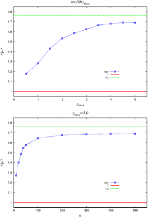
Figure 10: Ensemble average of magnification factor $\left<\mu\right>_{\hat{\varepsilon}}$, depicted as a function of the numerical parameters $n$ and $y_{\rm max}$. We have set $z_{S}=2$ and chosen the EdS universe as a global universe. The dashed horizontal line represent the value of $\mu_{F}$.

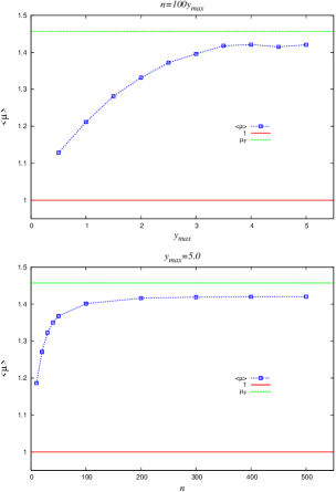
Figure 11: Same as in Fig. 10, but here the global geometry is given by the FL universe with $\Omega_{\Lambda 0}=0.7,~{}\Omega_{{\rm m}0}=0.3$.

Table 1: Number of errors in which we cannot find any image of the calculation for Figures 10 and 11 is given here.

$\Omega_{\Lambda 0}=0,\Omega_{\rm m0}=1$				$\Omega_{\Lambda 0}=0.7,\Omega_{\rm m0}=0.3$
$n=100\times y_{\rm max}$		$y_{\rm max}=5$		$n=100\times y_{\rm max}$		$y_{\rm max}=5$
$y_{\rm max}$	error	$n$	error	$y_{\rm max}$	error	$n$	error
$0.5$	$12$	$10$	$11791$	$0.5$	$6$	$10$	$8495$
$1.0$	$0$	$20$	$1294$	$1.0$	$0$	$20$	$864$
$1.5$	$0$	$30$	$290$	$1.5$	$0$	$30$	$168$
$2.0$	$0$	$40$	$83$	$2.0$	$0$	$40$	$61$
$2.5$	$0$	$50$	$34$	$2.5$	$0$	$50$	$22$
$3.0$	$0$	$100$	$2$	$3.0$	$0$	$100$	$1$
$3.5$	$0$	$200$	$1$	$3.5$	$0$	$200$	$0$
$4.0$	$0$	$300$	$0$	$4.0$	$0$	$300$	$0$
$4.5$	$0$	$400$	$0$	$4.5$	$0$	$400$	$0$
$5.0$	$0$	$500$	$0$	$5.0$	$0$	$500$	$0$

In our results, the value of $\left<\mu\right>_{\hat{\cal E}}$ is smaller than the magnification in the global universe $\mu_{F}$. Here it should be noted that $\left<\mu\right>_{\hat{\cal E}}$ is not an observable quantity in the gravitational wave observations, since we can observe the only amplitude of superposed waves, although it is observable in optical observations, e.g., the observation of Type Ia supernovae. As mentioned in §3, several works have discussed the equality between $\left<\mu\right>$ and $\mu_{F}$  (Weinberg, 1976; Ellis et al., 1998; Claudel, 2000; Rose, 2001; Kibble & Lieu, 2005). However, in practical sense, $\left<\mu\right>$ is not an observable quantity and thus $\left<\mu\right>_{\cal E}$ might be more important. We will discuss this issue in connection with the optical observation elsewhere.

5.3 Numerical results

The distance-redshift relation of $2,000$ samples is plotted in Figures 12 and 13. The probability distribution functions $P_{\rm a}(\left|F\right|^{2})$ in several source redshifts are depicted in Figures 14 and 15. The results do not depend on the value of $\lambda/M_{L}$ if it is much smaller than unity. In the case of $P_{\rm a}(|F|^{2})$, the gradient in the high-amplification tail is more gradual than $|F|^{-6}$, whereas it is approximately proportional to $|F|^{6}$ in the low-amplification tail (see Figs. 14 and 15). For comparison, we show the distance-redshift relation for incoherent waves  (see Figs. 16 and 17) and the probability distribution function of the magnification $P_{\rm m}(\mu)$  (see Figs. 18 and 19). The probability of receiving an extremely high magnification is very small for each ray. Therefore, if a ray is highly magnified, it comes from only one lens and the lens is located near the line of sight. In this case, we find

$$\mu\propto y^{-1}~{}~{}~{}{\rm for}~{}~{}~{}y\rightarrow 0$$ (58)

from equation (13). Hence, using equation (28), we find

$$P_{\rm m}(\mu)\propto p\left(y(\mu),z\right)\frac{dy}{d\mu}\propto\mu^{-3}.$$ (59)

We can see the consistent results in Figures 18 and 19.

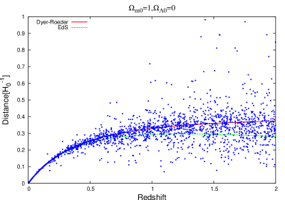
Figure 12: Distance-redshift relation in the case of short wavelength $\lambda\ll M_{L}$. The global geometry is given by the EdS universe. We have numerically generated $2,000$ samples but we cannot plot all of the data points in this figure, since some samples have distances too large to plot within the frame. The DR distance is depicted by the solid line and the angular diameter distance in the global universe is represented by the dashed line.

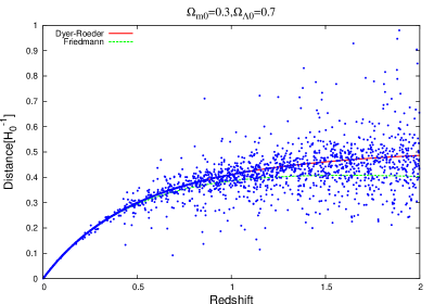
Figure 13: Same as in Fig. 12, but here the global geometry is given by the FL universe with $\Omega_{\Lambda 0}=0.7,\Omega_{\rm m0}=0.3$.

Figure 14: Probability distribution functions $P_{\rm a}(\left|F\right|^{2})$ in several source redshifts. The global geometry is given by the EdS universe. We have numerically generated $100,000$ samples for each $z_{S}$.

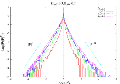
Figure 15: Same as in Fig. 12, but here the global geometry is given by the FL universe with $\Omega_{\Lambda 0}=0.7,\Omega_{\rm m0}=0.3$.

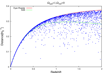
Figure 16: Distance-redshift relation in the case of incoherent waves with short wavelength $\lambda\ll M_{L}$. We have numerically generated 2000 samples, taking into account only the focusing effect generated by the first term on the right-hand side of eq. (50). The DR distance is depicted by the solid line and the angular diameter distance in the global universe is represented by the dashed line.

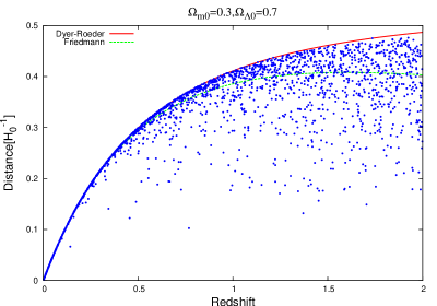
Figure 17: Same as in Fig. 16, but here the global geometry is given by the FL universe with $\Omega_{\Lambda 0}=0.7,\Omega_{\rm m0}=0.3$.

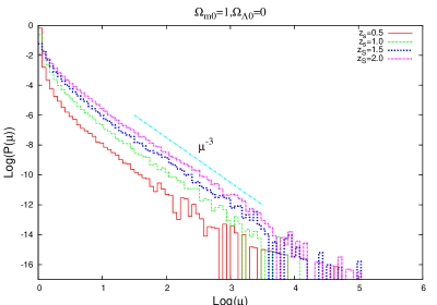
Figure 18: Probability distribution functions $P_{\rm m}(\mu)$ in several source redshifts. The global geometry is given by the EdS universe. We have numerically generated $100,000$ samples for each $z_{S}$.

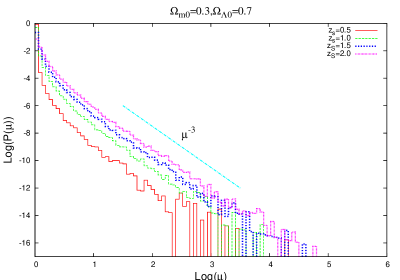
Figure 19: Same as in Fig. 12, but here the global geometry is given by the FL universe with $\Omega_{\Lambda 0}=0.7,\Omega_{\rm m0}=0.3$.

The distance dispersion is much larger than for long wavelengths, $\lambda\gg M_{L}$. The magnification of the amplitude comes from both the focusing and the interference effects, whereas the demagnification comes only from the interference effect. In contrast to the long-wavelength case, very large magnifications due to the focusing effect are possible for $\lambda\ll M_{L}$, because there is no significant diffraction. As already mentioned, the first term on the right-hand side of equation (50) includes the shear and focusing effects on the ray bundle, which can also be found in the case of incoherent waves (Holz & Wald, 1998), and these effects necessarily cause magnification of the amplitude (see Figs. 16 and 17). By contrast, since the second term on the right-hand side of equation (50) can take either sign, the amplitude can be strongly demagnified, i.e., $\left|F_{\rm total}\right|<1$. Thus very large demagnifications are also possible for short wavelengths, $\lambda\ll M_{L}$. As the result, the distance determined by the gravitational waves can grow longer than the DR distance. This is a peculiar nature of coherent waves.

Here we evaluate the distance dispersion that could be obtained by the data provided by gravitational waves if our universe is well described by the present clumpy mass distribution model. For this purpose, we have to take a detection limit for weak events into account. Let us consider the observation of $1\mathrm{Hz}$ gravitational waves emitted by neutron star-neutron star binaries that have the characteristic amplitude $h_{c}$, given by

$$h_{c}=9.88\times 10^{-24}(1+z_{S})^{5/6}\left(\frac{d_{\rm l}}{10\mathrm{Gpc}}\right)^{-1}\times\left\{\begin{array}[]{l}\frac{1}{2}\left(\cos^{2}\theta+1\right)\\ \cos\theta\end{array}\right.,$$ (60)

where $\theta$ and $d_{\rm l}$ are the inclination angle and luminosity distance of the binary (Hawking & Israel, 1989), respectively, and we have set the chirp mass of the binary to $1.2M_{\odot}$. The luminosity distance determined by lensed gravitational waves is given by $(1+z_{S})^{2}D_{DR}(0,z_{S})/\left|F_{\rm total}\right|$. Assuming the planed sensitivity of DECIGO (Seto et al., 2001), we set the detection limit as

$$h_{c}>10^{-23}.$$ (61)

Randomly choosing the inclination angle $\theta$, we numerically generate $20,000$ samples of $h_{c}$ for each source redshift and then select those that satisfy equation (61). We denote the number of detectable samples as $N_{\rm det}$. Results are shown in Tables 2 and 3 and Figures 20 and 21. The distance dispersion $\delta D_{\rm obs}$ is much larger than the estimate obtained by assuming a weak gravitational field for density perturbation  (Takahashi, 2006). This is because Takahashi (2006) assumed a linear approximation for the lensed waveform even in the short wavelength limit. Furthermore, he considered the density perturbation as the inhomogeneity, but in this paper we consider all the matter in the universe to be the point masses, which is a more extreme inhomogeneous model.

Table 2: Average distance $\left<D_{\rm obs}\right>$ and distance dispersion $\delta D_{\rm obs}$ for each source redshift, for EdS universe. The global geometry is given by the EdS universe. We have calculated the amplification factors $\left|F_{\rm total}\right|$ of $20,000$ samples for each redshift.

$z_{S}$	$N_{\rm det}$	$\delta D_{\rm obs}[H_{0}^{-1}]$	$\delta D_{\rm obs}/\left<D_{\rm obs}\right>$	$\left<D_{\rm obs}\right>[H_{0}^{-1}]$	$D_{DR}[H_{0}^{-1}]$	$D_{F}[H_{0}^{-1}]$
0.25	9339	1.16$\times 10^{-2}$	6.81%	1.71$\times 10^{-1}$	1.71$\times 10^{-1}$	1.69$\times 10^{-1}$
0.5	8863	3.23$\times 10^{-2}$	12.8%	2.53$\times 10^{-1}$	2.55$\times 10^{-1}$	2.45$\times 10^{-1}$
0.75	8450	5.01$\times 10^{-2}$	16.9%	2.96$\times 10^{-1}$	3.01$\times 10^{-1}$	2.79$\times 10^{-1}$
1.0	8066	6.48$\times 10^{-2}$	20.3%	3.18$\times 10^{-1}$	3.29$\times 10^{-1}$	2.93$\times 10^{-1}$
1.25	7673	7.56$\times 10^{-2}$	22.9%	3.29$\times 10^{-1}$	3.47$\times 10^{-1}$	2.96$\times 10^{-1}$
1.5	7221	8.35$\times 10^{-2}$	25.2%	3.31$\times 10^{-1}$	3.60$\times 10^{-1}$	2.94$\times 10^{-1}$
1.75	6780	8.88$\times 10^{-2}$	27.1%	3.28$\times 10^{-1}$	3.68$\times 10^{-1}$	2.89$\times 10^{-1}$
2.0	6113	9.32$\times 10^{-2}$	29.0%	3.22$\times 10^{-1}$	3.74$\times 10^{-1}$	2.82$\times 10^{-1}$

Table 3: Same as Table 2, but here the global geometry is given by the FL universe with $\Omega_{\Lambda 0}=0.7,\Omega_{\rm m0}=0.3$.

$z_{S}$	$N_{\rm det}$	$\delta D_{\rm obs}[H_{0}^{-1}]$	$\delta D_{\rm obs}/\left<D_{\rm obs}\right>$	$\left<D_{\rm obs}\right>[H_{0}^{-1}]$	$D_{DR}[H_{0}^{-1}]$	$D_{F}[H_{0}^{-1}]$
0.25	9307	7.84$\times 10^{-3}$	4.15%	1.89$\times 10^{-1}$	1.89$\times 10^{-1}$	1.88$\times 10^{-1}$
0.5	8711	2.41$\times 10^{-2}$	8.07%	2.98$\times 10^{-1}$	2.99$\times 10^{-1}$	2.94$\times 10^{-1}$
0.75	8079	4.23$\times 10^{-2}$	11.7%	3.63$\times 10^{-1}$	3.67$\times 10^{-1}$	3.53$\times 10^{-1}$
1.0	7492	6.03$\times 10^{-2}$	15.0%	4.02$\times 10^{-1}$	4.11$\times 10^{-1}$	3.86$\times 10^{-1}$
1.25	6862	7.29$\times 10^{-2}$	17.2%	4.24$\times 10^{-1}$	4.41$\times 10^{-1}$	4.02$\times 10^{-1}$
1.5	6135	8.41$\times 10^{-2}$	19.5%	4.32$\times 10^{-1}$	4.61$\times 10^{-1}$	4.08$\times 10^{-1}$
1.75	5408	9.16$\times 10^{-2}$	21.2%	4.33$\times 10^{-1}$	4.76$\times 10^{-1}$	4.07$\times 10^{-1}$
2.0	4696	9.43$\times 10^{-2}$	22.3%	4.22$\times 10^{-1}$	4.87$\times 10^{-1}$	4.03$\times 10^{-1}$

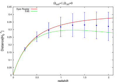
Figure 20: Average distance and distance dispersion at each redshift in the clumpy universe. The global universe is given by the EdS universe.

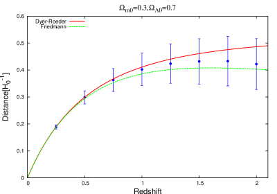
Figure 21: Same as in Fig. 20, but here the global geometry is given by the FL universe with $\Omega_{\Lambda 0}=0.7,\Omega_{\rm m0}=0.3$.

The distance dispersion given in our results is larger than the typical value of observational uncertainties evaluated without lensing effects (Crowder & Cornish, 2005). However, our evaluation presented in this section is very basic one. In order to apply this evaluation to the future observational data, we need more detailed information about other experimental uncertainties and degeneracies between the situation presented here and others. We leave this for future works.

6 Conclusion and summary

We have studied the distance-redshift relation obtainable through gravitational waves in a clumpy universe. We have assumed that all of the matter takes the form of uniformly distributed point masses with identical mass, $M_{L}$, and that the global geometry is described by the FL universe model. The distance from the source to the observer in the clumpy universe differs from that in the global universe, even if the redshift of the source is identical, since gravitational waves are magnified or demagnified by the gravitational lensing effect. We have numerically calculated the magnification due to multiple lensing effects in two extreme cases. In the first case, the wavelength $\lambda$ of the gravitational waves is much longer than the Schwarzschild radius, $2M_{L}$, of the point-mass lens. In the second case, the wavelength $\lambda$ is much shorter than $2M_{L}$.

In the case of long wavelengths, $\lambda\gg M_{L}$, the magnification due to a single lens is always very small, but it is not negligible. The total magnification in the multiple lens system is determined by the accumulation of all of the magnification effects due to each lens system, and is not small. We found that the relation between the average distance and redshift depends on the ratio $\lambda/M_{L}$, and it approaches the distance-redshift relation of the global universe as $\lambda/M_{L}$ increases. Furthermore, we found that the distance dispersion also depends on the ratio $\lambda/M_{L}$, and it approaches zero as $\lambda/M_{L}$ increases. The distance-redshift relation in the global universe is found even in the clumpy universe if the wavelength of gravitational waves is much longer than the Schwarzschild radius of the lens objects.

In the case of short wavelengths, $\lambda\ll M_{L}$, the geometrical optics approximation is valid. In order to calculate the total magnification, we employed the multiple lens plane method. We found that the distance dispersion is larger than that in the case of long wavelength. The total magnification comes from the focusing and interference effects on the ray bundles which emanate from the source to the observer. In this case, diffraction effects are negligible and thus the large magnifications due to the focusing effects on the ray bundles are possible. Moreover, interference effects can either enhance the magnifications or cause demagnifications.

These lensing effects cause a distance dispersion in the distance-redshift relations obtained from gravitational wave data, and we have shown its properties. In particular, we have clarified the dependence of the distance dispersion on the wavelength and the mass of the lens object. Making use of the properties of this distance dispersion, we can probe the inhomogeneities of our universe. The distance dispersion is sensitive to the ratio $M_{L}/\lambda$, and therefore our result suggest that we might use it to gain information about the typical masses of clumps that cause gravitational lensing effects. In order to obtain detailed information about the typical masses of lens objects, we need a method to calculate the case of $M_{L}\sim\lambda$ (Yamamoto, 2003).

Suppose that we observe gravitational waves from binaries of compact objects in a narrow wave band centered at $\lambda$. If the large distance dispersion does not appear in the distance-redshift relation obtained by these gravitational waves, we can impose a restriction on the typical mass scale of the clumping matters of $M_{L}\ll\lambda$. On the other hand, if a large distance dispersion appears, we can say that the mass of clumps $M_{L}$ is much larger than the wavelength of the gravitational waves.

In order to obtain a statistically reliable dispersion, we must detect a large number of gravitational waves. DECIGO’s planned sensitivity is $2\times 10^{-24}\rm{Hz}^{-1/2}$ around $1\rm{Hz}$; this means that $10^{5}$ chirp signals of coalescing binary neutron stars should be detected in 1 year (Seto et al., 2001). Therefore, it should be possible to obtain reliable distance dispersion measurements. For example, if we observe gravitational waves from binary neutron stars in the waveband centered at $1\rm{Hz}$, we can determine whether the typical mass scale $M_{L}$ of the dark matter that takes the form of macroscopic compact objects is much smaller or much larger than $10^{5}M_{\odot}$.

References

- Afonso et al. (2003) Afonso, C. et al. 2003 A&A, 400, 951
- Alcock et al. (2000) Alcock, C. et al. 2000 ApJ, 542, 281
- Claudel (2000) Claudel, C. M. 2000 Proc. Roy. Soc. Lond. A, 456, 1455
- Crowder & Cornish (2005) Crowder, J. and Cornish, N. J. 2005 Phys. Rev. D, 72, 083005
- Dyer & Roeder (1973) Dyer, C. C. and Roeder, R. C. 1973 ApJ, 180, 31
- Ellis et al. (1998) Ellis, G. F. R. , Bassett, B. A. and Dunsby, P. K. S. 1998 Class. Quant. Grav., 15, 2345
- Hawking & Israel (1989) Hawking, S. W. and Israel, W. 1989 300 Years of Gravitation (Cambridge University Press)
- Holz & Wald (1998) Holz, D. E. and Wald, R. M. 1998 Phys. Rev. D, 58, 063501
- Holz & Hughes (2005) Holz, D. E. and Hughes, S. A. 2005 ApJ, 629, 15
- Holz & Linder (2005) Holz, D. E. and Linder, E. V. 2005 ApJ, 631, 678
- Kantowski (1969) Kantowski, R. 1969 ApJ155, 89
- Kantowski (1998) Kantowski, R. 1998 ApJ, 507, 483
- Kibble & Lieu (2005) Kibble, T. W. B. and Lieu, R. 2005 ApJ, 632, 718
- Kocsis et al. (2006) Kocsis, B., Frei, Z., Haiman, Z. and Menou, K. 2006 ApJ, 637, 27
- Landau & Lifshitz (1962) Landau, L. D. and E. M. Lifshitz, E. M. 1962 The Classical Theory of Fields (Pergamon Press, Oxford)
- Linder (1988) Linder, E. V. 1988 A&A, 206, 190
- Markovic (1993) Markovic, D. 1993 Phys. Rev. D, 48, 4738
- Nakamura (1998) Nakamura, T. T. 1998 Phys. Rev. Lett., 80, 1138
- Nakamura & Deguchi (1999) Nakamura, T. T. and Deguchi, S. 1999 Prog. Theor. Phys. Suppl., 133, 137
- Nemiroff et al. (2001) Nemiroff, R. J., Marani, G. F., Norris, J. P. and Bonnell, J. T. 2001 Phys. Rev. Lett., 86, 580
- Paczyński (1986) Paczyński, B. 1986 ApJ, 304, 1
- Peters (1974) Peters, P. C. 1974 Phys. Rev. D, 9, 2207
- Peters (1964) Peters, P. C. 1964 Phys. Rev., 136, B1224
- Peters & Mathews (1963) Peters, P. C. and Mathews, J. 1963 Phys. Rev., 131, 435
- Rauch (1991) Rauch, K. P 1991 ApJ, 374, 83
- Rose (2001) Rose, H. G. 2001 ApJ, 560, L15
- Schneider et al. (1992) Schneider, P., Elers, J. and Falco, E. E. 1992 Gravitational Lenses (New York : Springer)
- Schutz (1986) Schutz, B. F. 1986 Nature, 323, 310
- Sereno et al. (2001) Sereno, M., Covone, G., Piedipalumbo, E. and de Riris, R. 2001 MNRAS, 327, 517
- Seitz & Schneider (1994) Seitz, S. and Schneider, P. 1994 A&A, 287, 349
- Seitz et al. (1994) Seitz, S., Schneider, P. and Ehlers J. 1994 Class. Quant. Grav., 11, 2345
- Seto et al. (2001) Seto, N., Kawamura, S. and Nakamura, T. 2001, Phys. Rev. Lett., 87, 221103
- Takahashi & Nakamura (2003) Takahashi, R. and Nakamura, T. 2003 ApJ, 595, 1039
- Takahashi (2006) Takahashi, R. 2006 ApJ, 644, 80
- Weinberg (1976) Weinberg, S. 1976 ApJ, 208, L1
- Wilkinson et al. (2001) Wilkinson, P. N., et al. 2001 Phys. Rev. Lett., 86, 584
- Yamamoto (2003) Yamamoto, K. 2003 arXiv:astro-ph/0309696.