Resolving Stellar Atmospheres I: The $\rm{H}\alpha$ line and comparisons to microlensing observations

Abstract

Context. We present work on $\rm{H}\alpha$ spectral line characteristics in PHOENIX stellar model atmospheres and their comparison to microlensing observations.

Aims. We examine in detail the $\rm{H}\alpha$ equivalent width (EW) and the line shape characteristics for effective temperatures of $4500$K$<T_{\rm{eff}}<5600$K where $\rm{H}\alpha$ is a strong spectral feature.

Methods. We find that $\rm{H}\alpha$ EW in models calculated under the assumption of local thermodynamic equilibrium (LTE) is up to 15% smaller than in models without this assumption, non-LTE models (NLTE) and that line shapes vary significantly for the two model types. A comparison with available high quality microlensing data, capable of tracing $\rm{H}\alpha$ absorption across the face of one G5III giant, shows that the LTE model that fits the EW best is about 100K hotter than and the best-fitting NLTE model has a similar $T_{\rm{eff}}$ as predicted by the spectral type analysis of the observed star but agree within the uncertainties of the observationally derived temperature.

Results. Neither LTE nor NLTE models fit the line shape well. We suspect unmodelled chromospheric emission. Line shape diagnostics suggest lower gravities than derived for the star and are unacceptable low in the case of the LTE models. We show that EW alone is insufficient for comparison to stellar model atmospheres, but combined with a new shape parameter we define is promising. In stellar parameter ranges where the $\rm{H}\alpha$ line is strong, a NLTE approach of modeling stellar atmospheres is not only beneficial but mandatory.

Conclusions.

1 Introduction

Most of our basic knowledge about the interior physics of stars, even of the Sun, is based on our understanding of stellar atmospheres. The modeling of such atmospheres allows us to derive the star’s fundamental characteristics such as temperature, gravity, chemical composition and age. However many outstanding questions still need to be answered about stellar atmospheres. The “solar model problem,” , i.e., the disagreement between model predictions for the neon-oxygen abundance ratio and measurements by helioseismology, is hotly debated (Drake & Testa, 2005; Asplund et al., 2003). Derivation of elemental abundances is based on the accuracy of stellar model atmospheres and as such make and shake our knowledge not only about stellar, but also about galactic and cosmic evolution (Asplund, 2003).

The main difficulty in constraining stellar atmosphere models with observations is that most techniques only measure the disk-integrated flux or disk-integrated spectra of stars. The biggest advance in one-dimensional (1-D) atmospheres modeling has been to introduce consistent treatment of Non-Local Thermodynamic Equilibrium (NLTE) processes (Anderson, 1989; Hauschildt & Baron, 1999). However observational tests of NLTE effects have been difficult to establish, because studying atmospheres of stars more distant than our Sun has proven difficult and tedious.

Various methods have been tried to resolve stars, i.e. measuring their sizes and resolving surface structure. Direct observations have been restricted to the Sun (e.g. Blackwell, Lynas-Gray, & Smith, 1995) or, when using the Hubble Space Telescope (HST), to nearby supergiants (e.g. Gilliland & Dupree, 1996). Doppler imaging (e.g. Oláh, Jurcsik, & Strassmeier, 2003) produces observed center-to-limb variations of the integrated flux that are in good agreement with values derived from current LTE model atmospheres. Whereas Interferometry (e.g. Aufdenberg et al., 2005) show less limb darkening than predicted by stellar atmospheres models. Due to the uneven surface of the moon, surface measurements of nearby giants via lunar occultations (Richichi & Lisi, 1990) have not yet yielded sufficient precision to distinguish between various model atmospheres. O’Donoghue et al. (2003) and Popper & Guinan (1998) have used eclipsing binaries to study surface structure. In such systems both stars are often in a similar evolutionary state, which complicates tremendously the decomposition of the single star spectra. Furthermore, if one star is evolved and has (almost) filled its Roche Lobe so that mass transfer occurs, then neither star is a good probe for single-star atmospheres. However all of these methods are restricted to nearby stars.

Microlensing was proposed to offer an elegant solution to the problem of observing distant stellar atmospheres (Schneider, Ehlers, & Falco, 1992). During a microlensing event a differential magnification pattern across the face of the source star enables the observer to resolve its surface (see §5 for more detail). Several authors have studied the effect theoretically. Heyrovský & Sasselov (2000) studied how microlensing can be used to detect stellar spots on the surfaces of stars. Heyrovský, Sasselov, & Loeb (2000) demonstrated the effects of microlensing on synthesized optical spectra of red giant model atmospheres. Heyrovský (2003) discussed the difficulty of microlensing light curve inversion methods. Bryce, Hendry, & Valls-Gabaud (2002) and Hendry, Bryce, & Valls-Gabaud (2002) examined the detectability of star spots via microlensing and their possible effects on multicolor microlensing light curves. Bryce, Ignace, & Hendry (2003) examined the change in line profiles due to bulk motion in circumstellar envelopes during microlensing fold caustic crossing events.

An early attempt by Lennon et al. (1996, 1997) used the magnification effect of the microlensing event 96-BLG-3 for spectral studies of stellar atmospheres. They further suggested an effect of center to limb variations on the $\rm{H}\alpha$ line profile during such an event. A number of well-studied microlensing events have resulted in measurements that resolve the source star; we discuss one of these in more detail in §5.1. The names and major characteristics of these events are listed in Table 1, with the respective publications. The major findings were promising comparisons of observationally-deduced limb darkening coefficients with model atmospheres and variations of equivalent width (EW) of the H$\alpha$ line. One of these events, EROS BLG-2000-5, is a cusp-crossing event, which shows that despite the increased complexity in modeling not only fold caustic crossings can be used for these purposes. For the most recent event, OGLE-2002-BUL-69 (Cassan et al., 2004; Kubas et al., 2005), a well-sampled light curve and high resolution spectra are available at crucial times during the event, making it a good target with which to compare high resolution model atmospheres. Four events of similar quality have been observed in 2004 and another four in 2005 and many more are to be expected in the years to come, making microlensing a viable future for testing stellar model atmospheres.

Event Name	Publication	results
MACHO Alert 95-30	Alcock et al. (1997)	$\rm{H}\alpha$ EW
MACHO 97-BLG-28	Albrow et al. (1999a)	limb darkening
MACHO 97-BLG-41	Albrow et al. (2000)	limb darkening
OGLE-1999-BUL-23	Albrow et al. (2001a)	limb darkening
MACHO 98-SMC-1	Albrow et al. (1999b)	limb darkening
EROS BLG-2000-5	Albrow et al. (2001b)	limb darkening
	Castro et al. (2001)	$\rm{H}\alpha$ EW
	Fields et al. (2003)
MOA 2002 -BLG-23	Abe et al. (2003)	limb darkening
OGLE-2002-BUL-069	Cassan et al. (2004)	$\rm{H}\alpha$ EW

Table 1: Observed microlensing events with characteristics and results. In the first column are listed microlensing events discussed in greater detail by the authors in the second column. The last column lists the main findings for the events, i.e. H$\alpha$ equivalent width variations and limb darkening coefficients were measured in the respective events.

This is the first in series of papers aimed at developing methods to test stellar atmosphere models by confronting them with observations that resolve stellar surfaces photometrically or spectroscopically. Based on the most current theoretical models, we describe what observations can be made in the future in order to distinguish between various stellar models and learn the most from comparisons to observations.

We lead into this work by describing, in §2, our methods and the PHOENIX stellar models. In §3 we explain the reasons for and analysis techniques of studying the $\rm{H}\alpha$ line. In §4, we introduce the spectral parameter range studied and show that spectral differences between LTE and NLTE cannot be ignored within the $\rm{H}\alpha$ line for stars with $4500K<T_{\rm{eff}}<5600K$. How microlensing can be used as a tool to resolve the surfaces of stars is described in §5, where we also present results of our comparison of model atmospheric data to microlensing $\rm{H}\alpha$ EW line data for the event OGLE-BULGE-2002-069.

In §6, we illustrate how to most appropriately choose the best-fitting model out of a set of models for a given parameter or set of parameters. In §7, we introduce a new line shape diagnostic and repeat the analysis similar to the EW analysis. Our conclusions are summarized in §8.

2 Methodology

2.1 Stellar Models

We study the state-of-art atmospheric models produced by the multi-purpose code PHOENIX (Hauschildt et al., 1999; Hauschildt, Allard, & Baron, 1999). These models are static and assume one-dimensional, spherically-symmetric radiative transfer. We have chosen PHOENIX because its models can be calculated for all stellar parameters from dwarfs to giants, for both static and variable stars. A major advantage of PHOENIX models is that the code can include self-consistently NLTE effects. LTE assumes that, within a confined region, absorption and emission of photons occurs at the same rate and the underlying region’s temperature structure follows a black body. NLTE models relax this assumption so that atomic physics may produce situations in which local areas need not be in thermal equilibrium. Spectra calculated from the PHOENIX models can be calculated for almost any resolution ranging from the UV to radio wavelengths.

In order to compare stellar model atmospheres to the observations of real stars we must “transform” the models into observables by simulating the effects of external phenomena on the spectra. Microlensing, for example see §5, would be such a transformation, as it occurs externally to the source star, but does affect the light collected by the observer as a function of time. Convolving model data with this transformation produces synthetic data, which we can then analyze in the same way as we would analyze observational data. We conduct a comparison between PHOENIX LTE and NLTE synthetic spectra as well as a comparison to high resolution observational spectral data from a microlensing event.

3 H$\alpha$ and its Equivalent Width

In this work we focus on the effects that can be studied with observations of the $\rm{H}\alpha$ line. The $\rm{H}\alpha$ line is a strong line for stars with $4500<T_{\rm{eff}}<5600K$ and is therefore a frequent observational target. Different parts of the $\rm{H}\alpha$ line are formed in different regions of a stellar atmosphere, some which are more affected by NLTE than others (Gray, 1992). This makes $\rm{H}\alpha$ a good candidate to study possible differences between LTE and NLTE modeling by testing these differences against observations. Another incentive to study $\rm{H}\alpha$ is that published data are available for the resolved source star during some microlensing events (Albrow et al., 2001b; Cassan et al., 2004). In this section, we concentrate on the EW of the line as a figure of merit with which to compare LTE with NLTE effects, and models with observations. We adopt the usual definition of EW:

$$EW=\int_{line}1-\frac{F_{\rm{line}}(\lambda)}{F_{\rm{cont}}(\lambda)}d\lambda$$ (1)

where $F_{\rm{line}}$ is the radiant flux as a function of wavelength $\lambda$, and $F_{\rm{cont}}$ the value of the flux from the continuous spectrum outside the spectral line. The analytical potential of EW as a tool for studying atmospheric models depends on one’s ability to measure its value consistently for both model and observational spectra, which requires a careful choice of the continuum and the rejection of spectral blends. In order to reduce systematically-introduced effects to the analysis, we apply the same algorithm to all our model and observational data.

3.1 Extracting Equivalent Width from Model Spectra and Data

For both model and observational data, the EW is determined as follows. We first apply a standard vacuum-to-air conversion to all model data. We then remove blended spectral lines and from this set of model/data points we determine the continuum around the spectral line that we wish to analyze and normalize the spectra. Note that by “continuum,” we mean the “pseudo continuum” determined by fitting, as there is no way of determining the real continuum for spectral line observations. After smoothing the data, we obtain the EW by spline interpolation followed by direct integration.

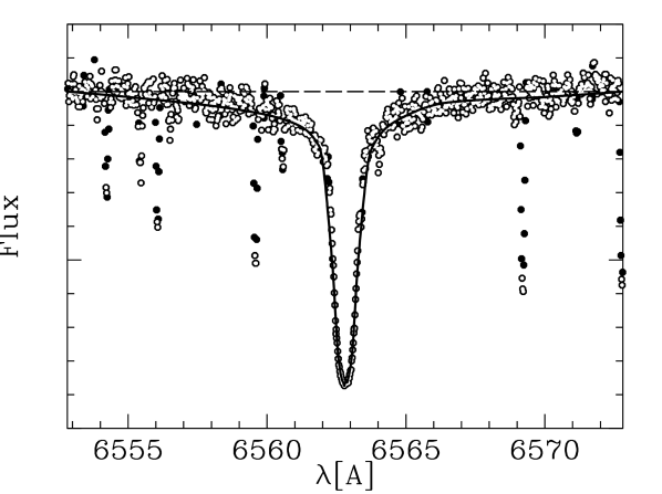
Figure 1: Illustration of our EW integration algorithm: black solid points are the model output data around the $\rm{H}\alpha$ line with added noise, distributed at random following a Gaussian with a root mean squared (rms) scatter $\sigma$ of $2.7\%$. Marked in white are those points chosen by the algorithm to be used for the integration. These are then binned, spline interpolated (black solid line), and integrated up to the continuum (long dashed line) to give the EW of the line.

Our clipping algorithm removes lines blended with $\rm{H}\alpha$ from the spectral data, which would otherwise contribute to the $\rm{H}\alpha$ EW during direct integration. We discard all points from the initial spectral data (whether model or fully-reduced observational data) that differ in flux from that of either of their neighbor points by more than a threshold, $\cal{T}$, which is determined by the signal-to-noise of the data and its spectral resolution, $\Delta\leavevmode\nobreak\ \lambda$ via,

$$\cal{T}=\rm{C}\sigma^{2}/\Delta\lambda\ ,$$ (2)

where $\sigma$ is the rms scatter of all flux points about their mean across the wavelength range considered. $C$ is a constant used to adjust the magnitude of the threshold to ensure optimal clipping. We chose $C$ by testing our clipping routine on different modeled and observed spectra, and found that a different value of C must be used within the core of the line in order to not reject spectral points corresponding to the line itself. After clipping, the continuum is then determined from the remaining points.

Figure 1 illustrates how we obtained the $\rm{H}\alpha$ EW in both synthetic and observed data. We assume the continuum to be linear over the narrow spectral range considered. We compute the mean flux value of the outermost 1$\AA$ of the spectra on either side of the $\rm{H}\alpha$ line, and fit a continuum line through these values. Although the synthetic data are virtually noiseless, we determine the continuum in this way so that the same method can be applied to the noisier observational data. We have tested and confirmed this method by determining the EW for integration ranges from 1$\AA$ to 10$\AA$. The slight increase in EW was linear from 9$\AA$ onwards, indicating that the line signature lies within $\pm$ 9$\AA$ and it is safe to determine the continuum outside of this range.

When smoothing, we divide the spectral data into three separate sections: (a) $6564.8\pm 1$$\AA$ to treat the core of the line, (b) the region excluding the core out to $6564.8\pm 3$$\AA$, to cover the wings, and (c) the transition to the continuum of the spectral range of $6564.8\pm 10$$\AA$, excluding the core and the wing regions. Within each of these spectral regions we adapt the sizes of bins over which we average so as to sample the continuum less densely than the wings, and the wings less densely than the core. The averaged flux values in each bin are then spline interpolated to give the EW of the line via direct integration.

4 The Stellar Parameter Grid: LTE vs NLTE

Using this algorithm, we obtained disk-integrated $\rm{H}\alpha$ EW values over a grid of 168 PHOENIX LTE and NLTE models. The stellar parameters ranged over a grid of $2.0<\log(g)<5.0$ in steps of $0.5$ and $4500K<T_{\rm{eff}}<5600K$ in steps of $100$K. A metalicity of [Fe/H]$=-0.5$ was assumed throughout.

Figure 2: Upper panel: contours of equal $\rm{H}\alpha$ EW (integrated over the face of the stellar disk) over a range of stellar parameters in $T_{\rm{eff}}$ and $\log(g)$ for LTE atmosphere models. Middle panel: Same, but for the NLTE atmospheric models. For the stellar parameter range shown, NLTE models have higher EW compared to LTE models at the same $T_{\rm{eff}}$ and $\log(g)$, as expected for the NLTE-affected $\rm{H}\alpha$ line. Lower panel: Contours of fractional difference $1-(EW_{\rm{LTE}}/EW_{\rm{NLTE}})$, given in percent.

In Figure 2, we indicate contour lines of equal $\rm{H}\alpha$ EW values. the results for both LTE and NLTE across the atmosphere model grid.

One can see immediately that $\rm{H}\alpha$ EW is very sensitive to changes in $T_{\rm{eff}}$, but much less so for changes in gravity. NLTE models with higher $T_{\rm{eff}}$ show a slightly stronger dependence on gravity than do the respective LTE models. Previous studies (e.g. Gray, 1992) have shown that NLTE calculations produce a deeper core for the $\rm{H}\alpha$ line than in the LTE regime, which we confirm. The bottom panel shows the fractional difference in $\rm{H}\alpha$ EW between the two model types.

Over the middle range of the grid, the fractional difference between LTE and NLTE is about 15%. This shows clearly that, within our stellar parameter grid, the difference between NLTE and LTE is significant, and that large systematic errors may compromise any conclusions drawn for the $\rm{H}\alpha$ line in this regime if LTE is assumed for its formation. This work also indicates that over the stellar range $T_{\rm{eff}}>5400K$ and $\log(g)<3.0$ a LTE approach may be reasonable for a study of the $\rm{H}\alpha$ line, depending on the precision required.

5 Microlensing as a Test: Resolving The Surface Of Stars

So far we have only compared models of stellar atmospheres. Can these differences be observed and, if so, how can this help us to understand better the underlying physics of line formation and stellar modeling? In particular, do we have ways to distinguish between NLTE and LTE effects at the limb and the center of stars? We might expect to observe larger differences at the limb, where less light originates from deeper layers of the star, as NLTE processes are more important in the outer, less dense regions of the atmosphere. Resolving the stellar surface then becomes crucial. A fairly new tool of resolving the surface of stars farther away than the Sun is microlensing (Bryce, Hendry, & Valls-Gabaud, 2002). When a stellar object, the lens, crosses the line of sight to a source star and the lens is a binary, an asymmetric magnification pattern, which peaks at the so-called caustic, moves across the face of a source star (see Figure 3). During such a caustic crossing there is a strongly differential magnification across the face of the microlensed star, which allows its surface to be resolved.

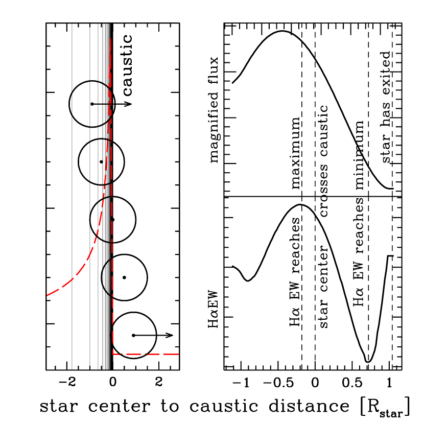
Figure 3: The effect of a microlensing caustic crossing on the integrated light and EW of the $\rm{H}\alpha$ line.: Left panel: As a star crosses a caustic, it becomes differentially magnified due to the asymmetric magnification pattern (red long dashes). Only the exit is shown. The vertical thin lines show contours of equal magnification leading up to the fold caustic line. Magnification drops immediately outside the caustic. Right panels show synthetic data for which a stellar model atmosphere has been convolved with a microlensing magnification pattern. The top panel shows how the total flux received from the star changes due to the magnification of the caustic. The bottom panel shows the respective changes in Halpha EW for this model. Note the weaker/stronger dips in EW that occur when the leading/trailing limb crosses the caustic, contributing emission (negative EW) to integrated light.

Figure 3 illustrates the microlensing effect on the total integrated light of the star (upper right panel) and on the $\rm{H}\alpha$ EW (lower right panel) during a caustic exit. Light from the parts of the star directly coincide with the position of the caustic are most highly magnified, and thus contribute a larger fraction to the integrated light observed.

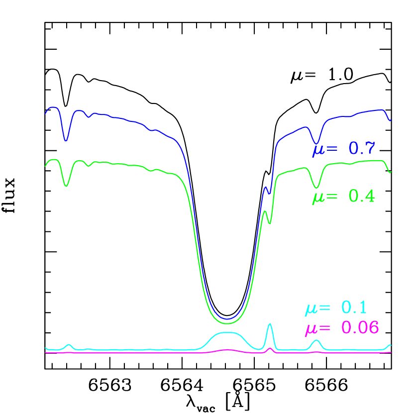
Figure 4: $\rm{H}\alpha$ spectral lines from stellar model atmospheres for different values of $\mu=\cos\theta$, where $\theta$ is opening angle to the line-of-sight. At the limb $\mu=0$ and $\mu=1$ in the center of the stellar disk. $\rm{H}\alpha$ is a strong absorption feature for most of the stellar disk, but near the limb $\rm{H}\alpha$ goes into emission.

Figure 4 illustrates the different shapes of the $\rm{H}\alpha$ spectral line across the face of the star for different values of $\mu=\cos\theta$, where $\theta$ is opening angle to the line-of-sight. $\rm{H}\alpha$ is a strong absorption line in the center of the star ($\mu=1$) and goes into emission near the limb. This emission explains the dip in the $\rm{H}\alpha$ EW during the caustic crossing while the limb is highly magnified.

Due to the relative motion of source and lens, the magnification pattern moves across the source star and produces a light curve of integrated stellar light, with a typical shape for microlensing events. The magnification pattern may be rather complex, but in most cases one can make the assumption that the caustic crossing is a fold caustic crossing, ie., that the caustic has no curvature across the face of the star. For what follows, we further assume that the source star is spherically symmetric, and that the relative motion of source star and caustic is constant and rectilinear. For fold caustics, a five-parameter fit to the light curve data is sufficient to extract the magnification pattern of the event and thus infer the contribution each part of the source star makes to the integrated light. The five parameters describe the time and duration of the event, the maximum magnification, how long it takes to reach maximum magnification and the underlying linear magnification after the caustic crossing (Albrow et al., 1999b). Entry into a caustic is unpredictable, but caustic exits can often be predicted so that proper observations can be put into place. Outside the caustic, typically there is little or no significant differential magnification across the stellar disk and the spectrum is similar to that of the unmagnified star. During the exit, integrated light is substantially influenced by the highly magnified light from the limb, only where differential magnification is important.

5.1 Variations of the $\rm{H}\alpha$ line EW during a fold caustic crossing: A worked example

Because the $\rm{H}\alpha$ line is in emission at the limb, the integrated EW of the $\rm{H}\alpha$ line drops during a caustic exit compared to the non-differentially magnified case. This occurs first when the leading limb crosses the caustic and experiences maximum magnification. The effect is stronger when the trailing limb crosses the caustic, as now most of the stellar disk has crossed into the low magnification region outside of the caustic and contributes a smaller fraction to the total integrated light than when most of the star still lies in the caustic interior.

During the microlensing event microlensing event OGLE-BULGE-2002-069 the PLANET collaboration was able to obtain high resolution VLT UVES data during the caustic exit (Cassan et al., 2004), and the collaboration kindly provided us with the fully-reduced spectra around the $\rm{H}\alpha$ line.

We adopted the parameterization of the fold caustic exit of the event from Cassan et al. (2004). For each time at which a UVES spectrum was available we produced an equivalent synthetic microlensed spectrum for both LTE and NLTE PHOENIX model atmospheres, for each atmospheric model on our stellar parameter grid.

We measured the $\rm{H}\alpha$ EW of the synthetic microlensed data via the algorithm described in §3, and applied the same algorithm to the observational data. Due to the virtual non-existence of noise in the synthetic data, we adjusted some values of the fitting parameters for the observational data: the clipping parameter $C$ was increased, and we have added an extra $8\AA$ outwardly to the range over which we determine the continuum to achieve a higher stability in the continuum. Also, since the observed width of the line is not reproduced by the models, as we describe later, the “core region” was defined as $\rm{H}\alpha\leavevmode\nobreak\ \pm\leavevmode\nobreak\ 0.9$$\AA$ in the data instead of $\rm{H}\alpha\leavevmode\nobreak\ \pm\leavevmode\nobreak\ 0.75$$\AA$ in the models.

Figure 5: Changes in the $\rm{H}\alpha$ EW for OGLE-BULGE-2002-069 during the course of its caustic exit. The solid lines represent the synthetic data for LTE (upper panel) and NLTE models (lower panel) for $T_{\rm{eff}}=5000$K, $\log(g)=2.5$ and [Fe/H] = -0.5, taken from our model grid, closest to those published by Cassan et al. (2004). The filled circles show our derivation of $\rm{H}\alpha$ EW from the spectra taken by Cassan et al. (2004). We corrected the observations for the systematic uncertainties in the EW determination for LTE and NLTE models computed from Monte-Carlo simulations, and applied their statistical uncertainties as errorbars. We did this separately for the high and low S/N regions. The double-ringed datapoints show observations taken 36 days after caustic exit.

Figure 5 shows our results, where the $\rm{H}\alpha$ EW is plotted for each time at which observations have been taken. (The last two points were taken long after the caustic exit to ensure two baseline points not affected the differential magnification.) We plot the $\rm{H}\alpha$ EW measurements for only one set of stellar parameters, namely: $T_{\rm{eff}}=5000$K, $\log(g)=2.5$ and [Fe/H]$=-0.5$. These are the parameters from our grid of stellar models that are closest to the stellar parameters given by Cassan et al. (2004) $T_{\rm{eff}}=5000$K, $\log(g)=2.5$ and [Fe/H] $=-0.6$. The difference in metallicity of 0.1 dex is well within observational errors of the metallicity determination. Further, in previous tests, we did not detect any mesurable changes in $\rm{H}\alpha$ EW from models with [Fe/H] $=-0.5$ to models with solar metallicity, so we are confident in our assumption that there are no effects from the 0.1 dex difference in metallicity.

We quantify the uncertainty in our determination of the $\rm{H}\alpha$ EW, using a Monte-Carlo approach simulating 999 noisy spectra by adding random noise to the virtually noiseless synthetic data and rerunning the algorithm to determine the EW. The simulations have been restricted to a stellar model of $T_{\rm{eff}}=5000$K and $\log(g)=2.5$. We assume no variation of the fractional error distribution across the whole stellar parameter grid. The random noise we add follows a Gaussian distribution with an rms scatter $\sigma$ equivalent to a signal-to-noise (S/N) of 130 or 50, which Cassan et al. (2004) quote for their spectra at a resolution of $\lambda/\Delta\lambda=30000$. These values translate into a signal-to-noise per spectral data point, spaced at $0.0174\AA$, of $(S/N)_{\rm{PP}}=36.5$, or $2.7\%$ noise, at those times where the center of the star is most highly magnified. At the caustic exit and post-exit time we obtain a $(S/N)_{\rm{PP}}=14$, or 7% noise. When we add this noise to the model spectra at the appropriate times, the model and observed spectra indeed appear to have a similar noise level. Thereafter, we shall use high and low S/N or noise to refer to the 2.7% and 7% noise levels respectively.

From the 999 simulations per noise level and model type, we determined a histogram of $\Delta\rm{EW}=\rm{EW}_{\rm{model,noisy}}-\rm{EW}_{\rm{model,noise-less}}$from noisy to noise-less data, fitted a Gaussian to these. The fitting parameters are listed in Table 2.

Simulation	$\mu_{\Delta\rm{EW}}[\AA]$	$\sigma_{\rm{EW}}[\AA]$	$\sigma_{\rm{EW}}[\%]$
LTE (high S/N)	0.03379	0.0492	3.28
LTE (low S/N)	0.03175	0.1626	10.8
NLTE (high S/N)	$-0.0623$	0.0586	3.45
NLTE (low S/N)	$-0.0912$	0.1509	8.88

Table 2: Parameters of Gaussian fits to the Monte-Carlo simulation results for determining systematic and statistical errors. We have separately determined these for LTE and NLTE models at high and low noise levels Both models have the same stellar parameters. The systematic error, $\mu_{\Delta\rm{EW}}$ is the amount that must be subtracted, on average, from the EW determined from noisy “data” compared to that determined from noiseless models. The scatter in EW determination about its known mean is $\sigma_{\rm{EW}}$

The scatter in the observational EW points is similar to the $\sigma_{\rm{EW}}$ determined from the model spectra. Large scatter appears to be mainly a continuum fitting effect. We fit a continuum to the spectra normalized by Cassan et al. (2004) in the same way as we do it for the models. Since the observational data is noisy, the continuum is more uncertain compared to noiseless model data. Even slight differences in the choice of the continuum will result in a larger scatter of EW values. Since the data have already been normalized by Cassan et al. (2004), for the observations we fit a continuum line with a fixed slope of zero. Our measurement of the continuum is slightly lower than that chosen by Cassan et al. (2004), but is consistent with the way we pick the continuum for the models.

The EW of the data determined in this way is shown in Figure 5 as dots; in the same figure, model predictions are also indicated. The overall trend of the observational data is reproduced by the models, however the offsets between them is obvious.

The LTE models do not match the magnitude of the EW of the $\rm{H}\alpha$ line of OGLE-BULGE-2002-069 after the caustic exit (double-ringed data points), where no differential magnification occurs and also at times when the center of the source star crosses the caustic. This could indicate that either the stellar atmosphere models are insufficient and/or we have chosen the wrong stellar parameters from the grid.

6 Giving the models a fair chance

Before condemning the model atmospheres prematurely, we need to be sure that we have chosen models that best fit the $\rm{H}\alpha$ EW data within uncertainties in the determination of $T_{\rm{eff}}$ and $\log(g)$. We quantify the discrepancy between models and observations by defining $\chi^{2}$, the goodness-of-fit figure of merit.

$$\chi^{2}=\sum_{t_{\rm{obs}}}\left[EW_{\rm{obs}}(t_{\rm{obs}})-EW_{\rm{model}}(t_{\rm{obs}})\right]^{2}/(\sigma_{\rm{EW}}^{2}(t_{\rm{obs}})\ ,$$ (3)

summing over all points in time $t_{\rm{obs}}$ at which an observed spectrum has been taken. We assume that any systematic errors introduced by our fitting algorithm and statistical uncertainties in fitting model spectra are the same across the model grid. Thus, for $\sigma_{\rm{EW}}$ we use the values derived in §5.1, namely, around 10% and 3.5% for the high and low noise data, respectively.

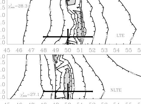
Figure 6: Upper panel: Contours of equal $\Delta\chi^{2}=\chi^{2}-\chi^{2}_{\rm{min}}$, where $\Delta\chi_{\rm{min}}^{2}$ is minimal when best agreement between LTE models and observations of the $\rm{H}\alpha$ EW of OGLE-BULGE-2002-069 are achieved. Lower panel: Same for NLTE. $\Delta\chi_{\rm{min}}^{2}$ is different for LTE and NLTE models and its value is shown in the left corner of the figure panels. The grey area indicates all models that lie within $3\sigma$ of the best fitting model for two degrees of freedom, namely $T_{\rm{eff}}$ and $\log(g)$. Further contour lines are the $4\sigma$, $5\sigma$ and higher boundaries. The tick marks on the contour lines indicate the direction of decrease in $\Delta\chi^{2}$. From their spectral analysis, Cassan et al. (2004) determined the stellar parameters to be $T_{\rm{eff}}=5000$K, $\log(g)=2.0$, [Fe/H]=-0.6. We mark this choice of parameters with the large cross with uncertainties of $\Delta T_{\rm{eff}}=\pm 200$K and $\log(g)=\pm 0.5$ as given in Minniti et al. (2002) for this type analysis.

We calculate $\chi^{2}$ for each model in our model stellar grid, and show in Figure 6, contours of equal $\Delta\chi^{2}$,

$$\Delta\chi^{2}=\chi^{2}-\chi^{2}_{\rm{min}}\ ,$$ (4)

where $\chi^{2}_{\rm{min}}$ is the minimal value of $\chi^{2}$ across the model grid, i.e. the goodness-of-fit for the best fitting model. Models along a contour line fit the observed measurements equally well. In Figure 6, we superimpose on the model grid the stellar parameters determined by Cassan et al. (2004) for OGLE-BULGE-2002-069. We follow an analysis of Minniti et al. (2002), used by Cassan et al. (2004), indicating uncertainties in determining stellar parameters of $\pm 200$K in $T_{\rm{eff}}$, $\pm 0.5$ in $\log(g)$, and $\pm 0.3$ in [Fe/H].

Within the uncertainties of the stellar model, LTE models with $\approx 100K$ higher $T_{\rm{eff}}$ than and NLTE models at the same values quoted by Cassan et al. (2004) provide the smallest $\chi^{2}$. Gravity is not well constrained. The overall goodness of fit is similarly poor for both LTE and NLTE models at a values of $\approx 28$ for 20 observations, which could be caused by random noise, with only about 7% confidence. Only the best fitting models should be examined to study further differences to the observations. Note that the best-fitting LTE and NLTE models have different temperatures.

7 The Importance of Line Shape

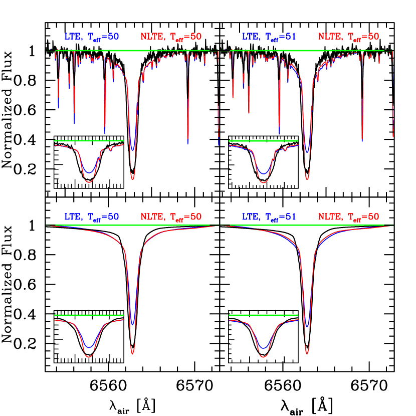
Figure 7: Differences in the spectra between observations of the $\rm{H}\alpha$ line for OGLE-BULGE-2002-069 (in black) and models (LTE in blue, NLTE in red) at the same magnification. The left panel shows comparison to the models with the stellar parameters closest to the published values, the right panel shows the spectra from models as chosen from Figure 6. Bottom panels present the clipped and spline interpolated lines after the observations and models have passed through the EW algorithm from §3.1. Each inset shows a narrower region around the core of the line. For all diagrams $\log(g)=2.5$ and $T_{\rm{eff}}$ is given per 100K.

Equivalent width collapses all the information about a spectral line into one value that only considers the area of the line under the continuum, but is independent of the line shape. This means that, despite a good agreement between the EW of a model spectral line, and of the observed spectral line any variations in the line shape will be ignored if this is the only figure of merit used to test models.

Examples of the $\rm{H}\alpha$ spectral line (top panel) and their fit from the algorithm (bottom) panel are shown in Figure 7 for one observation. The line from corresponding differentially magnified LTE and NLTE models with parameters as chosen from Cassan et al. (2004) are shown in the left panels, right panels give the best fitting stellar models as determined in Figure 6. Although the changes appear small, allowing stellar parameters $T_{\rm{eff}}$ and $\log(g)$ to vary within the observationally allowed uncertainties, can alter the EW by 10-15%, as can been seen in Figure 2.

That the models do not generally fit the width of the $\rm{H}\alpha$ line (see Figure 7) suggests that there are other physical processes occurring which are yet to be explained by stellar models. One explanation may be chromospheric influences, which Cassan et al. (2004) claim to have detected in their data. Since $\rm{H}\alpha$ is a chromospheric line but the standard model atmospheres do not include chromospheric calculations, more research is needed to explain this phenomenon.

This comparison of individual spectra clearly shows where discrepancies in EW occur, primarily in the wings of the line, but for LTE models also in the core of the line. However, the differences in shape in the core and the wings balance each other out when only total EW is considered. The discrepancies due to the different line shapes are washed out. Therefore we have devised a different diagnostic to compare model spectra with observational data by defining the line shape diagnostic, $\psi^{2}$,

$$\psi^{2}(t_{\rm{obs}})=\int_{\rm{line}}\left[{\cal{F}}_{\rm{obs,o}}(\lambda,t_{\rm{obs}})-{\cal{F}}_{\rm{model,o}}(\lambda,t_{\rm{obs}})\right]^{2}d\lambda\ ,$$ (5)

where we integrate the square of the flux difference that results when we subtract the model spectrum from the observational spectrum, after both have been normalized, clipped and spline-interpolated. Note, that the units of this new diagnostic are $\AA$, since the flux has already been normalized. Similarly, we can obtain ${\psi^{2}}$ for line shape comparisons between LTE and NLTE models.

Figure 8: Contours of equal ${\psi^{2}}$ for a NLTE-LTE model comparison. The tick marks on the contour lines indicate the direction of decrease. Measured by this quantity, line shapes for NLTE and LTE models differ least for lower $T_{\rm{eff}}$ and higher $\log(g)$ within the parameter grid. Larger differences are found for higher $T_{\rm{eff}}$ and higher $\log(g)$.

The result of which is shown in Figure 8 for non-microlensed model data. In order to compare LTE and NLTE models to observational data taken during a microlensing event, and to find the best-fit model based on the measured shape parameter, we define a new shape figure of merit

$$\Psi\equiv\sum_{t_{\rm{obs}}}{\psi^{2}}(t_{\rm{obs}})\,$$ (6)

which is sum of equally weighted ${\psi^{2}}$ over each observation during the event. The units of $\Psi$ are still $\AA$.

Defining the shape parameter $\Psi$ allows us to collapse the available time series data to one quantity per stellar model, while conserving the information of the line shape comparison. In effect, $\Psi$ is sum of $\chi^{2}$ comparison of all the spectra themselves, across a wavelength range defined by the line, equally weighted. We determine uncertainties in $\Psi$ by fitting a Gaussian to the distribution of $\Psi$ values resulting from 999 Monte-Carlo simulations. In each simulation we sum up 13 low noise and 7 high noise $\psi^{2}$ values randomly drawn from the distribution of $\psi^{2}$ values, which we have determined via 999 Monte-Carlo simulations in a similar fashion as for EW in §5.1 for low and high noise, LTE and NLTE models. We fit the resulting distributions of $\psi^{2}$ with a combination of a Gaussian and a straight line as the distribution is asymmetric because $\psi^{2}$ is positive definite. We fit the $\Psi$ distribution with a Gaussian convolved with a straight line. From this we deduce 3, 2 and 1$\sigma$ levels of confidence which we mark in Figure 9 as dark grey, light grey and the enclosed white areas.

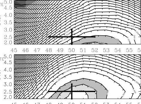
Figure 9: Contours of equal $\Psi-\Psi_{\rm{min}}$ for comparison of the observational data with LTE models (upper panel) and NLTE models (lower panel). The contours clearly constrain not only the $T_{\rm{eff}}$ but also the $\log(g)$ of the best fitting model parameters. This means that the best fitting LTE model has not only a higher $T_{\rm{eff}}$ and a lower $\log(g)$, whereas the best fitting NLTE model has stellar parameter closest to the one suggested by Cassan et al. (2004), indicated by the black cross.

In Figure 9, we show contour plots of equal $\Psi-\Psi_{\rm{min}}$, where $\Psi_{\rm{min}}$ is the lowest value of $\Psi$ across the model grid. For LTE models this is $\Psi_{\rm{min}}=0.71$, for NLTE models $\Psi_{\rm{min}}=0.47$. The shape parameter ${\psi^{2}}$ is much more dependent on $\log(g)$ than is EW, which was strongly dependent only on $T_{\rm{eff}}$. The dark grey shaded area indicates the 99.73% level of confidence around the best fitting model. The enclosed light grey and white areas show the 95.4% and 68.3% confidence levels, respectively. The best-fitting LTE model has a $\log(g)$ of less than 2.0, substantially less than what the observationally-determined stellar parameters suggest. As with fits to EW, LTE fits to the shape parameter, $\Psi$, again suggest a higher $T_{\rm{eff}}$ by about 200K, i.e. 100K higher than the EW-best-fitting LTE model suggested. Although the best-fitting NLTE model for the shape parameter leans towards lower gravities, these are in agreement with the observationally determined stellar parameters. The overall fit to $\Psi$, however, is fairly poor: The distribution of $\Psi$ at random shows that $99.9\%$ of values drawn randomly from the distribution of $\psi^{2}$ for NLTE models suggests a value below 0.07. For LTE models this reduces to a value less than 0.01.

8 Conclusions

As a part of a larger program to compare model atmospheres to observational data, we have developed an algorithm to consistently and automatically determine and compare spectral line characteristics. Here, we have focused on equivalent width (EW) of the $\rm{H}\alpha$ line and also introduced a line shape parameter $\psi^{2}$, which emphasizes flux differences between two spectra. We have studied a stellar parameter range of $4500<T_{\rm{eff}}<5300$ and $2.0<\log(g)<5.0$ at [Fe/H]$=-0.5$, a range typical of microlensed source stars in the Galactic Bulge.

We have determined the uncertainty of this algorithm by performing Monte-Carlo simulations in which noise is introduced to a model spectrum and the extraction procedure repeated. The simulations have been restricted to a stellar model of $T_{\rm{eff}}=5000$K and $\log(g)=2.5$. We assume no variation of the fractional error distribution across the whole stellar parameter grid. The EW of the $\rm{H}\alpha$ spectral line as predicted by PHOENIX atmospheric models is substantially different for LTE and NLTE model. The wrong choice of model type may result in uncertainties in EW larger than 8% for most models with $4500<T_{\rm{eff}}<5300$ and $2.0<\log(g)<5.0$. The shape parameter $\psi^{2}$ in an LTE-NLTE comparison is statistically significant and largest for high $T_{\rm{eff}}$ and high $\log(g)$.

Choosing the right model to compare to the observations is crucial when one wants to understand stellar atmosphere modeling. As an example, we study $\rm{H}\alpha$ spectral data from the microlensing event OGLE-BULGE-2002-069. First, we determine the best-fitting model to the $\rm{H}\alpha$ EW data over the range of our stellar grid for both LTE and NLTE models over the course of the caustic exit, during which the source star is resolved. We find that in order to fit the observed data an LTE model requires a $T_{\rm{eff}}$ about 100K larger than that proposed by Cassan et al. (2004) based on spectral type analysis for this source star. The best-fitting NLTE model, on the other hand, requires a $T_{\rm{eff}}$ as proposed by Cassan et al. (2004). The absolute $\chi^{2}$ is lower for NLTE PHOENIX models than for LTE models, suggesting a slight preference for the NLTE model.

Second, we determine the best-fitting model to the $\rm{H}\alpha$ $\psi^{2}$ which we define, and find that the best-fitting LTE model has a $T_{\rm{eff}}$, that is 200K higher than the observationally determined $T_{\rm{eff}}$ and a significantly lower $\log(g)$, The best-fitting NLTE model agrees with the observationally determined values for $T_{\rm{eff}}$ and $\log(g)$ within the uncertainties, although it tends to underestimate both $T_{\rm{eff}}$ and $\log(g)$ for this star. The NLTE models produced a better figure of merit than the LTE models for both diagnostics.

We caution, however, that declaring either LTE or NLTE models a failure based on analysis of $\rm{H}\alpha$ only is premature in the case of OGLE-BULGE-2002-069 . Chromospheric effects may alter the characteristics of the $\rm{H}\alpha$ line significantly, and the atmosphere models used here do not include chromospheres. Indeed, Cassan et al. (2004) claim to have detected an anomaly in the $\rm{H}\alpha$ line at some times during the caustic crossing that may be due to a chromosphere.

We would like to point out that with our method we are already placing strong constraints on $T_{\rm{eff}}$ and $\log(g)$ by using only two parameters measured for one particular line. Future studies of multiple lines and multiple diagnostics will provide even stronger constraints. In subsequent work, we will determine the most effective choices of spectral lines and their diagnostics for testing model atmospheres and include chromospheric calculations in the models for direct comparison to observations of OGLE-BULGE-2002-069.