Survey for Transiting Extrasolar Planets in Stellar Systems IV: Variables in the Field of NGC 1245

Abstract

The Survey for Transiting Extrasolar Planets in Stellar Systems (STEPSS) project is a search for planetary transits in open clusters. In this paper, we analyze the STEPSS observations of the open cluster NGC 1245 to determine the variable star content of the cluster. Out of 6787 stars observed with $V<22$, of which $\sim 870$ are cluster members, we find 14 stars with clear intrinsic variability that are potential cluster members, and 29 clear variables that are not cluster members. None of these variables have been previously identified. We present light curves, finding charts, and stellar/photometric data on these variable objects. Several of the interacting binaries have estimated distances consistent with the cluster distance determined from isochrone fits to the color magnitude diagram. Four stars at the main sequence turnoff of the cluster have light curves consistent with $\gamma$ Doradus variability. If these $\gamma$ Doradus candidates are confirmed, they represent the oldest and coolest members of this class of variable discovered to date.

1. INTRODUCTION

The dramatic increase in the number of surveys for planetary transits over the last five years has resulted in a wealth of high-precision stellar photometry (Horne, 2004). Although primarily conducted to detect planetary transits, such surveys also produce data sets that allow for intensive investigation of stellar variability. Especially useful are surveys of clusters, which can be used to characterize the variability content of the cluster. Detections of eclipsing binaries can provide a check on the cluster’s distance, as well as helping to characterize the mass-radius and mass-luminosity relationships.

Many surveys of clusters have already published data sets of high-precision photometry, finding low-amplitude variables, eclipsing binaries, and other pulsating stars. The PISCES (Planets in Stellar Clusters Extensive Search) project has observed clusters NGC 2158 and NGC 6791 (Mochejska et al., 2002, 2004, 2005). The EXPLORE/OC (Extrasolar Planet Occultation Research/Open Clusters) project has observed clusters NGC 2660 and NGC 6208 (von Braun et al., 2005). Other projects have observed or are observing NGC 7789, 6819, and 6940 (Street et al., 2003; Bramich et al., 2005), NGC 6633 (Hidas et al., 2005), and NGC 6705 (Hargis, Sandquist & Bradstreet, 2004).

The Survey for Transiting Extrasolar Planets in Stellar Systems (STEPSS) (Burke et al., 2002) concentrates on searching open clusters for planetary transits. Searching for transits in clusters is advantageous as clusters have known metallicities, ages, and stellar densities, and are therefore good laboratories for determining the distribution of planets without varying those stellar and environmental properties. Here we present an analysis of the observations of NGC 1245 to catalog the stellar variables in the cluster.

2. CLUSTER PARAMETERS AND OBSERVATIONS

See Burke et al. (2004) for a full discussion of the parameters of the cluster. NGC 1245 is a rich open cluster with an age of $1.04\pm 0.09$ Gyr. It has a metallicity slightly less than solar, [Fe/H] $=-0.05\pm 0.08$. The cluster is at a distance of $2.8\pm 0.2$ kpc, with distance modulus of $(m-M)_{0}=12.27\pm 0.12$. The core radius is $r_{c}=3.10\pm 0.52$ arcmin ($2.57\pm 0.43$ pc). The total cluster mass is $M=2700\pm 600M_{\odot}$. All errors given above are systematic, and are larger than the statistical errors.

The STEPSS project observed NGC 1245 over the course of 19 nights in October and November 2001. The observations were obtained with the MDM 8K mosaic imager on the MDM 2.4m Hiltner telescope yielding a $26\arcmin\times 26\arcmin$ field of view with $0.36\arcsec$ resolution per pixel. In total, the dataset consists of 936 $I$-band images with typical exposure times of 300 s. For the color magnitude diagram (CMD), several supplementary $B$ and $V$ band images were also obtained. None of the nights were photometric, and so a second series of observations was taken in February 2002 to calibrate the cluster photometry.

3. LIGHT CURVES AND STELLAR PROPERTIES

We follow the procedure outlined in Burke et al. (2005) to generate light curves, which develops a new method for differential photometry given the demands of detecting transiting extrasolar planets ($<0.01$ mag precision). The main features of the method include allowing each star to have a unique comparison ensemble, minimization of the light curve standard deviation as a figure of merit, and full automation. Applying this method yields light curves that have sub-1% precision for $V<18$.

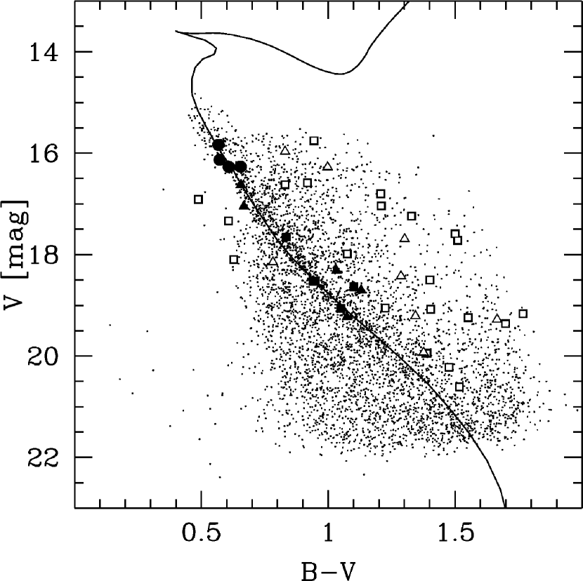
Of the 6787 stars identified in the survey’s field of view, we estimate $\sim 870$ belong to the cluster. This estimate comes from scaling and subtracting star counts from a control field on the outskirts of our field of view. Figure 1 shows the $V$, $\bv$ CMD of the cluster field along with the best-fit isochrone from Burke et al. (2004), derived from the theoretical isochrones of Yi et al. (2001). Given the cluster age, metallicity, distance, and reddening, the best-fit isochrone transforms an observed apparent magnitude into the stellar properties assuming the star is a cluster member. Using the stellar mass as the independent variable, we determine the stellar mass which minimizes the $\chi^{2}$ distance between the apparent magnitude and the best-fit isochrone magnitudes in the $BVI$ passbands.

Figure 1.— $V$, $\bv$ CMD for NGC 1245. Best-fit isochrone to the cluster main sequence (solid line). Filled shapes represent cluster variables, while open shapes represent field variables. The triangles show binary variables (see §5.1), the circles show $\gamma$ Doradus candidates (see §5.2), and the squares represent unclassified variables.

A caveat for assigning stellar properties based on the CMD is the assumption that the detected stellar light arises from a single main-sequence cluster member. The stellar properties contain significant systematic errors if the object does not belong to the cluster or if a portion of the stellar light arises from an unresolved stellar companion. The physical properties for the variable sources detected in this study should be regarded with extra caution considering that most sources of variability result from the binary nature of an object (Sterken & Jaschek, 1996) and thus have a large probability for significant stellar companion contamination.

4. VARIABLE STAR SELECTION

One of the great challenges in determining variability with high precision photometry is the difficulty of distinguishing intrinsic variability from noise and systematic errors. Common classes of variable stars demonstrate both large amplitude variations and periodic behavior, making them both easily detected and easily characterized. However, with the advent of surveys which observe thousands of stars with millimagnitude photometry, robustly detecting variations at low noise levels requires a variety of statistical selection criteria. Some surveys, such as ASAS, the All Sky Automated Survey (Eyer & Blake, 2005), and OGLE, the Optical Gravitational Lensing Experiment (Mizerski & Bejger, 2002), have developed automated classification pipelines. Many surveys, though, use a few simple statistical cuts to identify variable stars independent on the source or type of variability.

Our variability selection routine has three stages. First, we eliminate outlying measurements, and require a minimum number of remaining measurements. Second, we compute three different statistics that describe the behavior of the lightcurve: the root-mean-square (RMS), the Stetson $J$ statistic (Stetson, 1996), and the AoV periodicity statistic Schwarzenberg-Czerny (1996). We apply cuts on each of those values to select variable candidates. Third, we visually inspect the lightcurves and images of the variable candidates to eliminate false positive candidates with variability due to blending effects from nearby objects or detector defects. In §4.4, we describe two tiers of statistical cuts. The first, more stringent cut does not contain any false positives. A second, less stringent, cut with higher sensitivity contains lower amplitude variables, but also contains $<$ 7% false positives, which are later eliminated through visual inspection.

4.1. Eliminating Outlying Points

The first stage of the analysis removes statistically outlying photometric measurements. Outliers are identified in the following manner: For each star we calculate the reduced chi-square light curve variability,

$$\chi^{2}=\frac{1}{n-1}\sum_{k=1}^{n}\frac{(m_{k}-\mu)^{2}}{\sigma_{k}^{2}},$$ (1)

where the sum is over $n$ observations, $m_{k}$, with error $\sigma_{k}$, and $\mu$ is the weighted average magnitude of the light curve,

$$\mu=\frac{\sum_{k=1}^{n}m_{k}/\sigma_{k}^{2}}{\sum_{k=1}^{n}1/\sigma_{k}^{2}}\,.$$ (2)

The $\chi^{2}$ statistic measures the degree to which a constant light curve model approximates the light curve data within the context of the measurement errors. Light curves with intrinsic variability result in high $\chi^{2}$ values, denoting that a constant light curve model poorly represents the data. Before eliminating outlying measurements, we scale the errors by setting $\sigma_{k}^{{}^{\prime}2}=\sigma_{k}^{2}\chi^{2}$, thus enforcing $\chi^{2}=1$. The error scaling allows the Gaussian noise, systematic error, or intrinsic variability (whichever noise source dominates the scatter in the light curve) to set the scale for judging whether a measurement is a statistical outlier. This procedure can eliminate intrinsic variability that affects a small number of the measurements. This hampers our ability to detect large amplitude eclipsing binaries when only a single eclipse occurred during the observations. However, given our quantitative selection criteria and documented analysis techniques, these biases can easily be accounted for with a more detailed inspection of the data.

For each observation, we compute the deviation, $\delta_{k}=|m_{k}-\mu|/\sigma_{k}^{{}^{\prime}}$. All photometric measurements with $\delta_{k}>3$ are eliminated. We perform three iterations of the above procedure for each light curve. The light curves with $<$750 measurements remaining typically result from false stellar detections near the cores of bright isolated stars and are discarded. We also eliminate light curves with RMS $<0.3$ mag, since no light curves with higher scatter show any kind of coherent intrinsic variability.

4.2. The Stetson $J$ Statistic

The Stetson $J$ statistic (Stetson, 1996) provides our primary measure of the coherent intrinsic light curve variability. The statistic measures variability by weighting photometric variations that are correlated in time. A light curve with a steady change in brightness over a period of time results in a higher $J$ value than a curve with Gaussian noise, even though both curves may have equal values for $\chi^{2}$. The statistic is defined by

$$J=\frac{\sum_{k=1}^{n}w_{k}\,\,{\rm sgn}(P_{k})\sqrt{|P_{k}|}}{\sum_{k=1}^{n}w_{k}},$$ (3)

where the observer defines $n$ pairs of observations with weights $w_{k}$. We define observations as a pair when they are separated by less than 0.02 days. $P_{k}$ is the product of the normalized residuals of two observations $i$ and $j$, constituting the $k$th pair, such that

$$P_{k}=\left\{\begin{array}[]{ll}\delta_{i(k)}\delta_{j(k)},&\mbox{if $i(k)\neq j(k)$}\\ \delta_{i(k)}^{2}-1,&\mbox{if $i(k)=j(k)$}\end{array}\right.$$ (4)

and $\delta$ is the “relative error”, defined as

$$\delta=\sqrt{\frac{n}{n-1}}\frac{m-\mu}{\sigma},$$ (5)

where $m$ is the apparent magnitude of the star, $\sigma$ is the error in the magnitude, and $\mu$ is the weighted mean magnitude of the star. Following the choices of Kaluzny et al. (1998), we set $w_{k}=1$ for pairs of observations ( $i(k)\neq j(k)$ ) and $w_{k}=0.25$ for single observations ( $i(k)=j(k)$ ), and we also multiply the final quality $J$ by $\sum_{k=1}^{n}w_{k}/w_{max}$, where $w_{max}$ is the total weight the star would have if it were measured on all images.

Of the stars we observe, the Stetson statistic varies from $J\ll 1$ for nonvariable sources, to $1<J<10$ for obvious variables. For objects with $J\approx 1$, it can be difficult to demarcate a specific cut in $J$ to specify variability. We describe our choices for cuts on $J$ in §4.4.

4.3. Periodicity Analysis

To select periodic variations, we apply the Multiharmonic Analysis of Variances (ANOVA) period-search algorithm described by Schwarzenberg-Czerny (1996). Given a range of periods, the ANOVA algorithm produces a likelihood statistic, $0\leq AoV\leq 1$, that returns the quality of fit for orthonormal polynomials to the light curve variability. Since the observations occurred over a duration of 19 days, we run the ANOVA algorithm over a period range of 0.1 days to 14 days, which we believe to be the variability periods that we could reasonably detect.

One problem with applying the ANOVA algorithm to ground-based observations is the appearance of significant light curve variability on the diurnal period and its aliases. The rise and set of the field of observation and the corresponding secular changing atmospheric path length and mechanical stresses on the telescope impart systematic errors in the light curve. Our light curves display trends in the light curve variability as a function of seeing. In §3 we correct for these trends, but trends above the expected Gaussian noise remain. We find signs of aliasing primarily at periods of 1/3, 1/2, 2/3, 1, 2, 3, and 4 days. Relying on the ANOVA statistic alone results in many detections of low amplitude ($<$ 0.01 mag) variables with periods at the diurnal period and its aliases. However, in combination with the Stetson $J$ statistic (see §4.4) these alias variables do not make it into the final variable object samples.

4.4. Final Cuts and Visual Inspection

There are several systematic effects that complicate the attempt to impose categorical cuts in $J$ and $AoV$ that result in a sample that includes all probable intrinsic variables and zero false detections. Systematic errors in the light curve, such as blended objects, edge effects, detector defects, and detector saturation can artificially inflate $J$ and $AoV$ for non-variable sources. Furthermore, such effects, along with poor photometry, can in some cases lead to lower $J$ and $AoV$ values for true variables, compared to perfect photometry. We conclude that the most useful evaluation of the variability in our sample is a two-tier selection, in which we identify stars with robust variability and zero false detections, and then a second tier of candidate variables with a less stringent selection and resulting in sample with some low contamination due to false detections.

Our first tier consists of stringent cuts on the $J$ and $AoV$ statistical values. We find that cuts of $J>1.2$ and $AoV>0.65$ yield an ensemble of 23 stars which are all clearly intrinsic variables. The first tier has zero contamination due to false positives. However, it misses a number of other clear variables that vary with lower amplitudes. We then conduct a visual inspection of the images of the remaining sources, and flag those that are near detector defects such as bad columns, diffraction spikes, bleed trails, etc. A second tier cut of $J>0.75$ and $AoV>0.55$ includes most stars in our sample that have coherently varying light curves and includes few false positives. This second cut contains 44 variable candidates, including all the first tier objects. Visual inspection of the lightcurves and images of these stars enables us to eliminate three of the second tier stars due to detection effects, yielding a contamination rate of $\sim 7\%$. Based on a visual inspection of light curves, the contamination rate climbs rapidly for lower statistical cuts. Upon visual inspection of stars that do not make the cuts, we do find two more field stars that show coherent, periodic variability at low amplitudes. We include these two stars in our field star sample.

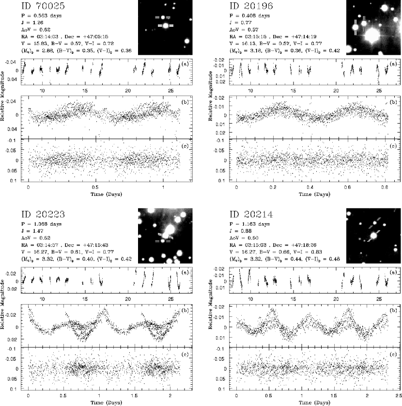
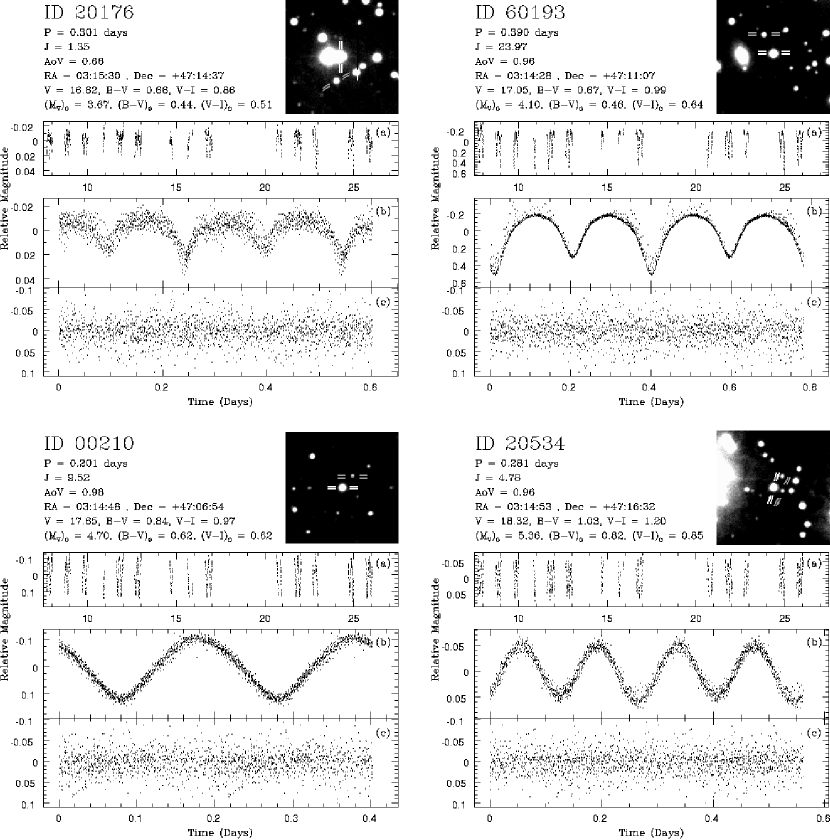
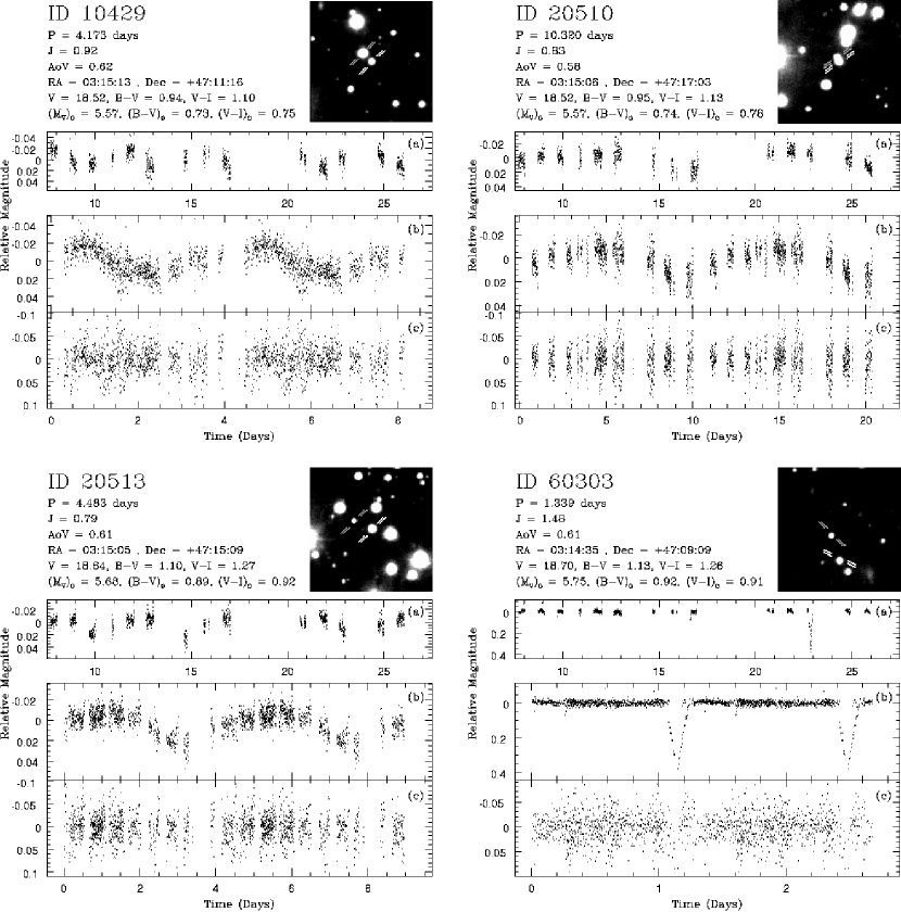
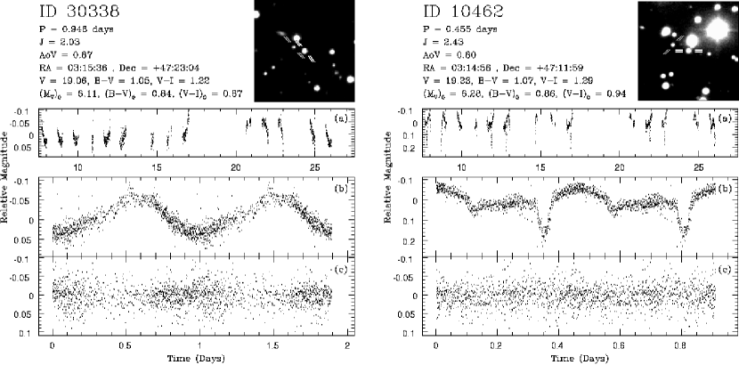
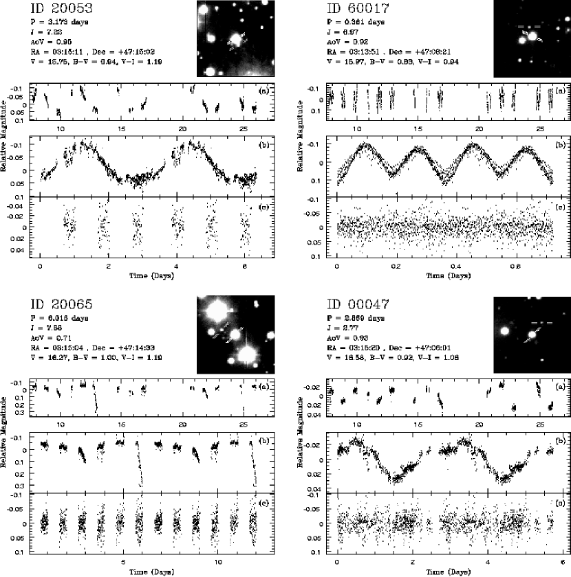
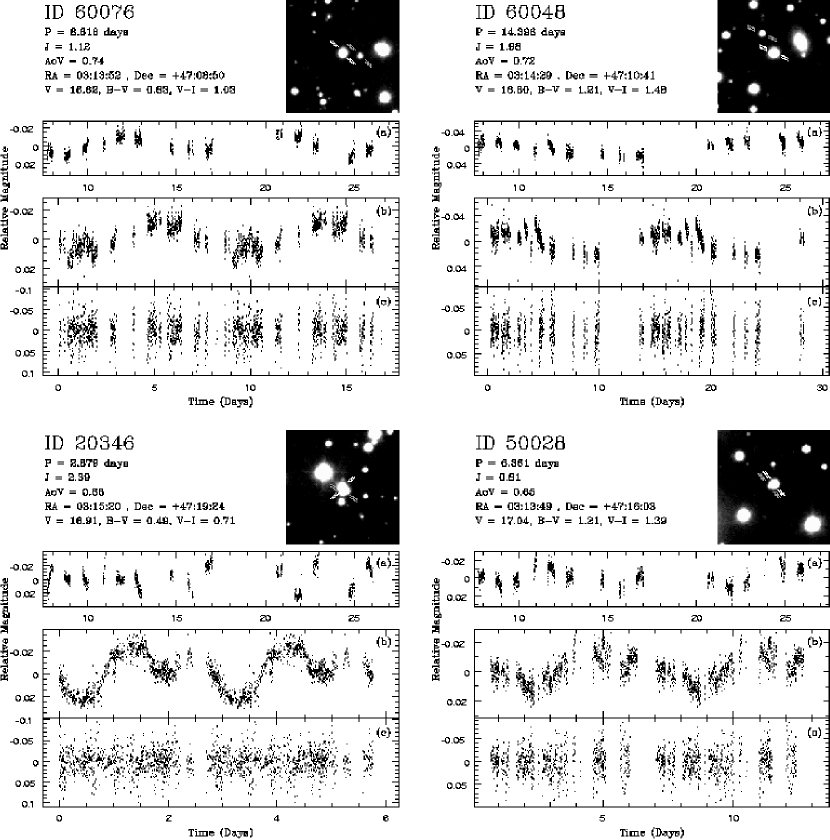
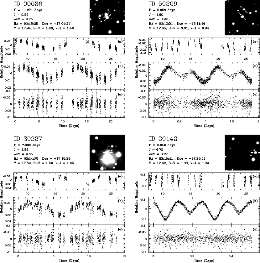
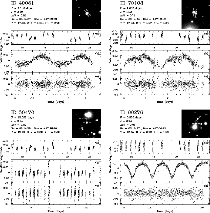
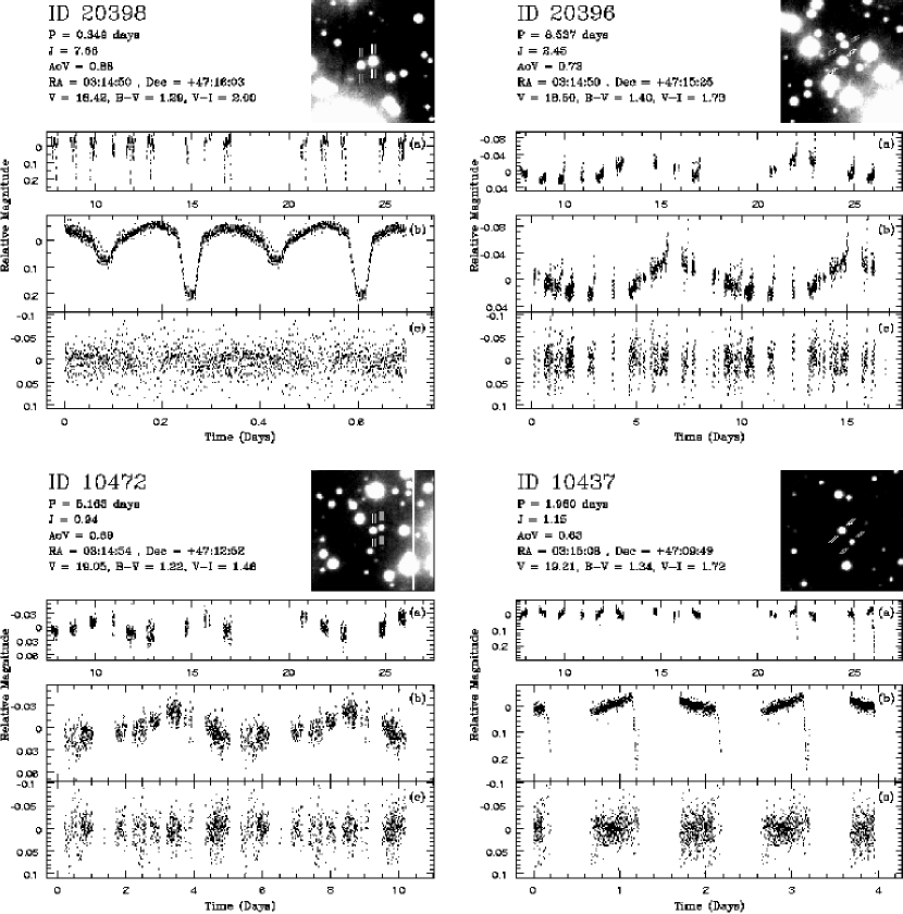
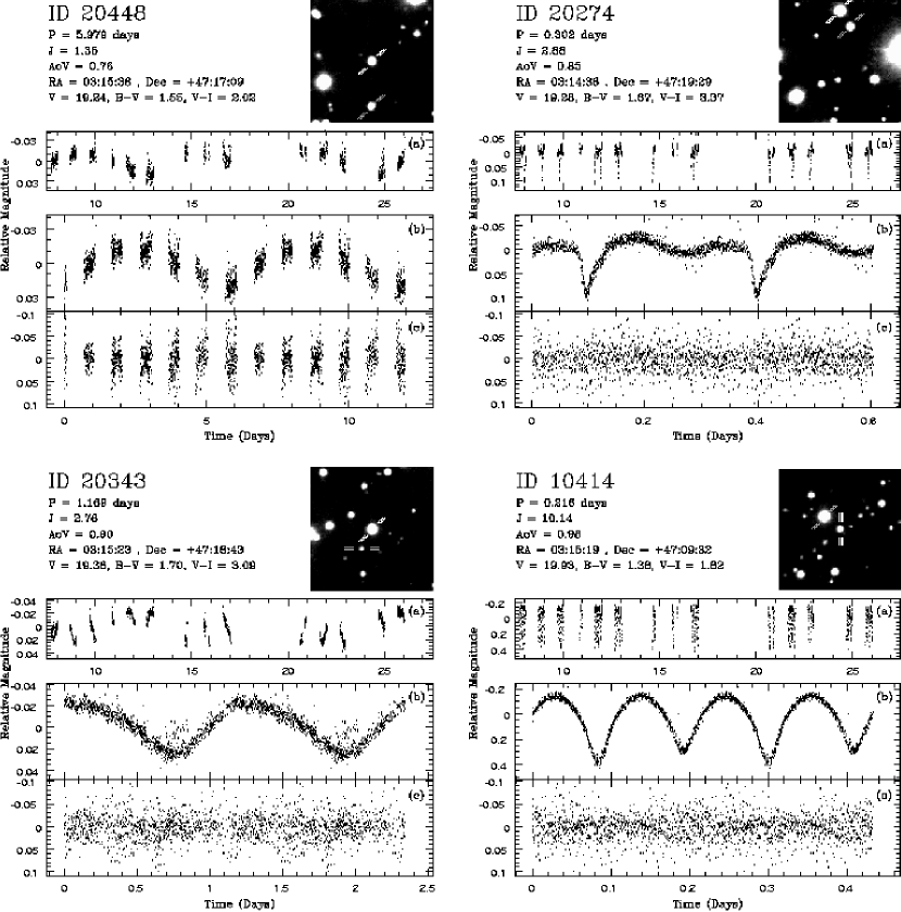
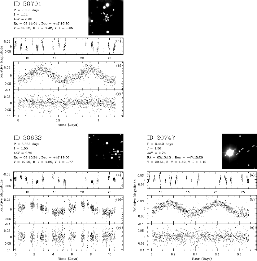
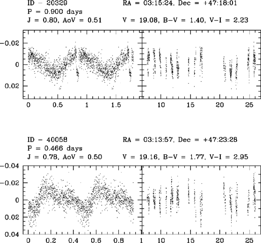
We show the light curves and photometric properties of the potential cluster members meeting both selection cuts in Figures 2 though 6. The plots for the field variables are in Figures 7 though 12. For each variable we show the unphased lightcurve in panel (a) for the full 19 days of the survey. In panel (b) we show the phased lightcurve of the variable, with two periods plotted. In the upper right corner is a finding chart showing the variable marked with white bars. The nearest detected object is marked with gray bars, and the light curve for the nearest object is shown in panel (c), phased to the period of the variable. We show the phased lightcurve for the nearest source because some of the millimagnitude amplitude variables are visually blended. Having an object nearby with similar blending complications that does not reveal variability confirms the intrinsic nature of the low amplitude variable. For completeness, we also show light curves in Figure 13 for two objects that do not survive the second tier cuts, but visually demonstrate intrinsic variability.

It should be noted that the DoPhot photometry detection software cannot successfully identify every object in the images. Objects that are too heavily blended, elongated, faint, saturated, etc., do not make it through the photometry pipeline. Therefore, the nearest object identified by the software may not be the nearest object to the variable. In most cases, however, the object identified as nearest is still close enough to the variable for the light curve comparison to be useful.

We plot the properties of the potential cluster variables in Table 1, and the field variables in Table 2, with the two visually selected stars listed separately. For a variable to belong to the cluster it must have $BVI$ apparent magnitudes consistent with the cluster main sequence. For potential cluster members, we give estimates for the stellar properties based on the CMD (see §3), and we classify their variable types (see §5) if possible. Both tables give magnitudes and positional data for all the variable stars.

Figure 2.— Light curves and finder charts for variables that are potential cluster members. In the top right is the finder chart, with the variable marked with the white bars and the nearest detected object marked with gray bars. Panel (a) shows the full unphased light curve for the variable. Panel (b) shows the variable’s light curve phased to the nearest period, with two periods plotted. Panel (c) shows the light curve of the nearest object phased to the period of the variable.

Figure 3.— Light curves and finder charts for potential cluster variables. See caption of Figure 2 for description.

Figure 4.— Light curves and finder charts for potential cluster variables. See caption of Figure 2 for description.

Figure 5.— Light curves and finder charts for potential cluster variables. See caption of Figure 2 for description.

Figure 6.— Light curves and finder charts for field star variables. See caption of Figure 2 for description.

Figure 7.— Light curves and finder charts for field star variables. See caption of Figure 2 for description.

Figure 8.— Light curves and finder charts for field star variables. See caption of Figure 2 for description.

Figure 9.— Light curves and finder charts for field star variables. See caption of Figure 2 for description.

Figure 10.— Light curves and finder charts for field star variables. See caption of Figure 2 for description.

Figure 11.— Light curves and finder charts for field star variables. See caption of Figure 2 for description.

Figure 12.— Light curves and finder charts for field star variables. See caption of Figure 2 for description. The brightness scaling for the finder chart for object 20747 is different from the other finder charts, with objects appearing dimmer, so that the bright star in the left of the chart does not swamp the variable. For that reason, the nearest identified star is not visible in this scaling.

Figure 13.— Light curves for two objects that did not survive the variability cuts, but show coherent periodic variability upon visual inspection. Phased lightcurves showing two full periods are shown on the left, and the full unphased light curves are shown on the right.

Table 1Properties of Variable Potential Cluster Members

STEPSS	$(M_{V})_{0}$	$(B-V)_{0}$	$(V-I)_{0}$	RA	Dec	Variable	$M$	$R$	($T_{eff}$)	$J$	$AoV$	Period
ID #				(2000.0)	(2000.0)	Type	($M_{\odot}$)	($R_{\odot}$)	(K)			(days)
70025	2.88	0.35	0.36	03 14 03	+47 05 15	$\gamma$ Dor	1.47	1.56	7000	1.262	0.619	0.563
20196	3.18	0.36	0.42	03 15 15	+47 14 19	$\gamma$ Dor	1.40	1.45	6800	0.774	0.566	0.408
20223	3.32	0.40	0.42	03 14 57	+47 15 43	$\gamma$ Dor	1.36	1.40	6700	1.470	0.619	1.068
20214	3.32	0.44	0.48	03 15 03	+47 18 26	$\gamma$ Dor	1.36	1.40	6700	0.877	0.604	1.163
20176	3.67	0.44	0.51	03 15 30	+47 14 37	EW	1.28	1.28	6500	1.352	0.656	0.301
60193	4.10	0.46	0.64	03 14 28	+47 11 07	EW	1.19	1.16	6300	23.966	0.962	0.390
00210	4.70	0.62	0.62	03 14 48	+47 06 54	–	1.07	0.98	5900	9.515	0.977	0.201
20534	5.36	0.82	0.85	03 14 53	+47 16 32	EW	0.96	0.85	5600	4.777	0.960	0.281
10429	5.57	0.73	0.75	03 15 13	+47 11 16	–	0.93	0.82	5400	0.921	0.623	4.173
20510	5.57	0.74	0.78	03 15 06	+47 17 03	–	0.93	0.82	5400	0.827	0.584	10.32
20513	5.69	0.89	0.92	03 15 05	+47 15 09	–	0.91	0.80	5400	0.794	0.611	4.483
60303	5.76	0.92	0.91	03 14 35	+47 09 09	EA	0.89	0.79	5300	1.478	0.609	1.339
30338	6.11	0.84	0.87	03 15 36	+47 23 04	–	0.85	0.75	5100	2.034	0.873	0.946
10462	6.28	0.86	0.94	03 14 56	+47 11 59	EA	0.83	0.73	5100	2.434	0.799	0.455

Table 2Properties of Variable Field Stars

STEPSS ID #	$V$	$B-V$	$V-I$	RA	Dec	$J$	$AoV$	Period
				(2000.0)	(2000.0)			(days)
20053	15.75	0.95	1.18	03 15 11	+47 15 02	7.223	0.945	3.173
60017	15.98	0.82	0.95	03 13 51	+47 08 21	6.974	0.924	0.361
20065	16.28	0.99	1.20	03 15 04	+47 14 33	7.879	0.707	6.016
00047	16.59	0.91	1.06	03 15 20	+47 06 01	2.770	0.931	2.869
60076	16.62	0.83	1.03	03 13 52	+47 08 50	1.118	0.736	8.618
60048	16.80	1.20	1.48	03 14 29	+47 10 41	1.979	0.721	14.40
20346	16.91	0.49	0.71	03 15 20	+47 19 24	2.387	0.876	2.879
50028	17.04	1.21	1.39	03 13 49	+47 16 03	0.808	0.652	6.361
00036	17.24	1.33	1.52	03 15 28	+47 04 27	0.856	0.784	11.27
50209	17.33	0.61	0.84	03 13 51	+47 14 26	1.901	0.916	0.936
20237	17.59	1.50	1.95	03 14 52	+47 19 25	1.887	0.846	7.306
30143	17.69	1.30	1.29	03 15 41	+47 26 01	6.753	0.974	0.252
40061	17.72	1.51	2.06	03 14 07	+47 22 03	2.191	0.868	1.130
70108	17.99	1.07	1.35	03 14 04	+47 03 22	1.019	0.711	1.822
50470	18.10	0.62	0.86	03 14 28	+47 16 36	0.843	0.666	12.03
00276	18.15	0.78	1.06	03 15 37	+47 04 45	8.737	0.953	0.304
20398	18.42	1.29	2.00	03 14 50	+47 16 03	7.660	0.885	0.349
20396	18.50	1.40	1.73	03 14 50	+47 15 25	2.449	0.731	8.537
10472	19.05	1.23	1.45	03 14 54	+47 12 52	0.939	0.688	5.163
10437	19.21	1.34	1.72	03 15 08	+47 09 49	1.145	0.633	1.980
20448	19.24	1.56	2.02	03 15 36	+47 17 09	1.349	0.764	5.979
20274	19.28	1.66	3.37	03 14 36	+47 19 29	2.880	0.854	0.302
20343	19.36	1.70	3.09	03 15 23	+47 18 43	2.758	0.899	1.169
10414	19.93	1.38	1.82	03 15 19	+47 09 32	10.143	0.980	0.216
20632	19.95	1.39	1.78	03 15 24	+47 19 56	1.051	0.700	5.365
50701	20.22	1.48	1.95	03 14 04	+47 16 20	1.111	0.682	0.606
20747	20.61	1.52	3.11	03 15 15	+47 15 29	1.056	0.756	0.442
20329	19.08	1.40	2.23	03 15 24	+47 18 01	0.796	0.511	0.900
40058	19.16	1.77	2.95	03 13 57	+47 23 28	0.782	0.503	0.931

4.5. Matching To 2MASS

Most of the selected variables have matching counterparts in the 2MASS database (Skrutskie et al., 1997), which we accessed through the VizieR web portal. For variables with a 2MASS counterpart within 1$\arcsec$ radius, we list the 2MASS ID numbers, the 2MASS magnitudes in the $J$, $H$, and $K$ bands, and the distance between the variable positions we measure and the reported positions of the 2MASS sources. Three of the faintest stars, two cluster members and one field star, were not matched to any 2MASS object. A search of the literature revealed no known variable counterpart to any of the variable stars identified in this analysis. We were unable to find any published cases of variable stars in the observed field within the magnitude ranges we searched. We therefore conclude that all of the variables identified in this paper are previously unknown.

Table 3Variable Matches to 2MASS

STEPSS ID	2MASS ID	2MASS Offset	$J$	$H$	$K$
		(arcsec)
Cluster Members
00210	03144786+4706544	0.098	16.116 $\pm$ 0.094	15.670 $\pm$ 0.120	15.881 $\pm$ 0.065
20534	03145325+4716321	0.579	16.270 $\pm$ 0.107	15.683 $\pm$ 0.124	15.512 $\pm$ 0.172
20176	03152956+4714374	0.066	15.240 $\pm$ 0.044	14.901 $\pm$ 0.059	14.677 $\pm$ 0.069
60193	03142811+4711067	0.079	15.757 $\pm$ 0.072	15.245 $\pm$ 0.091	15.348 $\pm$ 0.158
20196	03151490+4714185	0.043	14.904 $\pm$ 0.030	14.670 $\pm$ 0.051	14.555 $\pm$ 0.060
10429	03151250+4711157	0.232	16.635 $\pm$ 0.149	15.760 $\pm$ 0.068	14.873 $\pm$ 0.101
10462	—
70025	03140339+4705144	0.115	14.747 $\pm$ 0.040	14.509 $\pm$ 0.051	14.483 $\pm$ 0.069
30338	—
20223	03145747+4715430	0.063	14.922 $\pm$ 0.043	14.733 $\pm$ 0.065	14.531 $\pm$ 0.080
20214	03150277+4718258	0.063	14.939 $\pm$ 0.033	14.621 $\pm$ 0.048	14.598 $\pm$ 0.077
60303	03143504+4709095	0.363	16.608 $\pm$ 0.150	16.140 $\pm$ 0.180	15.785 $\pm$ 0.216
20513	03150464+4715090	0.356	16.438 $\pm$ 0.117	15.938 $\pm$ 0.153	16.060 $\pm$ 0.030
20510	03150636+4717030	0.572	16.396 $\pm$ 0.116	16.033 $\pm$ 0.168	15.821 $\pm$ 0.230
Field Stars
10414	03151946+4709324	0.483	17.050 $\pm$ 0.151	16.311 $\pm$ 0.173	16.243 $\pm$ 0.283
30143	03154104+4726009	0.109	15.495 $\pm$ 0.048	14.874 $\pm$ 0.064	14.804 $\pm$ 0.095
20274	03143588+4719290	0.056	14.097 $\pm$ 0.025	13.486 $\pm$ 0.027	13.140 $\pm$ 0.030
00276	03153653+4704457	0.483	16.386 $\pm$ 0.096	15.946 $\pm$ 0.156	15.708 $\pm$ 0.198
20398	03144954+4716030	0.124	15.156 $\pm$ 0.049	14.508 $\pm$ 0.053	14.259 $\pm$ 0.061
60017	03135090+4708209	0.079	14.449 $\pm$ 0.034	14.054 $\pm$ 0.045	13.983 $\pm$ 0.049
20747	03151453+4715287	0.051	15.779 $\pm$ 0.074	15.178 $\pm$ 0.079	14.925 $\pm$ 0.088
50701	—
50209	03135130+4714258	0.123	15.984 $\pm$ 0.078	15.727 $\pm$ 0.130	15.145 $\pm$ 0.135
40061	03140666+4722034	0.094	14.462 $\pm$ 0.031	13.657 $\pm$ 0.033	13.494 $\pm$ 0.040
20343	03152256+4718432	0.027	14.618 $\pm$ 0.029	14.022 $\pm$ 0.042	13.669 $\pm$ 0.033
70108	03140379+4703222	0.131	15.811 $\pm$ 0.080	15.183 $\pm$ 0.085	15.317 $\pm$ 0.141
10437	03150798+4709492	0.192	16.476 $\pm$ 0.136	15.894 $\pm$ 0.151	15.556 $\pm$ 0.188
00047	03152045+4706012	0.017	14.861 $\pm$ 0.036	14.504 $\pm$ 0.046	14.269 $\pm$ 0.051
20346	03152015+4719237	0.263	15.522 $\pm$ 0.054	15.184 $\pm$ 0.095	15.166 $\pm$ 0.112
20053	03151087+4715025	0.109	13.631 $\pm$ 0.021	13.062 $\pm$ 0.024	12.925 $\pm$ 0.030
10472	03145353+4712519	0.375	16.463 $\pm$ 0.125	16.133 $\pm$ 0.171	15.698 $\pm$ 0.190
20632	03152440+4719552	0.756	16.839 $\pm$ 0.175	15.903 $\pm$ 0.037	13.837 $\pm$ 0.039
20448	03153626+4717089	0.044	16.061 $\pm$ 0.074	15.448 $\pm$ 0.102	15.166 $\pm$ 0.103
20065	03150383+4714329	0.033	13.915 $\pm$ 0.022	13.377 $\pm$ 0.025	13.261 $\pm$ 0.029
50028	03134853+4716027	0.033	14.791 $\pm$ 0.036	14.170 $\pm$ 0.040	14.004 $\pm$ 0.050
20237	03145177+4719247	0.044	14.407 $\pm$ 0.036	13.652 $\pm$ 0.032	13.471 $\pm$ 0.035
20396	03145015+4715251	0.089	15.666 $\pm$ 0.067	14.892 $\pm$ 0.056	14.631 $\pm$ 0.071
60076	03135202+4708503	0.099	14.875 $\pm$ 0.036	14.507 $\pm$ 0.053	14.238 $\pm$ 0.060
00036	03152825+4704264	0.070	14.739 $\pm$ 0.056	14.132 $\pm$ 0.051	13.948 $\pm$ 0.051
50470	03142814+4716366	0.300	16.370 $\pm$ 0.121	15.750 $\pm$ 0.091	15.348 $\pm$ 0.158
60048	03142872+4710408	0.029	14.248 $\pm$ 0.029	13.589 $\pm$ 0.028	13.399 $\pm$ 0.035
20329	03152445+4718006	0.077	15.542 $\pm$ 0.054	14.841 $\pm$ 0.064	14.528 $\pm$ 0.063
40058	03135669+4723282	0.135	14.692 $\pm$ 0.037	14.046 $\pm$ 0.037	13.690 $\pm$ 0.041

5. VARIABLE CLASSIFICATION

None of the variables we have discovered and listed in Tables 1 and 2 have been previously identified, according to searches in the SIMBAD and VizieR online catalogs, and a search of the relevant literature. The large field of view, faint magnitude limit, frequent time sampling, and the long observing baseline of STEPSS provide a thorough and unequaled exploration of the variable star content for this cluster. STEPSS obtains 1% and 10% photometric precision from the saturation limit at $I\sim$15 down to $I\sim$18 and $I\sim$20, respectively. There are no other searches in NGC 1245 with the time baselines and magnitude limits appropriate for discovering the cluster variables. For that reason, there are no previously known variables that we would have expected to find that were not found.

Here, we identify those variables for which we believe we have sufficient information to classify as known variable types. We use the variable classification methods described by Sterken & Jaschek (1996).

5.1. Binaries

Of the cluster members, objects 20176, 60193, 20534, 60303, and 10462 all have light curves characteristic of binary stars. Objects 60303 and 10462 are detached eclipsing binaries, designated as EA variables, or Algol type binaries. Objects 20176, 60193, and 20534 are contact binaries, designated as EW variables, or W UMa type binaries. Of the field variables, objects 60017, 20065, 30143, 00276, 20398, 10437, 20274, and 10414 are all binary variables.

The periods and colors of contact binaries can be used as a rough distance indicator. A period-luminosity-color relation for contact binaries was developed by Rucinski (1994), and applied to contact binaries discovered in the core of the cluster 47 Tucanae by Albrow et al. (2001).

The relationship developed by Rucinski is:

$$M_{V}=-4.43\,\,{\rm log}P+3.63(V-I)_{0}-0.31\,$$ (6)

where $P$ is in days. Using the derived $(V-I)_{0}$ colors (see §3) and the periods determined through the ANOVA algorithm, we calculate the distance modulus to the contact binary systems. Given, the distance modulus for the cluster is $12.27\pm 0.12$, the Rucinski formula gives us a distance modulus of $(m-M)_{0}=12.14$ for object 20176, $(m-M)_{0}=12.62$ for object 60193, and $(m-M)_{0}=12.48$ for object 20534, consistent with the classification of these objects as cluster members. The Rucinski relation has an intrinsic magnitude error of $\sim 0.3$, which is comparable to the systematic error found in Albrow et al. (2001).

5.2. $\gamma$ Doradus Candidates

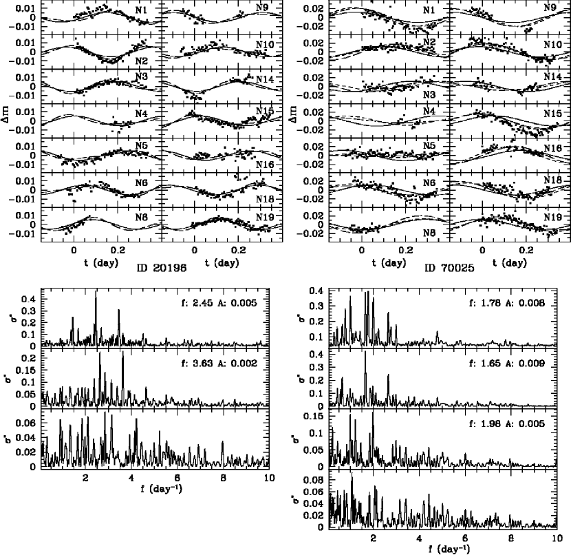
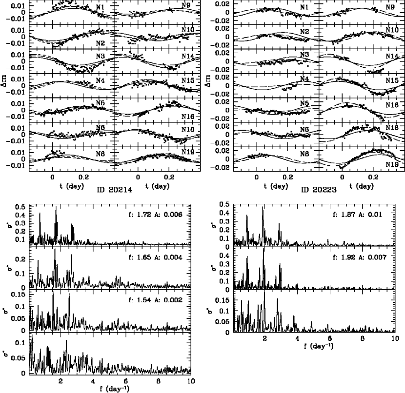
Early F-type stars containing multiple frequencies with periods of 0.4 to 3 days and 0.01 to 0.1 mag V-band amplitudes typify the $\gamma$ Doradus class (Krisciunas, 1998; Kaye et al., 1999). The pulsation mechanism is thought to arise from high-order, low-degree, nonradial gravity modes. The light curves for stars 70025, 20196, 20223, and 20214 show evidence of $\gamma$ Doradus variability. We identify multiple frequencies using the successive least-squares spectral analysis technique of Vaníc̆ek (1969, 1971) that is commonly applied to analyzing pulsating variables (Henry et al., 2005). Applying the spectral analysis to all the cluster variables, these four objects have unique signatures that set them apart from the others. For a majority of cluster variables, only the fundamental and harmonics exist in the light curve, whereas for the four $\gamma$ Doradus candidates, multiple frequencies exist that are not integer fractions of the fundamental.

Figures 14 and 15 present the light curves for the $\gamma$ Doradus candidates along with the best-fit light curve models in the upper parts of the figures. Each panel shows a single night’s data and the lines represent models of the variability with successively increased number of frequencies as identified in the spectral analysis. The solid line shows the first detected frequency fit to the data, the long-dashed line gives a two-component fit, and the short-dashed line gives a three-component fit. Figures 14 and 15 show the Vaníc̆ek (1971) optimum spectra statistic of the light curve as a function of frequency in the lower parts of the figures. The panels show successive identification of the frequencies present in the light curve from top to bottom. If a confident frequency is present, the frequency and its amplitude is noted in the upper right hand corner of the panel. We confidently detect a frequency when it appears in all variants of the light curves which we explain next.

When applying the spectral analysis to the cluster binary variables 60193 and 20534, their high amplitude, short period, and regularity allows us to detect numerous frequencies which are all harmonics of the fundamental. However, in the original light curves, lower significance frequencies were found very close to the dominant frequency detected. For binary stars this frequency splitting can occur if spot patterns on the close binaries appear or vary. The frequency splitting can also occur if the exposure timing is not accurate, or as we discovered during this study, it can result from corrections to the light curves to reduce systematic errors.

We find the procedure for removing the systematic trend in a light curve performs less than ideal in the presence of high amplitude variability. It slightly distorts the light curve enough to give rise to frequency splitting. The close frequency splitting is reduced when analyzing light curves without the seeing trend correction. In addition, the frequency splitting is further reduced by eliminating the last two nights of data. This suggests that the timing may be an issue over the baseline of observations. However, considering that the last two nights had some of the best seeing, it is not clear which of these two factors is the cause of the frequency splitting. Overall, the cleanest spectral analysis – which detects only harmonics – for stars 60193 and 20534 occurs without the seeing correction and without the last two nights of data. Thus, we define confidently detected frequencies in our $\gamma$ Doradus candidates as ones that are stable and detected in all variants of the light curves: the original light curves, light curves without the seeing correction, light curves without the last two nights of data, and light curves without the seeing correction and without the last two nights of data.

In addition to the multiple frequencies confidently identified in these 4 objects that are not harmonically related, these objects also occupy the upper main sequence in the CMD as expected for the typical spectral type for $\gamma$ Doradus variables. The large circles in Figure 1 designate their location in the CMD. However, the $\bv$ and estimated temperature for candidates 20214 and 20223 ($\bv\sim 0.42$ and $T_{eff}\sim 6700$ K) are redward and cooler than the empirically determined cool-edge boundary for $\gamma$ Doradus variables as defined by Henry et al. (2005) ($\bv$=0.38). The empirical cool edge of Henry et al. (2005) agrees well with the theoretical $\gamma$ Doradus instability strip as given by Warner et al. (2003) ($T_{eff}=6850$ K).

Alternatively, our effective temperatures may be systematically incorrect. The effective temperatures for these objects are estimated from the CMD and the best-fit cluster isochrone as described in Burke et al. (2004). Varying the metallicity of the cluster between -0.26$\leq[Fe/H]\leq$+0.13 while minimizing age, distance, and reddening to yield a best-fit isochrone to the observed CMD, yields a maximum $T_{eff}=6800$ K for these two stars. Reaching this high temperature requires an implausible $[Fe/H]=+0.13$. Thus, if objects 20214 and 20223 are confirmed as $\gamma$ Doradus stars they may represent the coolest known members of this class of variables. Also, the $\gamma$ Doradus candidates discovered in this study may represent the oldest known members of this class of variables given the $\sim$1 Gyr age for NGC 1245 (Martín & Rodríguez, 2002).

Confirming the $\gamma$ Doradus variables will require follow up spectroscopy and simultaneous light curves in several passbands. However, alternative models for the variability cannot reproduce the multiple frequencies that are not harmonically related. This is especially the case for objects 70025 and 20214 where we confidently detect three components Krisciunas (1998). Additionally, estimating the physical parameters of the stars from the best-fit isochrone we calculate the pulsation constant to range from -0.57$<\log Q<$-0.39 for our candidates. These values are consistent with the confirmed $\gamma$ Doradus variables of Handler & Shobbrook (2002). We used the strongest, first frequency detected when calculating the pulsation constant.

Assuming these four objects are $\gamma$ Doradus variables, we are able to measure the fraction of cluster members exhibiting this type of variability. Burke et al. (2004) statistically determine the cluster membership by characterizing the background star counts as a function of apparent magnitude from a control field at the outskirts of the field of view. The cluster membership as a function of magnitude is shown as Figure 9 in Burke et al. (2005). There is an estimated 45.9 cluster members for NGC 1245 between 15.83$<V<$16.27, the apparent magnitudes of our brightest and faintest $\gamma$ Doradus candidates. This corresponds to 2.88$<(M_{V})_{o}<$3.32 assuming a cluster distance modulus $(m-M)_{o}=12.27$ and extinction $A_{V}=0.68$. If all four objects are confirmed as $\gamma$ Doradus variables, then 8.7% of stars with properties similar to NGC 1245 in the above absolute magnitude range exhibit $\gamma$ Doradus variability. If none of the objects end up being $\gamma$ Doradus variables, then a null result implies $<6.5\%$ (95% confidence) of stars in this magnitude range exhibit $\gamma$ Doradus variability assuming we are 100% complete in detecting variability with amplitudes similar to the candidates.

Figure 14.— Light curves and power spectra for $\gamma$ Doradus candidates 20196 and 70025. In the light curve plots in the upper left and upper right, each panel shows a single night’s observations, with a label in the upper right corner of each panel identifying the night of the observing run, and an arbitrary x-axis zero point. The solid line shows a single component fit to the light curve, the long-dashed line gives a two-component fit, and the short-dashed line gives a three-component fit. The lower left and lower right panels show successive optimum spectra for 20196 and 70025. The top panel shows the spectra of the light curve which identifies the strongest frequency component present in the data. The component’s frequency and amplitude are labeled in the upper right corner of the panel. The successive panels from top to bottom show the spectra after taking into account the known constituents identified in the previous panels. The bottom panel gives the spectra after taking into account the two previously identified components. No stable component is identified in the bottom panel.

Figure 15.— Light curves and power spectra for $\gamma$ Doradus candidates 20214 and 20223. See caption of Figure 14 for description.

6. CONCLUSIONS

We have discovered 43 previously unknown variables in the field of NGC 1245, of which 14 are potential cluster members. Many of these variables are very low amplitude. Our method for determining relative photometry allows us to achieve sub-1% precision for stars brighter than $V=18$, enabling the characterization of such low amplitude variables. The techniques described in this paper can be readily applied to other long-term photometric data sets to determine the variability content of other surveys.

We roughly characterize the variables potentially belonging to the cluster. The light curves for objects 20534, 20176, 60193, 10462, and 60303 contain strong evidence for binarity. Object 10462 and 60303 are detached eclipsing binaries. If their membership in this cluster is confirmed, then the known ages and composition of these binaries offer opportunities for testing stellar models for cool stars.

The light curves for objects 20196, 70025, 20223, 20214 have evidence of multiple frequencies present and located near the main sequence turnoff. These objects are possible $\gamma$ Doradus candidates. Objects 20223 and 20214 would be the coolest ($T_{eff}\sim 6700$ K) known $\gamma$ Doradus variables if their status is verified. The standard solar metallicity and solar calibrated mixing length models of $\gamma$ Doradus variability do not predict pulsations in stars this cool (Dupret et al., 2004; Warner et al., 2003). Further exploration of parameter space may be necessary to fit these cool $\gamma$ Doradus candidates. Alternatively, the variability for these four objects can result from rapid rotation coupled with unstable spot patterns on the surface. Measuring the rotation rates and simultaneous light curves in multiple passbands for these objects would settle their classification.

The nature of potential cluster members 00210, 30338, 10429, 20513, and 20510 remain uncertain. These objects most likely result from ellipsoidal variability. Of the non-cluster objects, 10414, 30143, 20274, 20398, 10437, and 20065 are eclipsing binaries. The rest of the non-members cannot be well-characterized without knowledge of their absolute brightnesses and colors.

References

- Albrow et al. (2001) Albrow, M. D., Gilliland, R. L., Brown, T. M., Edmonds, P. D., Guhathakurta, P., & Sarajedini, A. 2001, ApJ, 559, 1060
- Binney & Merrifield (1998) Binney, J., & Merrifield, M. 1998, Galactic Astronomy (Princeton, NJ: Princeton University Press)
- Bramich et al. (2005) Bramich, D. M., et al. 2005, MNRAS, 360, 791H
- Burke et al. (2005) Burke, C. J., Gaudi, B. S., DePoy, D. L., & Pogge, R. W. 2005, AJ, submitted (astro-ph/0512207)
- Burke et al. (2004) Burke, C. J., Gaudi, B. S., DePoy, D. L., Pogge, R. W., & Pinsonneault, M. 2004, AJ, 127 2382
- Burke et al. (2002) Burke, C. J., DePoy, D. L., Gaudi, B. S., Marshall, J. L., & Pogge, R. W. 2002, in ASP Conf. Ser. 294: Scientific Frontiers in Research on Extrasolar Planets, eds. D. Deming and S. Seager (ASP: San Francisco), 379
- Dupret et al. (2004) Dupret, M. -A., Grigahcène, A., Garrido, R., Gabriel, M., & Scuflaire, R. 2004, A&AL, 414, 17
- Eyer & Blake (2005) Eyer, L., & Blake, C. 2005, MNRAS, 358, 30
- Handler & Shobbrook (2002) Handler, G. & Shobbrook, R. R. 2002, MNRAS, 333, 251
- Hargis, Sandquist & Bradstreet (2004) Hargis, J. R., Sandquist, E. L., & Bradstreet, D. H. 2004, BAAS, 205, 22.12
- Henry et al. (2005) Henry, G. W., Fekel, F. C., & Henry, S. M. 2005, AJ, 129, 2815
- Horne (2004) Horne, K. 2003, in ASP Conf. Ser. 294, Scientific Frontiers in Research on Extrasolar Planets, ed. D. Deming & S. Seager (San Francisco: ASP), 361
- Hidas et al. (2005) Hidas, M. G., et al. 2005, MNRAS, 360, 703
- Kaluzny et al. (1998) Kaluzny, J., Stanek, K. Z., Krockenberger, M., Sasselov, D. D., Tonry, J. L., & Mateo, M., 1998, AJ, 115, 1016
- Kaye et al. (1999) Kaye, A. B., Handler, G., Krisciunas, K., Poretti, E., & Zerbi, F. M. 1999, PASP, 111, 840
- Krisciunas (1998) Krisciunas, K. 1998, IAUS, 185, 339
- Martín & Rodríguez (2002) Martín, S. & Rodríguez, E. 2002, in Radial and Nonradial Pulsations as Probes of Stellar Physics, ed. C. Aerts, T. R. Bedding, & J. Christensen-Dalsgaard, PASPC, 259, 152
- Mizerski & Bejger (2002) Mizerski, T., & Bejger, M. 2002, acta , 52, 61
- Mochejska et al. (2004) Mochejska, B. J., Stanek, K. Z., Sasselov, D. D., Szentgyorgyi, A. H., Westover, M., & Winn, J. N. 2004, AJ, 128, 312
- Mochejska et al. (2002) Mochejska, B. J., Stanek, K. Z., Sasselov, D. D., & Szentgyorgyi, A. H. 2002, AJ, 123, 3460
- Mochejska et al. (2005) Mochejska, B. J., et al. 2005, astro-ph/0501145
- Rucinski (1994) Rucinski, S. M. 1994, PASP, 106, 462
- Schwarzenberg-Czerny (1996) Schwarzenberg-Czerny, A. 1996, ApJ, 460, L107
- Skrutskie et al. (1997) Skrutskie, M. F., et al. 1997, in The Impact of Large-Scale Near-IR Sky Surveys, eds. F. Garzon, N. Epchtein, A. Omont, B. Burton, & P. Persi (Dordrecht: Kluwer), 25 First citation in article — NASA ADS
- Sterken & Jaschek (1996) Sterken, C. & Jaschek, C. 1996, Light Curves of Variable Stars - a pictoral atlas (Cambridge, Great Britain: Cambridge University Press)
- Stetson (1996) Stetson, P. B. 1996, PASP, 108, 851
- Street et al. (2003) Street, R. A., et al. 2003, MNRAS, 340, 1287
- Vaníc̆ek (1969) Vaníc̆ek, P. 1969, Ap&SS, 4, 387
- Vaníc̆ek (1971) Vaníc̆ek, P. 1971, Ap&SS, 12, 10
- von Braun et al. (2005) von Braun, K., Lee, B. L., Seager, S., Yee, H. K. C., Mallén-Ornelas, G., & Gladders, M. D. 2005, PASP, 117, 141
- Warner et al. (2003) Warner, P. B., Kaye, A. B., & Guzik, J. A. 2003, ApJ, 593, 1049
- Yi et al. (2001) Yi, S., Demarque, P., Kim, Y. C., Lee, Y. W., Ree, C. H., Lejeune, T., & Barnes, S. 2001 ApJS, 136, 417