Accelerating universe in scalar tensor models - confrontation of theoretical predictions with observations.

Abstract

Aims. To study the possibility of appearance of accelerated universe in scalar tensor cosmological models

Methods. We consider scalar tensor theories of gravity assuming that the scalar field is non minimally coupled with gravity. We use this theory to study evolution of a flat homogeneous and isotropic universe. In this case the dynamical equations can be derived form a point like Lagrangian. We study the general properties of dynamics of this system and show that for a wide range of initial conditions such models lead in a natural way to an accelerated phase of expansion of the universe. Assuming that the point like Lagrangian admits a Noether symmetry we are able to explicitly solve the dynamical equations. We study one particular model and show that its predictions are compatible with observational data, namely the publicly available data on type Ia supernovae, the parameters of large scale structure determined by the 2-degree Field Galaxy Redshift Survey (2dFGRS), the measurements of cosmological distances with the Sunyaev-Zel’dovich effect and the rate of growth of density perturbations

Results. It turns out that this model have a very interesting feature of producing in a natural way an epoch of accelerated expansion. With an appropriate choice of parameters our model is fully compatible with several observed characteristics of the universe

1 Introduction

Recent observations of the type Ia supernovae, Gamma Ray Bursts, and CMB anisotropy indicate that the total matter-energy density of the universe is now dominated by some kind of dark energy (Riess & al. (1998); Riess (2000); Riess & al. (2004)). The origin and nature of this dark energy is not yet known (Zeldovich (1967); Weinberg (1989)).

In the last several years a new class of cosmological models has been proposed. In these models the standard cosmological constant $\Lambda$-term is replaced by a dynamical, time-dependent component - quintessence or dark energy - that is added to baryons, cold dark matter (CDM), photons and neutrinos. The equation of state of the dark energy is given by $w_{\phi}\equiv p_{\phi}/\rho_{\phi}$, where $p_{\phi}$ and $\rho_{\phi}$ are, respectively, the pressure and energy density, and $-1\leq w_{\phi}<0$, what implies a negative contribution to the total pressure of the cosmic fluid. When $w_{\phi}=-1$, we recover a constant $\Lambda$-term. One of the possible physical realizations of quintessence is a cosmic scalar field (Caldwell, Dave & Steinhardt (1998)), which induces dynamically a repulsive gravitational force, causing an accelerated expansion of the Universe, as recently discovered by observations of distant type Ia supernovae (SNIa) (Riess & al. (1998, 2004)) and confirmed by the WMAP observations (Spergel & al. (2003)).

The existence of a considerable amount of dark energy leads to at least two theoretical problems: 1) why only recently dark energy started to dominate over matter, and 2) why during the radiation epoch the density of dark energy is vanishingly small in comparison with the energy density of radiation and matter (fine tuning problem). The fine tuning problem can be alleviated by considering models of dark energy that admit so called tracking behavior (Steinhardt, Wang & Zlatev ). In such models, for a wide class of initial conditions, equation of state of dark energy tracks the equation of state of the background matter and radiation (Steinhardt, Wang & Zlatev ; Zlatev, Wang & Steinhardt (1999)). All these circumstances stimulated a renewed interest in the generalized gravity theories, and prompted consideration of a variable $\Lambda$ term in more general classes of theories, such as the scalar tensor theories of gravity (Perrotta, Baccigalupi & Matarrese (2000)). One of the additional advantages of appealing to these theories is that they open new prospective in the scenario of a decaying dark energy, since the same field that is causing the time (and space) variation of the dark energy is also causing the Newton’s constant to vary.

In this paper we consider cosmological models in a non minimally coupled scalar tensor theory of gravitation. We assume that the universe is homogeneous and isotropic and its geometry is described by the Friedman-Robertson-Walker line element. For the reason of simplicity we consider only the case of flat universe. In this case the scalar field depends only on time and the dynamical equations that describe evolution of the geometry and the scalar field can be derived form a point like Lagrangian. We derive the general set of dynamical equations and discuss their basic properties. When we require that the point like Lagrangian admits an additional Noether symmetry the dynamical equations can be explicitly integrated. In particular we consider a model with the scalar field potential of the form $V(\phi)=V_{0}\phi^{4}$ and we analyze its dynamics. Finally to compare predictions of our model with observations we concentrate on the following data: the publicly available data on type Ia supernovae, the parameters of large scale structure determined by the 2-degree Field Galaxy Redshift Survey (2dFGRS), and measurements of cosmological distances with the Sunyaev-Zel’dovich effect. We show that our model is compatible with these observational data.

Our paper is organized as follows: in Sec. 2 we present our model and discuss its basic properties. In Sec. 3 we confront predictions of our model with observational data, Sec. 4 is devoted to the discussion of evolution of density perturbations in our model and finally in Sec. 5 we present our conclusions.

2 Model description

Let us consider the general action of a scalar field $\phi$ non minimally coupled with gravity when there is no coupling between matter and $\phi$

$${\cal A}=\int_{T}\sqrt{-g}\left(F(\phi)R+\frac{1}{2}g^{\mu\nu}\phi_{,\mu}\phi_{,\nu}-V(\phi)+{\cal L}_{m}\right)d^{4}x\,,$$ (1)

where $F(\phi),\leavevmode\nobreak\ V(\phi)$ are two generic functions representing the coupling of the scalar field with geometry and its potential energy density respectively, $R$ is the curvature scalar, ${\displaystyle\frac{1}{2}g^{\mu\nu}\phi_{,\mu}\phi_{,\nu}}$ is the kinetic energy of the scalar field $\phi$ and ${\cal L}_{m}$ describes the standard matter content. In units such that $8\pi G_{N}=\hbar=c=1$, where $G_{N}$ is the Newtonian constant, we recover the standard gravity when $F=-\displaystyle{1\over 2}$, while in general the effective gravitational coupling $G_{eff}=-{1\over{2F}}$. Here we would like to study the simple case of a homogeneous and isotropic universe, what implies that the scalar field $\phi$ depends only on time. It turns out that in the flat Friedman-Robertson-Walker cosmologies, the action in Eq. (1) reduces to the pointlike Lagrangian

$${\cal L}=6Fa\dot{a}^{2}+6F^{\prime}\dot{\phi}a^{2}\dot{a}+a^{3}\left({1\over 2}\dot{\phi}^{2}-V(\phi)\right)-Da^{-3(\gamma-1)}\,,$$ (2)

where $a$ is the scale factor and prime denotes derivative with respect to $\phi$, while dot denotes derivative with respect to time. Moreover, the constant D is defined in such a way that the matter density $\rho_{m}$ is expressed as $\rho_{m}=D(a_{o}/a)^{3\gamma}$, where $1\leq\gamma\leq 2$. The effective pressure and energy density of the $\phi$-field are given by

$$p_{\phi}=\frac{1}{2}\dot{\phi}^{2}-V(\phi)-2(\ddot{F}+2H\dot{F})\,,$$ (3)

$$\rho_{\phi}=\frac{1}{2}\dot{\phi}^{2}+V(\phi)+6H\dot{F}\,,$$ (4)

where $H=\displaystyle{{\dot{a}}\over a}$ is the Hubble constant. These two expressions, even if not pertaining to a conserved energy-momentum tensor, define an effective equation of state $w_{\phi}=\displaystyle{p_{\phi}\over\rho_{\phi}}$, which drives the late time behavior of the model. The field equations derived from Eq. (2) are the same ones which would come from the field equations derived from Eq. (1) when homogeneity and isotropy is imposed, that is

$$H^{2}=-\frac{1}{2F}\left(\frac{\rho_{\phi}}{3}+\frac{\rho_{m}}{3}\right)\,,$$ (5)

$$2\dot{H}+3H^{2}=\frac{1}{2F}(p_{\phi}+p_{m})\,,$$ (6)

and

$$\ddot{\phi}+3H\dot{\phi}+6(\dot{H}+2H^{2})F^{\prime}+V^{\prime}=0\,.$$ (7)

The scalar tensor theory with the scalar field non minimally coupled to gravity provides a wide framework to study cosmological models. The function $F(\phi)$ that describes the coupling between the scalar filed and gravity is influencing not only the evolution of the cosmological scale factor and the scalar field itself but also determines the strength of gravitational interactions. In this paper we consider only the simple case of a homogeneous and isotropic flat universe filled in with a scalar field (quintessence) and pressureless matter, i.e., $p_{m}=0$ (dust). That is, strictly speaking, our model describes the evolution of the universe only after the matter-radiation decoupling. The scalar field which appears in our model is treated as quintessence. To discuss the changing influence of the scalar field on the evolution of the universe and the effective equation of state of quintessence, we set $x\equiv\displaystyle{{\dot{\phi}}^{2}\over 2V}$, and $\displaystyle x_{1}\equiv{\dot{F}\over V}$, we find that

$$w_{\phi}={p_{\phi}\over\rho_{\phi}} = {x-1+2x_{1}\left({\dot{V}\over V}+2H\right)-2\dot{x}_{1}\over x+1+6Hx_{1}}\,.$$ (8)

The parameter $x$ measures the ratio of the kinetic energy relative to the potential energy of the scalar field. In the non minimally coupled case it is possible to invert the Eq.(8) and we get that

$$x={\rho_{\phi}(1+w_{\phi})+2\left(\ddot{F}-H\dot{F}\right)\over\rho_{\phi}(1-w_{\phi})-2\left(\ddot{F}+5H\dot{F}\right)}\,.$$ (9)

When the coupling function $F$ is a constant we recover the relation $x\displaystyle={1+w_{\phi}\over 1-w_{\phi}}$ that holds in the minimally coupled case. When $w_{\phi}<0$ the quintessence contributes negative pressure, this occurs when

$$x<1+2\left[\dot{x}_{1}-x_{1}\left({\dot{V}\over V}+2H\right)\right],$$ (10)

while the inequalities

$$x \geq \dot{x}_{1}-x_{1}\left({\dot{V}\over V}+5H\right)\,,$$ (11)

$$x < \dot{x}_{1}-x_{1}\left({\dot{V}\over V}+5H\right)\,,$$ (12)

correspond to the standard quintessence $(w_{\phi}\geq-1)$ and superquintessence respectively $(w_{\phi}<-1)$. If both $F(\phi)$ and $V(\phi)$ are known, it is possible to describe, in the parameter space, the transition between standard quintessence and superquintessence. Let us now introduce the concept of an effective cosmological constant $\Lambda_{eff}$. Using Eq.(5) it is natural to define the effective cosmological constant as $\Lambda_{eff}=-\displaystyle{\rho_{\phi}\over{2F}}$. With this definition we can rewrite Eq.(5) as

$$3H^{2} = G_{eff}\rho_{m}+\Lambda_{eff}\,.$$ (13)

Introducing the standard Omega parameters by

$$\Omega_{m}=-{\rho_{m}\over{6FH^{2}}},\quad\Omega_{\phi}={\Lambda_{eff}\over{3H^{2}}}=-{\rho_{\phi}\over{6FH^{2}}}\,,$$

we get that as usual

$$\Omega_{m}+\Omega_{\phi}=1\,.$$ (14)

¿From the definition of $\rho_{\phi}$ and $p_{\phi}$ and the generalized Klein-Gordon equation it follows that

$$\dot{\rho}_{\phi}+3H\left(p_{\phi}+\rho_{\phi}\right)=-6H^{2}\dot{F},$$ (15)

and

$$\dot{\Lambda}_{eff}+\dot{G}_{eff}\rho_{m}=-3HG_{eff}\left(p_{\phi}+\rho_{\phi}\right).$$ (16)

These equations play a role of the continuity equations for $\rho_{\phi}$ and $\Lambda_{eff}$.
We will show later on that asymptotically for large time $\dot{G}_{eff}$ tends to zero, then $w_{\phi}$ determines the late time scaling of $\Lambda_{eff}$, and actually we have that

$${\dot{\Lambda}_{eff}\over\Lambda_{eff}}\approx-3\tilde{H}\left(1+w_{\phi}\right),$$ (17)

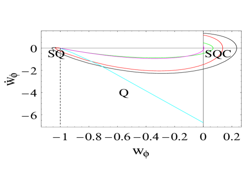
Figure 1: Rate of change of the equation of state as measured by ${\dot{w}}_{\phi}$ versus the $w_{\phi}$ parameter. We see that together with the superquintessence region $w_{\phi}<-1$, (SQ), there appears also a superquintessence connected region (SQC) with an equation of state $w_{\phi}>0$. The blue straight line corresponds, indeed, to values of parameters such that we observe neither a superquintessence expansion, nor a stiff matter behaviour.

where $\tilde{H}$ is the asymptotic value of $H$. It turns out that if at large $t$, $\tilde{H}$ is constant and $\neq 0$, than asymptotically $w_{\phi}\rightarrow-1$. Let us note that such a transition to the asymptotical value is responsible for the accelerated expansion. Even if we start from a dust or other stiff equation of state $w_{\phi}$ converges towards $-1$, as it is shown in Fig.1. Actually it turns out that together with the superquintessence region $w_{\phi}<-1$, (SQ), there exists also a superquintessence connected region (SQC) with an equation of state $w_{\phi}>0$. The blue straight line corresponds, indeed, to the values of parameters such that we observe neither a superquintessence expansion, nor a stiff matter behaviour.

2.1 Exact solutions through Noether theorem

To find exact solutions in the framework of the non minimally coupled models we assume that the pointlike Lagrangian possesses a Noether symmetry (for a detailed exposition of this technique which we closely follow here and interesting examples see (Capozziello & al. (1996))). This means that we require the existence of a Noether vector field along which the Lie derivative of the Lagrangian is zero. This requirement restricts the possible coupling and the form of the potential. In fact the additional Noether symmetry exists when

$$V=V_{0}(F(\phi))^{p(s)}\,,$$ (18)

where $V_{0}$ is a constant and

$$p(s)=\frac{3(s+1)}{2s+3}\,,$$ (19)

where $s$ is a real number, and when the coupling $F(\phi)$ satisfies the following differential equation

$$d_{1}F^{\prime\prime}F^{2}+d_{2}F^{\prime 4}+d_{3}F^{\prime 2}F+d_{4}F^{2}=0,$$ (20)

and the coefficients are functions of the parameter $s$,

$$d_{1}={2s+3\over 2}\,,$$ (21)

$$d_{2}=3s(s+1)(s+2)\,,$$ (22)

$$d_{3}=-\frac{1}{4}(s+1)(8s^{2}+16s+3)\,,$$ (23)

$$d_{4}=\frac{s(2s+3)^{2}}{12}\,.$$ (24)

A particular solution which indeed turns out to be quite interesting is of the form

$$F=\xi(s)(\phi+\phi_{0})^{2}\,,$$ (25)

where

$${\displaystyle\xi(s)=\frac{(2s+3)^{2}}{48(s+1)(s+2)}}\,,$$ (26)

and $\phi_{0}$ is a constant. The parameter $s$ labels then the class of Lagrangians which admit a Noether symmetry. Let us note that the form of the coupling given by (25) is quite relevant from the point of view of fundamental physics. Not all the values of $s$ are allowed however. From the expressions (18) and (26) it follows that the cases when $s=-1$, $s=-3/2$, $s=-2$ are special and they should be treated independently. Through Eq. (18) it is possible to recover the inverse power-law potentials, while the case $s=0$ as we will see later is special and it corresponds to the square hyperbolic sine potential. Both these potentials are usually assumed ad hoc to obtain certain asymptotic behavior of the energy density of the quintessence field (Peebles & Ratra (1988); Urena-Lopez & Matos (2000)), while here they emerge naturally from the imposed Noether symmetry. Once the general solution of Eq.(20) is found, what automatically specifies the form of the potential, and a generic value of $s$ is considered, it is possible to explicitly find the Noether symmetry and to introduce new dynamical variables associated with this symmetry (for details see (Capozziello & al. (1996))). Using the new dynamical variables it is then possible to solve the corresponding Lagrange equations and finally by inverting them we obtain the sought after $a(t)$ and $\phi(t)$. The final result can be written in the form

$$a(t)=A(s)\left(B(s){(s+3)^{2}\over{6(s+6)}}t^{3\over{s+3}}+{D\over{\Sigma_{0}}}\right)^{{s+1}\over s}t^{{2s^{2}+6s+3}\over{s(s+3)}}\,,$$ (27)

$$\phi(t)=C(s)\left(-{V_{0}\over\gamma(s)}B(s)t^{3\over{s+3}}+{D\over\Sigma_{0}}\right)^{-{{2s+3}\over 2s}}t^{-{(2s+3)^{2}\over{2s(s+3)}}}-\phi_{0}\,,$$ (28)

where $D$ is the matter density constant, $\Sigma_{0}$ is a constant of the motion resulting from the Noether symmetry, $V_{0}$ is the constant that determines the scale of the potential, $\phi_{0}$ is a constant that determines the initial value of the scalar field and the other constants $A(s)$, $B(s)$, $C(s)$, and $\gamma(s)$ are given in the appendix. As it is apparent from Eq.(27) and Eq.(28) for a generic value of $s$ both the scale factor $a(t)$ and the scalar field $\phi(t)$ have a power law dependence on time. It is also clear that there are two additional particular values of $s$, namely $s=0$ and $s=-3$ which should be treated independently. In this paper we concentrate on the case $s=-3$ which provides, as will be shown shortly, an interesting class of models.

2.1.1 The case of quartic potentials: analysis of the solution

When $s=-3$ the general solutions given by (27) and (28) lose their meaning. To find $a(t)$ and $\phi(t)$ in this case it is necessary to use the general procedure as described in (Capozziello & al. (1996)). From Eq.(18) and Eq.(25) it follows that in this case $F=\frac{3}{32}\phi^{2}$, and $V(\phi)=V_{0}\phi^{4}$ where we have set $\phi_{0}=0$ and $V_{0}$ denotes a constant. This case is particularly interesting since the resulting self–interaction potential is used in finite temperature field theory. In fact, it seems that the quartic form of the potential is required in order to implement the symmetry restoration in several Grand Unified Theories. Just for this reason we limit our analysis to this special case, and we will show that it provides an accelerated expansion of the universe. We reserve to a forthcoming paper the study of the other cases. As in the general case once we have the functions $F(\phi)$ and $V(\phi)$ that allow a Noether symmetry it is possible to explicitly find it and effectively solve the Lagrange equations. Performing this procedure we finally get

$$a(t)=\alpha_{0}e^{{-\alpha_{1}t\over 3}}\left[{\left(e^{\alpha_{1}\,t}-1\right)\,+\alpha_{2}\,t+\alpha_{3}}\right]^{\frac{2}{3}}\,,$$ (29)

$$\phi(t)=\phi_{0}\sqrt{e^{\alpha_{1}t}\over\left(e^{\alpha_{1}\,t}-1\right)\,+\alpha_{2}\,t+\alpha_{3}}\,,$$ (30)

where $\alpha_{0}$, $\alpha_{1}$, $\alpha_{2}$ $\alpha_{3}$ and $\phi_{0}$ are integration constants. They are related to the initial matter density, $D$, and the scale of the potential $V_{0}$ by $D={{V_{0}}\over 16}\alpha_{0}^{3}\phi_{0}^{2}\alpha_{1}\alpha_{2}$, which implies that they cannot be zero. The case $V_{0}=0$ has to be treated separately. It turns out that the constants $\alpha_{3}$, $\phi_{0}$ and $\alpha_{0}$ have an immediate physical interpretation: $\alpha_{0}$, and $\alpha_{3}$ are connected to the value of the scale factor at $t=0$, actually $a(0)=(\alpha_{3})^{2\over 3}\alpha_{0}$. Moreover $\alpha_{3}$ can be selected in such a way that at a sufficiently early epoch the universe is matter dominated. This requires that $\alpha_{3}$ be sufficiently small, for example, that $\alpha_{3}\in[0.001,0.01]$. The constants $\alpha_{3}$ and $\phi_{0}$ are connected to the initial value of the scalar field $\phi(0)=\displaystyle{\phi_{0}\over\sqrt{\alpha_{3}}}$ and therefore they determine the initial value of the effective gravitational constant $G_{eff}(0)=-\displaystyle{{16\alpha_{3}}\over{3\phi_{0}^{2}}}$. Let us note that an attractive gravity is recovered when $\phi_{0}$ is a pure imaginary number. Without compromising the general nature of the problem we can set, for example $\phi_{0}=\imath$. This choice does not violate the positivity of energy density of the scalar field or the weak energy condition. To determine the integration constants $\alpha_{1}$, $\alpha_{2}$, $\alpha_{3}$ and $\phi_{0}$ we follow the procedure used in (Demianski & al. (2005)), and we set the present time $t_{0}=1$. That is to say that we are using the age of the universe, $t_{0}$, as a unit of time. Because of our choice of time unit the expansion rate $H(t)$ is dimensionless, so that our Hubble constant is not the same as the $H_{0}$ that appears in the standard FRW model, measured in $kms^{-1}Mpc^{-1}$: we then set ${\widehat{H}}_{0}=H(1)$. Using (29) we get

$$H(1)={\widehat{H}}_{0}=-{\alpha_{1}\over 3}+{2\over 3}{{{\alpha_{1}}e^{\alpha_{1}}+\alpha_{2}}\over{e^{\alpha_{1}}+\alpha_{2}+\alpha_{3}-1}}\,,$$

which we use to find $\alpha_{2}$ in the form

$$\alpha_{2}={{e^{\alpha_{1}}(\alpha_{1}-3{\widehat{H}}_{0})+(\alpha_{3}-1)(3{\widehat{H}}_{0}+\alpha_{1})}\over{3{\widehat{H}}_{0}+\alpha_{1}-2}}\,.$$

With this choice of time the scale factor, the scalar field and the expansion rate assume the final form

$$a(t)=a_{0}e^{-\frac{\alpha_{1}t}{3}}\left(e^{\alpha_{1}t}+{{e^{\alpha_{1}}(\alpha_{1}-3{\widehat{H}}_{0})+(\alpha_{3}-1)(3{\widehat{H}}_{0}+\alpha_{1})}\over{3{\widehat{H}}_{0}+\alpha_{1}-2}}t+\alpha_{3}-1\right)^{2/3}\,,$$

$$\phi(t)=\phi_{0}\sqrt{\frac{e^{\alpha_{1}t}}{e^{\alpha_{1}t}-{{e^{\alpha_{1}}(\alpha_{1}-3{\widehat{H}}_{0})+(\alpha_{3}-1)(3{\widehat{H}}_{0}+\alpha_{1})}\over{3{\widehat{H}}_{0}+\alpha_{1}-2}}t+\alpha_{3}-1}}\,,$$ (31)

$$H(t)=\left\{\alpha_{1}\left(\alpha_{1}+2e^{\alpha_{1}}\right)+e^{\alpha_{1}t}\alpha_{1}\left(3{\widehat{H}}_{0}+\alpha_{1}-2\right)+3{\widehat{H}}_{0}\left(\alpha_{1}-2e^{\alpha}_{1}+2\right)\right.$$ (32)

$$\left.-\left(\alpha_{1}^{2}+3{\widehat{H}}_{0}\left(\alpha_{1}+2\right)\right)\alpha_{3}+\left[\left(-1-e^{\alpha}_{1}\right)\alpha_{1}^{2}+\alpha_{3}\alpha_{1}^{2}+3\left(-1+e^{\alpha}_{1}+\alpha_{3}\right){\widehat{H}}_{0}\alpha_{1}\right]t\right\}\times$$

$$\left\{\{3e^{\alpha_{1}t}\left(3{\widehat{H}}_{0}+\alpha_{1}-2\right)-\left(\alpha_{3}-1\right)\left(3{\widehat{H}}_{0}(t-1)+\alpha_{1}(t-1)+2\right)+e^{\alpha}_{1}(\alpha_{1}-3{\widehat{H}}_{0})t\right\}^{-1}\,.$$

Let us remind that $t$ is now varying from $0$ to $1$ and $t=1$ corresponds to the present moment. The parameters ${\widehat{H}}_{0}$ and $\alpha_{1}$ admit a simple physical interpretation. Actually ${\widehat{H}}_{0}$ is the present value of the Hubble constant measured in our unit of time, while $\alpha_{1}$ drives the early time and the asymptotical behavior of $a(t)$ and $\phi(t)$. For $t\ll{1\over\alpha_{1}}$ we have

$$a(t) \sim \left[(\alpha_{1}+\alpha_{2}-{\alpha_{1}\alpha_{2}\over 2})t+\alpha_{3}\right]^{2\over 3}$$ (33)

$$\phi(t) \sim \left[(\alpha_{1}+\alpha_{2}-\alpha_{1}\alpha_{3})t+\alpha_{3}\right]^{-{1\over 2}}.$$ (34)

Later at larger $t$, $a(t)$ reaches an intermediate stage, when it evolves as $a(t)\sim t^{2\over 3}e^{-{\alpha_{1}t\over 3}}$ (dumped dust) , and has a de Sitter behavior $a(t)\sim e^{{\alpha_{1}t}\over 3}$ for $t\rightarrow\infty$.

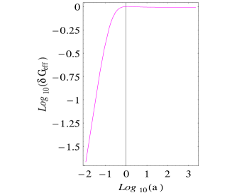
Figure 2: Plot of ${\log}_{10}\delta G_{eff}=\displaystyle{\log}_{10}{G_{eff}\over G_{eff}(t_{0})}$ versus ${\log}_{10}a$ . The vertical bar marks ${\log}_{10}a_{0}$.

It is interesting to note that $w_{\phi}$ is representing an equation of state, in the usual sense, of the effective cosmological constant $\Lambda_{eff.}$. In Figs.(3,4,5) we show the time dependence of $w_{\phi}$: we see that this equation of state can admit a superquintessence behavior ($w<-1$), just as an effect of the transition toward $w\rightarrow-1$.

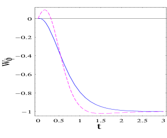
Figure 3: Time dependence of $w_{\phi}$, for two different values of the parameters. Actually the solid curve corresponds to $\alpha_{1}=2.5$, and ${\widehat{H}}_{0}=0.95$, while the dashed one corresponds to $\alpha_{1}=3$, and ${\widehat{H}}_{0}=1$. We see that even though they both produce accelerated expansion, only the second one gives rise to super acceleration.

Figure 4: Parametric plot of $w_{\phi}$ as a function of the acceleration; we see the transition from the accelerated to the decelerated expansion.

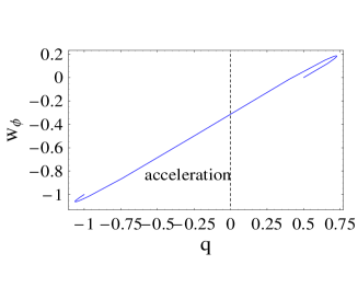
Figure 5: Parametric plot of $w_{\phi}$ with respect to the deceleration parameter $q=-{\ddot{a}\dot{a}\over a^{2}}$; again we see the transition from the accelerated to the decelerated expansion. Moreover, we see that if we consider the value $q\simeq-0.68$ obtained from the SNIa Gold Sample (Riess & al. (2004)) we obtain $w_{\phi}\leq-0.65$

We note that in the remote past as in the far future $w_{\phi}$ is constant: it mimics an almost dust equation of state ($w_{\phi}\approx 0$) in the far past and asymptotically behaves as a bare cosmological constant ($w_{\phi}\rightarrow-1$) as $t\rightarrow\infty$. Let us also mention that since both $\rho_{\phi}$ and $p_{\phi}$ depend on $F(\phi)$ through its time derivative and asymptotically $\phi(t)\sim{\rm constant}$ we asymptotically recover the minimally coupled case, with

$$\rho_{\phi_{\infty}} = \frac{1}{2}{{\dot{\phi}}_{\infty}}^{2}+V_{\infty}(\phi)=V_{0}\phi_{0}^{4}+{1\over 8}\phi_{0}^{2}e^{-2\alpha_{1}t}\,,$$ (35)

$$p_{\phi_{\infty}} = \frac{1}{2}{{\dot{\phi}}_{\infty}}^{2}-V_{\infty}(\phi)=-V_{0}\phi_{0}^{4}+{1\over 8}\phi_{0}^{2}e^{-2\alpha_{1}t}\,.$$ (36)

However, before reaching this asymptotic regime the total energy density $\rho_{\phi}$ is dominated by the coupling term $6H\dot{F}$. In conclusion of this section we present the traditional plot $\log{\rho_{\phi}}$ - $\log a$ compared with the matter density (see Fig. (6)). Interestingly we see that $\rho_{\phi}$ tracks the matter during the matter dominated era ( actually $a(t)\propto t^{2\over 3}$, and $w_{\phi}\sim 0$), and becomes dominant at late time. In Fig.(7) we plot the redshift behavior of the quintessence sound velocity; we see that $c_{s}<1$.

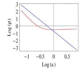
Figure 6: Plot of ${\log}_{10}\rho_{\phi}$ versus ${\log}_{10}a$. The vertical bar marks ${\log}_{10}a_{0}$. The solid blue straight line indicates the log-log plot of $\rho_{m}$ versus a.

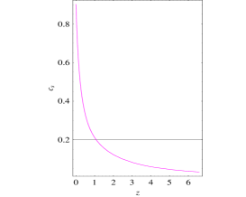
Figure 7: The redshift behavior of the quintessence sound velocity $c_{s}$.

2.1.2 A special case: asymptotic freedom at $t\simeq 0$

In this section we consider a special case when $\lim_{t\rightarrow 0}G_{eff}=0$, that is when $\lim_{t\rightarrow 0}\phi=\infty$ we have a sort of asymptotic freedom at $t=0$. First of all we note that such a case can be reached by setting $\alpha_{3}=0$, which also implies that $a(t=0)=0$, and the expressions for $a(t)$ and $\phi(t)$ become simpler. In comparison with the case $\alpha_{3}\neq 0$ the main difference concerns the behavior of the density $\rho_{\phi}$ with respect to the matter density, as shown in Fig. (8). Actually we note that the coupling $F(\phi)$ diverges as $t\rightarrow 0$, with its derivatives, more rapidly than $\rho_{m}$. However $\rho_{m}$ always dominates over the scalar field contribution to the density, that is over $\rho_{\phi}$.

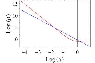
Figure 8: Plot of ${\log}_{10}\rho_{\phi}$ versus ${\log}_{10}a$ when there is asymptotic freedom at $t\simeq 0$ . The vertical line marks ${\log}_{10}a_{0}$. The solid blue straight line indicates the log-log plot of $\rho_{m}$ versus a.

It should be remembered that the early epoch $t\approx 0$ does not belong to the physical time domain of our model, since we are neglecting the contribution of radiation, and therefore the time behavior of $G_{eff}$ during the intermediate period is unknown. This is also the reason why we are not using any constraint on $G_{eff}$ from the nucleosynthesis. With respect to the other characteristic features this case is similar to that discussed above, as shown in the Fig. (9)

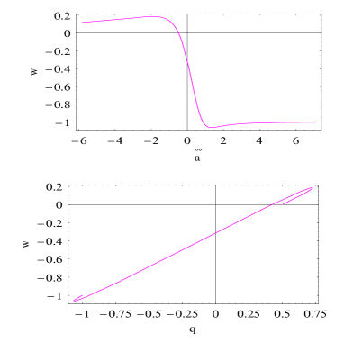
Figure 9: The same as in Figs (4,5)when there is asymptotic freedom at $t\simeq 0$ .

3 Observational data and predictions of our models

Above we discussed some general properties of our scalar field model of quintessence, stressing how it provides a natural mechanism for the observed accelerated expansion of the universe. To test viability of our model we compare its predictions with the available observational data. We concentrate mainly on two different kinds of observational data: some of them are all based on distance measurements, as the publicly available data on type Ia supernovae, the measurements of cosmological distances with the Sunyaev-Zel’dovich effect and radio-galaxies data, other are instead connected with the large scale structure, such as the parameters of large scale structure determined by the 2-degree Field Galaxy Redshift Survey (2dFGRS), and the gas fraction in clusters. Before we begin our analysis we note in Fig. 12 that for our model the transition redshift from a decelerating to an accelerating phase in the evolution of the universe falls very close to $z=0.5$, in agreement with recent results coming from the SNIa observations (Riess & al. (2004)).

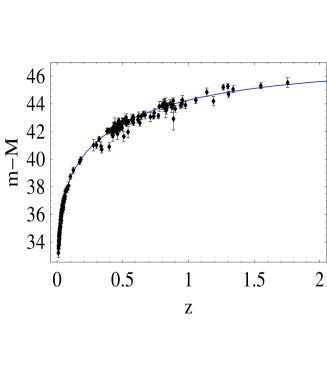
Figure 10: Observational data of the Gold Sample of SNIa (Riess et al. 2004) and the SNLS dataset (Astier & al. (2005)) fitted to our model. The solid curve is the best fit curve with ${\widehat{H}}_{0}=1.0^{+0.03}_{-0.04}$, $\alpha_{1}=2.9^{+0.2}_{-0.3}$, which corresponds to $\Omega_{{\rm\Lambda_{eff}}}=0.84_{-0.07}^{+0.06}$. We also get $h=0.68^{+.05}_{-.03}$.

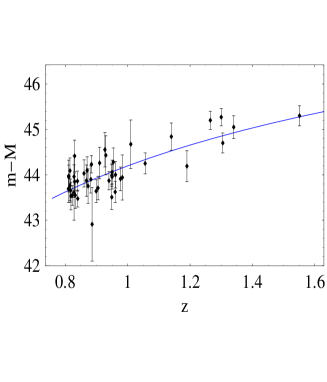
Figure 11: The same as in the Eq. (11) , but zooming on the high redshift SNIa.

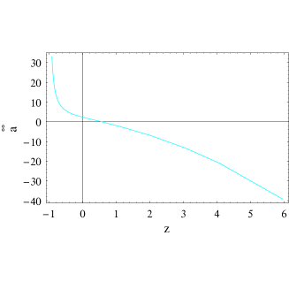
Figure 12: Behavior of the second derivative of the scale factor. Please note that the transition from a decelerating to an accelerating expansion occurs close to $z=0.5$, as predicted by recent observations of SNIa $z_{t}=0.46\pm 0.13$ (Riess & al. (2004)).

3.1 Constraints from recent SNIa observations

In recent years the confidence in type Ia supernovae as standard candles has been steadily growing. Actually it was just the SNIa observations that gave the first strong indication of an accelerating expansion of the universe, which can be explained by assuming the existence of some kind of dark energy or nonzero cosmological constant (Schmidt & al. (1998)). Since 1995 two teams of astronomers have been discovering type Ia supernovae at high redshifts. First results of both teams were published by Schmidt & al. (1998) and Perlmutter & al. (1999). Recently the High-Z SN Search Team reported discovery of 8 new supernovae in the redshift interval $0.3\leq z\leq 1.2$ and they compiled data on 230 previously discovered type Ia supernovae (Tonry et al. (2001)). Later Barris & al. (2004) announced the discovery of twenty-three high-redshift supernovae spanning the range of $z=0.34-1.03$, including 15 SNIa at $z\geq 0.7$ .
More recently Riess & al.  (2004) announced the discovery of 16 type Ia supernovae with the Hubble Space Telescope. This new sample includes 6 of the 7 most distant ($z>1.25$) type Ia supernovae. They determined the luminosity distance to these supernovae and to 170 previously reported ones using the same set of algorithms, obtaining in this way a uniform ”Gold Sample” of type Ia supernovae containing 157 objects. Finally just recently the Supernova Legacy Survey (SNLS) team presented the data collected during the first year of the SNLS program. It consists of 71 high redshift supernovae in the redshift range $z\in\left[0.2,\,\,1\right]$. This new SNLS sample is characterized by precise distance measurements of all the $71$ supernovae, so it can be used to build the Hubble diagram extending to $z=1$. The purpose of this section is to test our scalar field quintessence model by using the best SNIa data sets presently available. As a starting point we consider the gold sample compiled by (Riess & al. (2004)) to which we add the SNLS dataset. To constrain our model we compare through a $\chi^{2}$ analysis the redshift dependence of the observational estimates of the distance modulus, $\mu=m-M$, to the corresponding theoretical values. The distance modulus is generally defined by

$$m-M=5\log{D_{L}(z)}+5\log({c\over H_{0}})+25,$$ (37)

where $H_{0}$ is the standard Hubble constant, measured in $kms^{-1}Mpc^{-1}$, $m$ is the appropriately corrected apparent magnitude including reddening, K correction etc., $M$ is the corresponding absolute magnitude, and $D_{L}$ is the luminosity distance in Mpc. However, in scalar tensor theories of gravity it is important also to include in the Eq. (37) corrections, which describe the effect of the time variation of the effective gravitational constant $G_{eff}$ on the luminosity of high redshift supernovae. Actually, if the local value of $G_{eff}$ at the space time position of the most distant supernovae differs from $G_{N}$, this could in principle induce a change in the Chandrasekhar mass $M_{ch}\propto G^{-{3\over 2}}$. Some analytical models of the supernovae light curves predict that the peak luminosity is proportional to the mass of nickel produced during the explosion, which is a fraction of the Chandrasekhar mass. The actual fraction varies in different scenarios, but always the physical mechanism of type Ia supernovae explosion relates the energy yield to the Chadrasehkar mass. Assuming that the same mechanism for the ignition and the propagation of the burning front is valid for SNIa at high and low redshifts, it turns out that the predicted apparent magnitude will be fainter by a quantity (Gaztañaga & al. 2002 )

$$\Delta M_{G}={15\over 4}\log\left(G_{eff}\over G_{eff_{0}}\right).$$ (38)

Taking this into account the distance modulus becomes

$$m-M=5\log{D_{L}(z)}+5\log({c\over H_{0}})+25+\Delta M_{G}.$$ (39)

The presence of this correction actually allows one to test the scalar tensor theories of gravity (Gaztañaga & al. 2002 ; Uzan (2003)) using the SNIa data. For a general flat and homogeneous cosmological model the luminosity distance can be expressed as an integral of the Hubble function as follows:

$$D_{L}(z) = {c\over H_{0}}(1+z)\int^{z}_{0}{1\over H(\zeta)}d\zeta,$$ (40)

where $H(z)$ is the Hubble function expressed in terms of $z=a_{0}/a(t)-1$. Using Eqs. (38) and (40), which in our case can be integrated only numerically, we construct the distance modulus and perform the $\chi^{2}$ analysis on the complete data set. We obtain $\chi_{red}^{2}=1.7$ for 230 data points, and the best fit value is ${\widehat{H}}_{0}=1.0^{+0.03}_{-0.04}$, $\alpha_{1}=2.9^{+0.2}_{-0.3}$, which corresponds to $\Omega_{{\rm\Lambda_{eff}}}=0.73_{-0.07}^{+0.06}$. We also get $h=0.68^{+.05}_{-.03}$. Moreover we checked that any value of $\alpha_{3}\in[0.001,0.01]$ does not affect the determination of distances, so that in the following we set $\alpha_{3}=0.001$, being confident that such a choice does not alter the main results. In Fig (11) we compare the best fit curve with the observational data sets.

3.1.1 Dimensionless coordinate distance test

After having explored the Hubble diagram of SNIa, that is the plot of the distance modulus as a function of the redshift $z$, we want here to follow a very similar, but more general approach, considering as cosmological observable the dimensionless coordinate distance defined as :

$$y(z)=\int_{0}^{z}{\frac{1}{H(\zeta)}d\zeta}\ .$$ (41)

It is worth noting that $y(z)$ does not depend explicitly on $h$ so that any choice for $h$ does not alter the main result. Daly & Djorgovski (Daly & Djorgovski (2004)) have determined $y(z)$ for the SNIa in the Gold Sample of Riess et al. (Riess & al. (2004)) which represents the most homogeneous SNIa sample available today. Since SNIa allows to estimate $D_{L}$ rather than $y$, a value of $h$ has to be set. Fitting the Hubble law to a large set of low redshift ($z<0.1$) SNIa, Daly & Djorgovski (Daly & Djorgovski (2004)) have found that :

$$h=0.66\pm 0.08\ {\rm km\ s^{-1}\ Mpc^{-1}}\,,$$

which is consistent with our fitted value $h=0.66^{+.05}_{-.03}$. To enlarge the sample, Daly & Djorgovski added 20 further points on the $y(z)$ diagram using a technique of distance determination based on the angular dimension of radiogalaxies (Daly & Djorgovski (2004)). This extended sample that spans the redshift range $(0.1,1.8)$ has been obtained by homogenizing different kinds of measurements, affected by different systematics, so that the full sample may be used without introducing spurious features in the $y(z)$ diagram. However before using the dimensionless coordinate distance test we do not use the Daly & Djorgovski database directly, but, for the supernovae Gold Sample we first converted the distance modulus into $y(z_{i})$ using the Eq. (39) and the relation

$$D_{L}=\frac{c}{H_{0}}(1+z)y(z).$$

Here again $H_{0}$ is the standard FRW Hubble constant. To determine the best fit parameters, we define the following merit function :

$$\chi^{2}(\alpha_{1},{\widehat{H}}_{0})=\frac{1}{N-3}\sum_{i=1}^{N}{\left[\frac{y(z_{i};\alpha_{1},{\widehat{H}}_{0})-y_{i}}{\sigma_{i}}\right]^{2}}\,.$$ (42)

We obtain $\chi_{red}^{2}=1.19$ for 186 data points, and the best fit value is ${\widehat{H}}_{0}=0.98^{+0.05}_{-0.03}$, $\alpha_{1}=2.5^{+0.3}_{-0.2}$. In Fig (13) we compare the best fit curve with the observational data set.

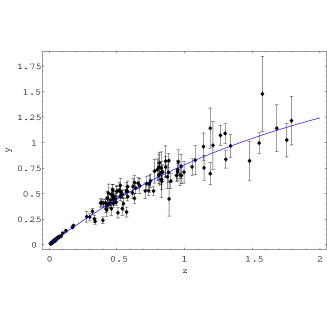
Figure 13: Observational Daly & Djorgovski database (Daly & Djorgovski (2004)) fitted to our model. The solid curve is the best fit curve with $\chi_{red}^{2}=1.19$ for 186 data points, and the best fit value is ${\widehat{H}}_{0}=1.00^{+0.05}_{-0.03}$, $\alpha_{1}=2.5^{+0.3}_{-0.2}$.

Daly & Djorgovski (Daly & Djorgovski (2004)) developed a numerical method for a direct determination of the expansion and acceleration rates, $H(z)$ and $q(z)$, from the data, just using the dimensionless coordinate distance $y(z)$, without making any assumptions about the nature or evolution of the dark energy. They actually use the equation

$$-q(z)\equiv\ddot{a}a/\dot{a}^{2}=1\leavevmode\nobreak\ +\leavevmode\nobreak\ (1+z)\leavevmode\nobreak\ (dy/dz)^{-1}(d^{2}y/dz^{2})\,,$$ (43)

valid for $k=0$. Equation (43) depends only upon the Friedman-Robertson-Walker line element and the relation $(1+z)=a_{0}/a(t)$. Thus, this expression for $q(z)$ is valid for any homogeneous and isotropic universe in which $(1+z)=a_{0}/a(t)$, and is therefore quite general and can be compared with any model to account for the acceleration of the universe. This new approach has the advantage of being model independent, but it introduces larger errors in the estimation of $q(z)$, because the numerical derivation is very sensitive to the size and quality of the data. An additional problem is posed by the sparse and not complete coverage of the $z$-range of interest. Measurement errors are propagated in the standard way leading to estimated uncertainties of the fitted values. In Fig. (14) we compare the $q(z)$ obtained by Daly & Djorgovski from their full data set with our best fit model.

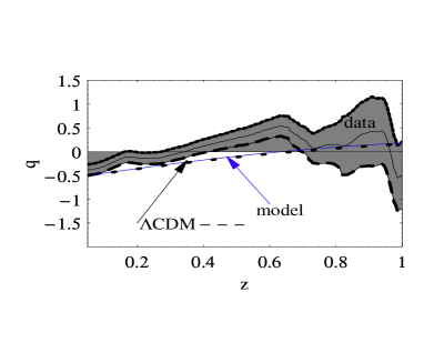
Figure 14: A first look at the allowed region for $q(z)$, obtained by Daly & Djorgovski from the full data set (shadow area). Approximated polynomial corresponding to a $z$-window $\Delta z=0.6$ is shown with the black thin solid line, with the black thick dashed lines are shown the approximated polynomial fitted to the smoothed data at $\pm 1\sigma$ range, and corresponding to a $z$-window $\Delta z=0.4$. The blue solid line shows the deceleration function, q(z), for our model corresponding to the the best fit values ${\widehat{H}}_{0}=1.00^{+0.05}_{-0.03}$, $\alpha_{1}=2.5^{+0.3}_{-0.2}$. It is compared to the corresponding function for the standard $\Lambda$CDM model with $\Omega_{M}=0.3$, $\Omega_{\Lambda}=0.7$.

3.2 The Sunyaev-Zeldovich/X-ray method

In this section we discuss how the parameters of our model can be also constrained by the angular diameter distance $D_{A}$ as measured using the Sunyaev-Zeldovich effect (SZE) and the thermal bremsstrahlung (X-ray brightness data) for galaxy clusters. Actually in a homogenous and isotropic cosmological model the angular diameter distance can be easily related to the coordinate distance leading to

$$D_{A} = {c\over H_{0}}{1\over(1+z)}\int_{0}^{z}{\frac{1}{H(\zeta)}d\zeta}.$$ (44)

Distance measurements using SZE and X-ray emission from the intracluster medium are based on the fact that these processes depend on different combinations of some parameters of the clusters (see Birkinshaw (1999) and references therein). The SZE is a result of the inverse Compton scattering of the CMB photons on hot electrons of the intracluster gas. The number of photons is preserved, but photons gain energy and thus a decrement of the temperature is generated in the Rayleigh-Jeans part of the black-body spectrum while an increment appears in the Wien region. We limit our analysis to the so called thermal or static SZE, which is present in all the clusters, neglecting the ${\it kinematic}$ effect, which is present only in clusters with a nonzero peculiar velocity with respect to the Hubble flow along the line of sight. Typically the thermal SZE is an order of magnitude larger than the kinematic one. The shift of temperature is:

$$\frac{\Delta T}{T_{0}}=y\left[x\,\mbox{coth}\,\left(\frac{x}{2}\right)-4\right],$$ (45)

where ${\displaystyle x=\frac{h\nu}{k_{B}T}}$ is a dimensionless variable, $T$ is the shifted radiation temperature, $T_{0}$ is the unperturbed CMB temperature and $y$ is the so called Compton parameter, defined as the optical depth $\tau=\sigma_{T}\int n_{e}dl$ times the energy gain per scattering:

$$y=\int\frac{k_{B}T_{e}}{m_{e}c^{2}}n_{e}\sigma_{T}dl.$$ (46)

In Eq. (46), $T_{e}$ is the temperature of the electrons in the intracluster gas, $m_{e}$ is the electron mass, $n_{e}$ is the number density of the electrons, and $\sigma_{T}$ is the cross section of Thompson electron scattering. We have used the condition $T_{e}\gg T_{0}$ ($T_{e}$ is of the order of $10^{7}\,K$ and $T_{0}$, is the CMB temperature $\simeq 2.7K$) and we assumed that the CMB temperature varies linearly with redshift what implies that after recombination the CMB radiation cools adiabatically with no injection of energy in the form of photons. In the low frequency regime of the Rayleigh-Jeans approximation we obtain

$$\frac{\Delta T_{RJ}}{T_{0}}\simeq-2y\,.$$ (47)

The next step to quantify the SZE decrement is to specify the model for the intracluster electron density and temperature distribution. The most commonly used model is the so called isothermal $\beta$ model of Cavaliere & Fusco Femiano . In this model

$$n_{e}(r)=n_{e_{0}}\left(1+\left(\frac{r}{r_{e}}\right)^{2}\right)^{-\frac{3\beta}{2}}\,,$$ (48)

$$T_{e}(r)=T_{e_{0}}\leavevmode\nobreak\ ,$$ (49)

where $n_{e_{0}}$ and $T_{e_{0}}$ are respectively the central electron number density and temperature of the intracluster electron gas, $r_{e}$ and $\beta$ are fitting parameters connected with the model (Sarazin (1988)). The relative temperature shift is given by

$$\frac{\Delta T}{T_{0}}=-\frac{2k_{B}\sigma_{T}T_{e_{0}}\,n_{e_{0}}}{m_{e}c^{2}}{\cdot}\Sigma\,,$$ (50)

where

$$\Sigma=\int^{\infty}_{0}\left(1+\left(\frac{r}{r_{c}}\right)^{2}\right)^{-\frac{3\beta}{2}}dl\,,$$ (51)

which depends only on the geometry and the extension of the cluster along the line of sight. In Eq.(51), $l$ is the coordinate along the line of sight, $r^{2}=l^{2}+R^{2}$, and $R^{2}=x^{2}+y^{2}$. A simple geometrical argument converts the integral in Eq.(51) into an angular form. Introducing the angular diameter distance, $d_{A}$, to the cluster we can rewrite (50) as

$$\frac{\Delta T(\theta=0)}{T_{0}}=-2\frac{\sigma_{T}k_{B}T_{e}n_{e_{0}}}{m_{e}}\sqrt{\pi}\frac{\Gamma\left(\frac{3\beta}{4}\right)}{\Gamma\left(\frac{3\beta}{2}\right)}\frac{c}{H_{0}}d_{A},$$ (52)

where $T_{e}$ is the gas temperature. The factor $\displaystyle\frac{c}{H_{0}}d_{A}$ in Eq. (52) carries the dependence of the thermal SZE on the cosmological models (for a discussion of the dependence of $d_{A}$ on the standard $\Lambda$CDM model see (Demianski & al. (2003))). From Eq. (52), we also note that the central electron number density is proportional to the inverse of the angular diameter distance, actually

$$n_{\rm e0}^{\rm SZ}\propto\frac{\Delta T_{\rm SZ}}{T_{0}}\frac{1}{d_{\rm A}}.$$ (53)

¿From an independent point of view the central number density of electrons can be also measured by fitting the X-ray surface brightness profile, $S_{\rm X}\propto\int n_{\rm e}^{2}\Lambda(T_{\rm e})dl$, where the integration is along the line of sight and $\Lambda(T_{\rm e})$ is the X-ray emissivity at the electron temperature $T_{\rm e}$. It turns out that

$$n_{\rm e0}^{X}\propto\sqrt{\frac{S_{\rm X}}{d_{\rm A}}}.$$ (54)

By eliminating $n_{\rm e0}$ from Eqs. (54), and  (53), one can solve for the angular diameter distance, yielding

$$d_{\rm A}\propto\frac{(\Delta T_{\rm SZ})^{2}}{S_{\rm X}}.$$ (55)

Recently distances to 18 clusters with redshift ranging from $z\sim 0.14$ to $z\sim 0.78$ have been determined from a likelihood joint analysis of SZE and X-ray observations (see Table 7 in Reese & al. (2002)). We perform our analysis using angular diameter distance measurements for a sample of 44 clusters, containing the 18 above mentioned clusters and other 24 known previously (see Birkinshaw (1999)). We perform a statistical analysis on the SZE data defining the following merit function :

$$\chi^{2}(\alpha_{1},{\widehat{H}}_{0})=\frac{1}{M-3}\sum_{i=1}^{M}\left[\frac{(D_{A}(z_{i};\alpha_{1},H0)-D_{i})}{\sigma_{i}}\right]^{2}.$$ (56)

We obtain $\chi_{red}^{2}=1.14$ for 44 data points, and the best fit values are ${\widehat{H}}_{0}=0.97^{+0.04}_{-0.03}$, $\alpha_{1}=3.2^{+0.1}_{-0.1}$. We also get $h=0.75\pm 0.05$. In Fig. (15) we compare the best fit curve with the observational SZE data.

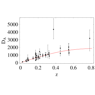
Figure 15: Observational SZE data fitted to our model with the best fit values ${\widehat{H}}_{0}=0.97^{+0.04}_{-0.03}$, $\alpha_{1}=3.2^{+0.1}_{-0.1}$, and $h=0.75\pm 0.05$

.

3.3 Gamma-Ray Burst Hubble Diagram

Gamma-ray bursts (GRBs) are bright explosions visible across most of the Universe, certainly out to redshifts of $z=4.5$ and likely out to $z\sim 10$. Recent studies have pointed out that GRBs may be used as standard cosmological candles. The prompt energy released during burst spans nearly three orders of magnitude, and the distribution of the opening angles of the emission, as deduced from the timing of the achromatic steepening of the afterglow emission, spans a similar wide range of values. However, when the apparently isotropic energy release and the conic opening of the emission are combined to infer the intrinsic, true energy release, the resulting distribution does not widen, as is expected for uncorrelated data, but shrinks to a very well determined value (Frail & Kulkarni (2003)), with a remarkably small (one–sided) scattering, corresponding to about a factor of $2$ in total energy. Similar studies in the X–ray band have reproduced the same results. It is thus very tempting to study to what extent this property of GRBs makes them suitable cosmological standard candles. Schaefer (Schaefer (2003)) proposed using two well known correlations of the GRBs luminosity (with variability, and with time delay) to the same end, while other exploited the recently reported relationship between the beaming–corrected $\gamma$-ray energy and the locally observed peak energy of GRBs (see for instance Dai & al. (2004)). As for the possible variation of ambient density from burst to burst, which may widen the distribution of bursts energies, Frail & Kulkarni (Frail & Kulkarni (2003)) remarked that this spread is already contained in their data sample, and yet the distribution of energy released is still very narrow. There are at least two reasons why GRBs are better than type Ia supernovae as cosmological candles. On the one hand, GRBs are easy to find and locate: even 1980s technology allowed BATSE to locate $\sim$1 GRB per day, despite an incompleteness of about $1/3$, making the build–up of a 300–object database a one–year enterprise. The Swift satellite launched on 20 November 2004, is expected to detect GRBs at about the same rate as BATSE, but with a nearly perfect capacity for identifying their redshifts simultaneously with the afterglow observations . Second, GRBs have been detected out to very high redshifts: even the current sample of about 40 objects contains several events with $z>3$, with one (GRB 000131) at $z=4.5$. This should be contrasted with the difficulty of locating SN at $z>1$, and the absolute lack of any SN with $z>2$. On the other hand, the distribution of luminosities of SNIa is narrower than the distribution of energy released by GRBs, corresponding to a magnitude dispersion $\sigma_{M}=0.18$ rather than $\sigma_{M}=0.75$. Thus GRBs may provide a complementary standard candle, out to distances which cannot be probed by SNIa, their major limitation being the larger intrinsic scatter of the energy released, as compared to the small scatter in peak luminosities of SNIa. There currently exists enough information to calibrate luminosity distances and independent redshifts for nine bursts (Schaefer (2003)). These bursts were all detected by BATSE with redshifts measured from optical spectra of either the afterglow or the host galaxy. The highly unusual GRB980425 (associated with supernova SN1998bw) is not included because it is likely to be qualitatively different from the classical GRBs. Bursts with red shifts that were not recorded by BATSE cannot yet have their observed parameters converted to energies and fluxes that are comparable with BATSE data. We perform our analysis using the data shown in Fig. (16) with the distance modulus $\mu$, given by Eq. (39).

Figure 16: Hubble diagram for the BATSE gamma ray bursts (Schaefer (2003)) up to $z=4.5$.

To this aim, the only difference with respect to the SNIa is that we slightly modify the correction term of Eq. (38), into

$$\Delta m_{G_{eff}}=2.5\gamma\frac{\Delta G_{eff}(t)}{\left(\ln 10\right)G_{eff}}.$$ (57)

We expect that $\gamma$ is of order unity, so that the $G$-correction would be roughly half a magnitude. We obtain $\chi_{red}^{2}=1.09$, and the best fit value is ${\widehat{H}}_{0}=1^{+0.05}_{-0.04}$, $\alpha_{1}=2.8^{+0.1}_{-0.2}$, and $h=0.66\pm 0.05$, which are compatible with the SNIa results. We also confirm that $\gamma=1.5$ as in Eq. (38). In Fig. (18) we compare the best fit curve with both the GRBs and the SNIa Gold Sample.

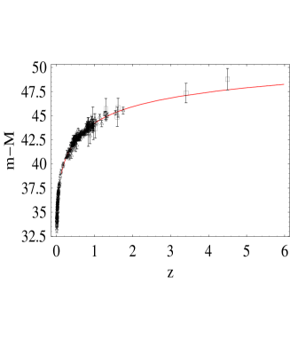
Figure 17: Observational Hubble diagram for the SNIa Gold Sample (Riess et al. 2004), the SNLS data(Astier & al. (2005)) (filled boxes), and the BATSE GRBs data (Schaefer (2003)) (empty boxes) fitted to our model. The solid curve is the best fit curve with ${\widehat{H}}_{0}=1^{+0.05}_{-0.04}$, $\alpha_{1}=2.8^{+0.1}_{-0.2}$, and $h=0.68\pm 0.05$.

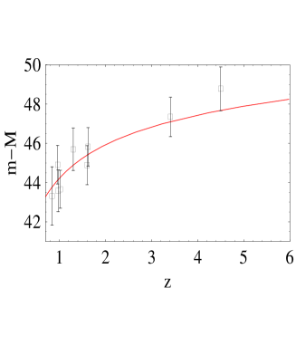
Figure 18: The same as in the Eq. (18) , but zooming on the high redshift GRBs.

3.4 The gas fraction in clusters

In this section we consider a recently proposed test based on the gas mass fraction in galaxy clusters (Allen & al. (2002)). Both theoretical arguments and numerical simulations predict that the baryonic mass fraction in the largest relaxed galaxy clusters should not depend on the redshift, and should provide an estimate of the cosmological baryonic density parameter $\Omega_{b}$ (Eke & al. (1998)). The baryonic content in galaxy clusters is dominated by the hot X - ray emitting intra-cluster gas so that what is actually measured is the gas mass fraction $f_{gas}$ and it is this quantity that should not depend on the redshift. Moreover, it is expected that the baryonic mass fraction in clusters equals the universal ratio $\Omega_{b}/\Omega_{M}$ so that $f_{gas}$ should indeed be given by $b{\times}(\Omega_{b}/\Omega_{M})$, where $\Omega_{M}$ is the matter density parameter, and the multiplicative factor $b$ is motivated by simulations that suggest that the gas fraction is lower than the universal ratio because of processes that convert part of the gas into stars or eject it out of the cluster altogether. Following the procedure described in (Allen & al. (2002, 2004)), we adopt the SCDM model (i.e., a flat universe with $\Omega_{M}=1$ and $h=0.5$, where $h$ is the Hubble constant in units of $100\ {\rm km\ s^{-1}\ Mpc^{-1}}$) as a reference cosmology in making the measurements so that the theoretical expectation for the apparent variation of $f_{gas}$ with the redshift is:

$$f_{gas}(z)=\frac{b\Omega_{b}}{(1+0.19\sqrt{h})\Omega_{M}}\left[\frac{D_{A}^{SCDM}(z)}{D_{A}^{mod}(z)}\right]^{1.5}\,,$$ (58)

where $D_{A}^{SCDM}$ and $D_{A}^{mod}$ is the angular diameter distance for the SCDM and our model respectively. Allen & al. (Allen & al. (2002)) have extensively analyzed the set of simulations in (Eke & al. (1998)) to get $b=0.824{\pm}0.089$, so in our analysis below, we set $b=0.824$. Actually, we have checked that, for values in the $2\sigma$ range quoted above, the main results do not depend on $b$, as also on $\alpha_{3}$. Moreover we have defined the following merit function :

$$\chi^{2}=\chi_{gas}^{2}+\left(\frac{\Omega_{\rm b}h^{2}-0.0214}{0.0020}\right)^{2}+\left(\frac{h-0.72}{0.08}\right)^{2}+\left(\frac{b-0.824}{0.089}\right)^{2}\,,$$ (59)

where we substitute the appropriate expression of $\Omega_{M}$ for our model

$$\chi_{gas}^{2}=\sum_{i=1}^{N_{gas}}{\left[\frac{f_{gas}(z_{i},\alpha_{1},{\widehat{H}}_{0})-f_{gas}^{obs}(z_{i})}{\sigma_{gi}}\right]^{2}}.$$ (60)

Here $f_{gas}^{obs}(z_{i})$ is the measured gas fraction in galaxy clusters at redshift $z_{i}$ with an error $\sigma_{gi}$ and the sum is over the $N_{gas}$ clusters considered. Before presenting results of our analysis it is worth noting that, in order to estimate the gas fraction, it is necessary to evaluate the total cluster mass given by $M_{tot}\equiv{M_{gas}\over f_{gas}}$. Generally the standard assumption used to derive clusters masses from X-ray data is that the system is in hydrostatic equilibrium. This allows one to obtain a mass estimator just through the gas dynamical equilibrium equation:

$$M(<r) = -{rk_{B}T\over G\mu m_{p}}\left[{d\rho_{gas}\over d\ln r}\right]\,,$$ (61)

where $k_{B}$ is the Boltzmann constant, $T$ the cluster gas temperature, $\mu$ the mean molecular weight, $m_{p}$ the proton mass, and $\rho_{gas}$ the gas mass density profile. Let us note that recently Allen & al. (Allen & al. (2004)) have released a catalog of 26 large relaxed clusters with a precise measurement of both the gas mass fraction $f_{gas}$ and the redshift $z$. Actually to avoid possible systematic errors in the $f_{gas}$ measurement, it is desirable that the cluster is both highly luminous (so that the S/N ratio is high) and relaxed, so that both merging processes and cooling flows are absent. We use these data to perform our likelihood analysis, getting $\chi^{2}=1.17$ for 26 data points, and $\alpha_{1}=2.5^{+0.4}_{-0.1}$, ${\widehat{H}}_{0}=0.98\pm 0.04$, $h=0.72\pm 0.05$, and $w_{\phi}=-0.82\pm 0.1$. To complete our analysis we carry out a brief comparison of our results with similar recent results of Lima et al. (Lima & al. (2003)), where the equation of state characterizing the dark energy component is constrained by using galaxy cluster x-ray data. In their analysis, however, they consider quintessence models in standard gravity theories, with a non evolving equation of state, but they allow the so-called phantom dark energy with $w<-1$, what violates the null energy condition. As best fit value of $w$ to the data of (Allen & al. (2002)) they obtain $w=-1.29_{-0.792}^{+0.686}$. In order to directly compare this result with our analysis we first fit the model considered in (Lima & al. (2003)) to the updated and wider dataset of (Allen & al. (2004)), used in our analysis. To this aim we also refer to the model function $f_{gas}(z)$, and the merit function $\chi^{2}$, defined in the Eqs. (58, and 59) respectively. We get $\chi^{2}=1.175$ for 26 data points, and $\Omega_{M}=0.23^{+0.05}_{-0.03}$, $h=0.76^{+0.04}_{-0.09}$, and $w=-1.11\pm 0.35$, so $w<-1$, what corresponds to a phantom energy. We note that our model, instead, gives $w_{\phi}=-0.82\pm 0.1$, what does not violate the null energy condition.  In Fig. (19) we compare the best fit curves for our and the Lima & al. model with the observational data.

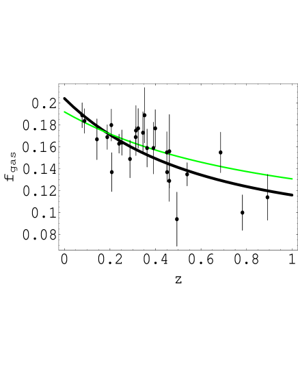
Figure 19: In the diagram we plot the best fit curve to the $f_{gas}$ data for our nmc model (green thin line) and for the quintessence model (black thick line) considered in (Lima & al. (2003)). It is interesting to note the different behaviour of the two curves, even if the statistical significance of the best fit procedure for these two models is comparable: the best fit relative to our nmc model seems to be dominated by smaller redshift data, while the one relative to the Lima & al. model by higher redshift data.

4 Growth of density perturbations

In this section we consider the behavior of scalar density perturbations in the longitudinal gauge $ds^{2}=-(1+2\Phi)dt^{2}+a^{2}(1-2\Phi)d{\bf x}^{2}$. Actually, while in the framework of the minimally coupled theory we have to deal with a fully relativistic component, which becomes homogeneous on scales smaller than the horizon, so that standard quintessence cannot cluster on such scales. In the non minimally coupled quintessence theories it is possible to separate a pure gravitational term both in the stress-energy tensor $T_{\mu\nu}$, and in the energy density $\rho_{\phi}$ , so the situation changes, and it is necessary to consider also fluctuations of the scalar field. However, it turns out (Boisseau & al. 2000 ; Riazuelo & Uzan (2002)) that the equation for dustlike matter density perturbations inside the horizon can be written as follows:

$${\ddot{\delta}_{m}}+2H{\dot{\delta}_{m}}-{1\over 2}G_{\rm Cav}\,\rho_{m}\leavevmode\nobreak\ \delta_{m}\simeq 0\leavevmode\nobreak\ ,$$ (62)

with $G_{\rm Cav}$ is the effective gravitational constant between two test masses and is defined by

$$G_{\rm Cav}={1\over F}\left({2F+4(dF/d\phi)^{2}\over 2F+3(dF/d\phi)^{2}}\right)\leavevmode\nobreak\ .$$ (63)

The equation (62) describes in the non minimally coupled models evolution of the CDM density contrast, $\delta_{m}\equiv\delta\rho_{m}/\rho_{m}$, for perturbations inside the horizon. In our model the Eq.(62) is rather complicated and takes the form

$${\ddot{\delta}_{m}}+\frac{2\left(2\alpha_{2}+\alpha_{1}\left(-\alpha_{3}e^{\alpha_{1}t}-\alpha_{2}t+1\right)\right)}{3\left(\alpha_{3}+e^{\alpha_{1}t}+\alpha_{2}t-1\right)}{\dot{\delta}_{m}}+$$

$$-\frac{e^{\alpha_{1}}\left(\alpha_{1}\alpha_{2}+e^{\alpha_{1}}\left(\alpha_{1}^{2}-16V_{0}\right)\right)}{6\left(\alpha_{2}+e^{\alpha_{1}}+\alpha_{3}-1\right)^{2}\left(\alpha_{3}+e^{\alpha_{1}t}+\alpha_{2}t-1\right)a_{i}^{3}}\delta_{m}=0,$$

where

$$\alpha_{2}=\displaystyle\frac{\alpha_{1}\left(-\alpha_{3}+e^{\alpha_{1}}+1\right)-3{\widehat{H}}_{0}\left(\alpha_{1}+e^{\alpha_{1}}-1\right)}{3{\widehat{H}}_{0}+\alpha_{1}-2}.$$ (65)

The Eq. (4) does not admit exact solutions, and can be solved only numerically. However, since with our choice of normalization the whole history of the Universe is confined to the range $t\in[0,1]$ and therefore to study the behavior of the solution for $t\simeq 0$ we can expand the exponential functions in Eq. (4) in series around $t=0$. We obtain an integrable Fuchsian differential equation, which is a hypergeometric equation. We then use the obtained exact solution to set the initial conditions at $t=0$ to numerically integrate Eq. (4) in the whole range $[0,1]$. We use the growing mode $\delta_{+}$ to construct the growth index $f$ as

$$f\equiv\frac{d\ln\delta_{+}}{d\ln a}\,,$$ (66)

where $a$ is the scale factor. Once we know how the growth index $f$ evolves with redshift and how it depends on our model parameters, we can use the available observational data to estimate the values of such parameters, and the present value of $\Omega_{{\rm M0}}$. The 2dFGRS team has recently collected positions and redshifts of about $220000$ galaxies and presented a detailed analysis of the two-point correlation function. They measured the redshift distortion parameter $\beta=\displaystyle{f\over b}$, where $b$ is the bias parameter describing the difference in the distribution of galaxies and mass, and obtained that $\beta_{|z\rightarrow 0.15}=0.49\pm 0.09$ and $b=1.04\pm 0.11$. From the observationally determined $\beta$ and $b$ it is now straightforward to get the value of the growth index at $z=0.15$ corresponding to the effective depth of the survey. Verde & al. (Verde & al. (2001)) used the bispectrum of 2dFGRS galaxies, and Lahav & al.  (Lahav & al. (2002)) combined the 2dFGRS data with CMB data, and they obtained

$$b_{verde} = 1.04\pm 0.11\,,$$ (67)

$$b_{lahav} = 1.19\pm 0.09\,.$$ (68)

Using these two values for $b$ we calculated the value of the growth index $f$ at $z=0.15$, we get respectively

$$f_{1} = 0.51\pm 0.1\,,$$ (69)

$$f_{2} = 0.58\pm 0.11\,.$$ (70)

To evaluate the growth index at $z=0.15$ we first have to invert the $z-t$ relation and find $t_{0.15}$. Then, substituting $z=0.15$ and the two values of $f_{1}$ and $f_{2}$ we calculate ${\widehat{H}}_{0}$ and $\alpha_{1}$. Actually the $z-t$ relation is rather involved and cannot be exactly inverted, so we apply this procedure numerically. We get $\alpha_{1}=3.3\pm 0.05$, ${\widehat{H}}_{0}=0.98^{+0.05}_{-0.02}$,   $V_{0}=0.5\pm 0.06$ which corresponds to $\Omega_{\Lambda_{0}}=0.65\pm 0.08$. In Fig. (20) we show how the growth index is changing with redshift in our non minimally coupled model as compared with a standard quintessence model namely the minimally coupled exponential model described in (Demianski & al. (2005)). We note that at low redshift theoretical predictions of these different models are not distinguishable, independent measurements from large redshift surveys at different depths can disentangle this degeneracy.

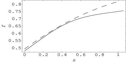
Figure 20: The growth index $f$ in different cosmological models: the solid line corresponds to our non minimally coupled model. The dashed curves correspond to a more standard quintessence model with an exponential potential (described in Demianski & al. (2005)).

5 Conclusions

In this paper we have shown that in the framework of non minimally coupled scalar tensor theory of gravitation it is possible to consider homogeneous and isotropic cosmological models with time dependent dark energy component. These models have a very interesting feature of producing in a natural way an epoch of accelerated expansion. In these models initially the over all density of the universe is dominated by matter (for the sake of simplicity we do not include radiation into our consideration) and later on the energy density of the scalar field becomes dominant and the universe enters an accelerated phase of its evolution. It turns out that at large $t$ asymptotically $w_{\phi}\rightarrow-1$, and such a transition to the asymptotical value is responsible for the accelerated expansion. The equation of state can admit a superquintessence behavior ($w<-1$), without violating the weak energy condition, just as an effect of the transition toward $w\rightarrow-1$. The energy density of the scalar field decreases with time but before the present epoch it starts to dominate the expansion rate of the universe and asymptotically for $t\rightarrow\infty$ the universe is reaching a de Sitter stage. To check viability of our model we have compared its predictions with the available observational data and it turned out that with an appropriate choice of parameters our model is reproducing the observed characteristics of the universe. Let us note that since in order to exactly solve the dynamical equations we have not included radiation into our consideration we do not use CMB data and observed abundances of light elements in confrontation of theoretical predictions of our model with observational data.

In Tab.(1) we present results of our analysis, they show that predictions of our model are fully compatible with the recent observational data.

Table 1: The basic cosmological parameters derived from our model are compared with observational data.

$\mathbf{\alpha_{1}}$	$\mathbf{{\widehat{H}}_{0}}$	$\mathbf{\Omega_{\Lambda_{0}}}$	w	dataset
$2.9^{+0.3}_{-0.2}$	$1.0^{+0.03}_{-0.04}$	$0.84^{+0.06}_{-0.07}$	$-0.86\pm 0.06$	Gold SNIa + SNLS
$3.2^{+0.1}_{-0.09}$	$0.97^{+0.04}_{-0.07}$	$0.62\pm 0.08$	$-1.1\pm 0.15$	SZe
$2.5^{+0.3}_{-0.2}$	$1^{+0.05}_{-0.03}$	$0.8\pm 0.15$	$-0.76\pm 0.1$	dimensionless coordinate
$2.8^{+0.1}_{-0.2}$	$1^{+0.05}_{-0.04}$	$0.84\pm 0.05$	$-0.81\pm 0.07$	GRBs
$2.5^{+0.4}_{-0.1}$	$0.98\pm 0.04$	$0.76\pm 0.06$	$-0.82\pm 0.1$	gas fraction in clusters
$3.3\pm 0.05$	$0.98^{+0.05}_{-0.02}$	$0.65\pm 0.08$	$-1.1\pm 0.07$	galaxies peculiar velocity
$\mathbf{3.2\pm 0.04}$	$\mathbf{0.99\pm+0.02}$	$\mathbf{0.77\pm 0.03}$	$\mathbf{-0.9\pm 0.04}$	averaged mean

6 Appendix I

As was already noted the solution of the coupled system of the Einstein equations and generalized Klein-Gordon equation describing our model can be written in the form

$$a(t)=A(s)\left(B(s)t^{3\over{s+3}}+{D\over{\Sigma_{0}}}\right)^{{s+1}\over s}t^{{2s^{2}+6s+3}\over{s(s+3)}}\,,$$ (71)

$$\phi(t)=C(s)\left(-{V_{0}\over\gamma(s)}B(s)t^{3\over{s+3}}+{D\over\Sigma_{0}}\right)^{-{{2s+3}\over 2s}}t^{-{(2s+3)^{2}\over{2s(s+3)}}}-\phi_{0}\,,$$ (72)

where $A(s)$, $B(s)$, $C(s)$, $\gamma(s)$ and $\chi(s)$ are given by

$$A(s) = \left({\chi(s)}\right)^{s+1\over s}\left({(s+3)\Sigma\over 3\gamma(s)}\right)^{s+2\over s+3}\,,$$ (73)

$$B(s) = \left({(s+3)\Sigma\over 3\gamma(s)}\right)^{-{3\over(s+3)}}{(s+3)^{2}\over s+6}\,,$$ (74)

$$C(s) = \left({\chi(s)}\right)^{-{(2s+3)\over 2s}}\left({(s+3)\Sigma\over 3\gamma(s)}\right)^{-{(3+2s)\over 2(s+3)}},$$ (75)

and

$$\gamma(s) = {2s+3\over 12(s+1)(s+2)}\,,$$ (76)

$$\chi(s) = -{2s\over 2s+3}\,.$$ (77)

References

- Allen & al. (2002) Allen S.W., Schmidt R.W., Fabian A.C., 2002, MNRAS, 334, L11
- Allen & al. (2004) Allen S.W., & al. 2004, MNRAS, 335, 457
- Astier & al. (2005) Astier P., & al., 2006, A&A, 447, 31
- (4) Boisseau B., Esposito-Farese G., Polarski D., Starobinsky A.A., 2000, Phys. Rev. Lett., 85, 2236
- Birkinshaw (1999) M. Birkinshaw, 1999, Phys. Rep., 310, 97
- Caldwell, Dave & Steinhardt (1998) Caldwell R.R., Dave R., Steinhardt P.J., 1998, Phys. Rev. Lett., 80, 1582
- Capozziello & al. (1996) Capozziello S., de Ritis R., Rubano C., and Scudellaro P., Riv. del Nuovo Cimento, 19, vol. 4 (1996).
- (8) Cavaliere A., Fusco–Femiano R., 1976, A&A, 49, 137; Cavaliere A., Fusco–Femiano R., 1978, A&A, 70, 677
- Dai & al. (2004) Dai Z. G., Liang E. W. & Xu D. 2004, ApJ, 612, L101
- Daly & Djorgovski (2004) Daly R.A., Djorgovski S.G. 2004, ApJ, 612, 652
- Demianski & al. (2003) Demianski M., de Ritis R., Marino A.A., Piediaplumbo E., 2003, A&A, 411, 33
- Demianski & al. (2005) Demianski M., Piedipalumbo E., Rubano C., Tortora C., 2005, A&A, 431, 27
- Eke & al. (1998) Eke V., Navarro J.F., Frenk C.S., 1998, ApJ, 503, 569, 1998
- Frail & Kulkarni (2003) Frail D. A. & Kulkarni S. R. 2003, ApJ, 594 674
- (15) Gaztañaga E., Garcia-Berro E., Isern J., Bravo E., & Dominguez, 2002, Phys. Rev., D65, 023506
- Lahav & al. (2002) Lahav O., Bridle S. L., Percival W. J., & the 2dFGRS Team, 2002, MNRAS, 333, 961
- Lima & al. (2003) Lima J. A. S., Cunha J. V., & Alcaniz J. S., 2003, Phys. Rev., D68, 023510
- Peebles & Ratra (1988) Peebles P.J.E. and Ratra B., 1988, Astrophys. J., 325, L17
- Perrotta, Baccigalupi & Matarrese (2000) Perrotta F., Baccigalupi C., and Matarrese S., 2000, Phys.Rev., D61, 023507
- Reese & al. (2002) Reese E. et al., 2002, ApJ, 581, 53
- Riazuelo & Uzan (2002) Riazuelo A., & Uzan J.- P., 2002, Phys. Rev., D66, 023525
- Riess & al. (1998) Riess A.G., et al., 1998, AJ, 116, 1009
- Riess (2000) Riess A.G., 2000, PASP, 112, 1284
- Riess & al. (2004) Riess A.G., Strolger L.-G., Tonry J., & al., 2004, ApJ, 607, 665
- Sarazin (1988) C.L. Sarazin, “X-Ray Emission from Cluster of Galaxies”, Cambridge Univ. Press, Cambridge (1988).
- Schaefer (2003) Schaefer B.E., ApJ, 2003, 583, L67
- Schmidt & al. (1998) Schmidt B. P., Suntzeff N. B., Phillips M. M, & al., 1998, ApJ, 507, 46
- Spergel & al. (2003) Spergel D.N., Verde, L., Peiris H. V, & al., 2003, ApJ, 148, 175
- (29) Steinhardt P.J., Wang L., and Zlatev I., 1999, Phys. Rev., D59, 123504
- Tonry et al. (2001) Tonry J. L., et al., 2003, ApJ, 594, 1
- Weinberg (1989) Weinberg S., 1989, Rev. Mod. Phys., 61, 1
- Urena-Lopez & Matos (2000) Urena-Lopez L.A. and Matos T., 2000, Phys. Rev., D62, 081302
- Uzan (2003) Uzan J.Ph., Rev. Mod. Phys., 2003, 75, 403
- Verde & al. (2001) Verde L., Kamionkowski M., Mohr J. J., Benson A.J., 2001, MNRAS, 321, L7
- Zeldovich (1967) Zeldovich Ya. B., 1967, Pis’ma Zh. Eksp. Teor. Fiz., 6, 883; (1967, JETP Lett., 6, 316 ).
- Zlatev, Wang & Steinhardt (1999) Zlatev I., Wang L., and Steinhardt P.J., 1999, Phys. Rev. Lett., 82, 896