An analysis method for time ordered data processing of Dark Matter experiments

Abstract

Context. The analysis of the time ordered data of Dark Matter experiments is becoming more and more challenging with the increase of sensitivity in the ongoing and forthcoming projects. Combined with the well-known level of background events, this leads to a rather high level of pile-up in the data. Ionization, scintillation as well as bolometric signals present common features in their acquisition timeline: low frequency baselines, random gaussian noise, parasitic noise and signal characterized by well-defined peaks. In particular, in the case of long-lasting signals such as bolometric ones, the pile-up of events may lead to an inaccurate reconstruction of the physical signal (misidentification as well as fake events).

Aims. We present a general method to detect and extract signals in noisy data with a high pile-up rate and qe show that events from few keV to hundreds of keV can be reconstructed in time ordered data presenting a high pile-up rate.

Methods. This method is based on an iterative detection and fitting procedure combined with prior wavelet-based denoising of the data and baseline subtraction.

Results. We have tested this method on simulated data of the MACHe3 prototype experiment and shown that the iterative fitting procedure allows us to recover the lowest energy events, of the order of a few keV, in the presence of background signals from a few to hundreds of keV. Finally we applied this method to the recent MACHe3 data to successfully measure the spectrum of conversion electrons from ${}^{57}{\rm{Co}}$ source and also the spectrum of the background cosmic muons.

1 Introduction

Evidence for the existence of non-baryonic Dark Matter seems to be well established from the results of recent cosmological observations : CMB anisotropy measurements Spergel et al. (2003); Benoit et al. (2003); Rebolo et al. (2004); MacTavish et al. (2005), large scale structure surveys Tegmark et al. (2004) and type Ia supernova measurements Perlmutter et al. (1999). The leading candidate intended to composed non-baryonic dark matter, is the lightest neutralino $\tilde{\chi}$ proposed by supersymmetric extensions of the standard model of Particle Physics Jungman et al. (1996). A great amount of non-baryonic Dark Matter detectors Akerib et al. (2005); Angloher et al. (2005); Sanglard et al. (2005) have been developed using different and complementary techniques to access to the energy release. The related signals which are measured, can be ionization, scintillation or heat released by the particle interaction. The simultaneous measurement of a combination of at least two of the latter quantities are used in order to achieve a high rejection factor against background events and systematic effects.

${}^{3}{\mathrm{He}}$ has been proposed as a sensitive medium Mayet et al. (2000); Santos et al. (2000) to overcome well-known limitations of existing Dark Matter detectors, such as for example the discrimination between WIMPs and background neutrons. Moreover such a nucleus will be sensitive to the axial interaction of the neutralino $\tilde{\chi}$, making a ${}^{3}{\mathrm{He}}$-based detector complementary to most of existing detectors Mayet et al. (2002); Moulin et al. 2005a .
Following early works Pickett (1988); Bunkov et al. (1995); Bauerle et al. (1998) on a ${}^{3}{\mathrm{He}}$ superfluid cell at ultra low temperature $\rm\sim 100\mu K$, a 3-cell prototype, MACHe3 (MAtrix of Cells of ${}^{3}{\mathrm{He}}$), has been developed. It has been used to demonstrate for the first time the possibility to measure events in the keV energy range in ${}^{3}{\mathrm{He}}$ Moulin et al. 2005b .

As for many other bolometric detectors, e.g. Edelweiss Sanglard et al. (2005), Archeops Tristram et al. (2005); Macías-Pérez et al. (2005), the raw data of MACHe3 consist of time ordered samples with four main components : 1) A baseline coming mainly from low frequency fluctuations of the thermal bath used to cool down the detector. 2) Random Gaussian noise. 3) Parasitic noise characterized by medium and high frequency structures. 4) The signal of interest convoluted by the bolometer time response. The latter when related to the energy deposited by incoming particles leads to peaks in the data. In this paper we present the method developed for the analysis of these data Moulin et al. 2005c . In particular we focus on the detection of peaks in noisy data presenting a high level of pile-up. The method and algorithms used for this analysis are general and may well be used for other applications.

This paper is organized as follows. Section 2 presents the main characteristic of typical bolometric data. In section 3 we deal with the details of the processing procedure. Sections 4 and 5 presents the main results obtained after processing of the simulated and of the MACHe3 data respectively. Finally, we conclude in section 6.

2 Description of the time ordered data

We present in this section the main characteristics of the MACHe3 experiment and of its raw time ordered data which as described above are shared by other bolometric detectors.

2.1 Experimental set-up

A multi-cell prototype of MACHe3, with three bolometer cells (A, B and C) aligned longitudinally, has been developed and operated at the nominal temperature of $\rm 100\ \mu K$ Moulin et al. 2005b . The time constant for thermal relaxation of the cell is of the order of $\rm 3\ s$ Each cell contains one vibrating wire resonator which is used to measure the energy released Bauerle et al. (1998); Triqueneaux et al. (1999).

A ${}^{57}{\rm{Co}}$ radioactive source, which provides low energy electrons, was spot-welded in the inner wall of the center cell (B). Because of the short free path of electrons in ${}^{3}{\mathrm{He}}$, $\rm\leq 370\ \mu m$ for an energy below $\rm 40\ keV$, the energy released by the interacting electrons will be fully detected within that cell. Further because of the relatively high activity of the source, for Dark Matter concern, about 0.06 Bq, we expect conversion electrons to pile-up at the experiment sampling rate of 100 ms. In addition to electrons, events corresponding to cosmic muons and $\gamma$-rays of 14.4, 122 and 136 keV emitted by the source are expected in the three cells.

2.2 Example of raw data at 100 $\mu$K 

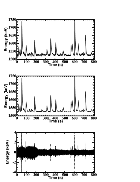
Figure 1: Top: raw data from the central cell of the MACHe3 prototype, corresponding to the energy released (in $\rm keV$) as a function of time. Events are coming from cosmic muons and low energy conversion electrons from a $\rm{}^{57}Co$ source spot-welded on the inner wall of the cell. Microvibrations as well as statistical noise add up to the baseline fluctuations. The sampling rate is 100 ms. Middle: same data but after applying the denoising algorithm. Bottom: Residuals between raw and denoised data on an expanded scale. See text for details.

The raw data consists of a sequence of peaks corresponding to the energy released by interacting particles inside the cell. The peaks are characterized by a rising and a relaxing time. The first one is related to the quality factor of the wire (Q$\sim$10⁴) whereas the second depends on the geometry of the cell and the size of the orifice. The upper plot on figure 1 shows a typical acquisition spectrum with $\rm 100\ ms$ sampling rate from the cell containing the ${}^{57}{\rm{Co}}$ source (B cell). We can observe a baseline in data corresponding to low frequency fluctuations of the thermal bath. Cosmic muons as well as very low energy events corresponding to electrons coming from the source are visible. Given the relatively high activity of ${}^{57}{\rm{Co}}$ source we observe a high level of pile-up in the data corresponding to multiple electron events, Auger as well as conversion, and also to combinations of muons and electrons. The pile-up needs to be carefully treated in the analysis for an accurate reconstruction of the low energy events.

Notice that peaks in the data whatever their origin (muons, $\gamma$-rays, electrons) are identical in shape (same characteristic time constants). This is why, for the purpose of the analysis, we will define in the following a reference peak with only one free parameter: the amplitude which is given by the amount of energy released inside the cell.

3 Data analysis method

We have developed an analysis method in four main steps. First of all, we reduce significantly the statistical noise in the data using a denoising algorithm. Second, the low frequency baseline in the data is removed as estimated from the local minima. Then, we estimate the shape of the bolometer time response by extracting a reference peak from the data. Finally, we apply to the data an iterative fitting procedure taking as model the reference peak.

3.1 Data denoising

The time ordered data are processed in pieces each consisting of 8192 samples. To reduce the statistical noise, a wavelet-based denoising method is applied to data. This procedure is based on a shrinkage algorithm with conditional means as described by Percival et al. (2000). It presents two free parameters $j_{max}$ and $p$ :

• $j_{max}$ is related to the maximal wavelet scale at which the denoising is applied. This implies that data are not modified at higher scales. This parameter is chosen to keep both the shape and the amplitude of the peaks and reduce significantly the noise. In other words, we focus in the high frequency noise and we do not modify the low frequency components in the data.

• $p$ expresses the quality required for the denoising and is fixed to 0.9 for our analysis. This value was chosen empirically but in general for values between 0.8 and 0.95 the results present not significant differences.

In the middle plot of figure 1 we present the data after applying the denoising algorithm. We can observe that the method allows us to preserve both the shape and amplitude of the events. This is indicated by the residuals between raw and denoised data plotted on the bottom on an expanded scale. Residual amplitudes are about 1 keV or less. Shapes of the peaks are unchanged. Typically for a 200 keV peak, the residual is at most of the order of 4 keV.

3.2 Baseline subtraction

We clearly observe in the bolometric time ordered data a baseline related to the low frequency drifts of the thermal bath temperature plus a constant value. Due to the high level of pile-up in the data, the determination and subtraction of this baseline is difficult. An standard direct fit of this baseline is highly biased by the presence of the signal peaks and the baseline is poorly reconstructed. In the same way, the application of another standard technique based on the localization and subtraction of the peaks reduces too much the data to which the fitting procedure can be applied.
After careful analysis of the properties of this baseline, we realized that it can be defined by the local minima in the data as the peaks from particle interactions do not contribute to these minima. We assume that the noise distribution is double-tailed and the peak signal strictly positive. In practice, we search for local minima in intervals of 812 samples making a total of 10 minima in the 8192 channel sample. The identified minima computed in this way are then fitted to a polynomial. We have found that in 8192 channel sample, a first order polynomial reproduces very well the baseline, as temperature fluctuations of the ${}^{3}{\mathrm{He}}$  bath are at very low frequency. The polynomial fit is then subtracted from the data preserving both the shape and the amplitude of the peaks.

3.3 Reference peak

As pointed out previously, a particle interaction produces a peak characterized by a rising and decreasing time (see section 1) which depends only on the instrumental set up and does not depend on the amplitude of the signal as long as the detector does not saturate. Because of this, it is useful to define a normalized reference peak (with an amplitude of 1) which will mimic the shape of the peaks observed in the data and which can be used for further analysis of these data (see section 3.4). To mimic at best the signal, we directly select the reference peak from the data with no modeling. The chosen candidate must not be affected by pile-up and must have a high signal to noise (amplitude versus r.m.s. noise) to limit the impact of the noise contribution. In practice, we have chosen an isolated peak with signal to noise ratio larger than 10 which is normalized to an amplitude of unity. To ensure a high quality posterior analysis the peak is then completed from time equal to 8 s, with a decreasing exponential function over a total of 1024 data samples. In this way we account for the high end of the tail of the bolometric time response which is below the noise level for the acquisition data. Figure 2 shows the reference peak extracted from the data and which was used for the data processing presented below.

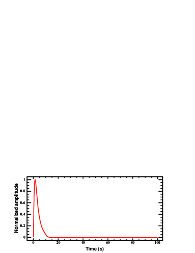
Figure 2: Reference peak for data processing. This peaks was extracted directly from the data (see text for details) and completed from time equal to 8 s, by a decreasing exponential to mimic at best the time response of the bolometer. The sampling rate is 100 ms.

3.4 Iterative fitting procedure

We have developed an iterative fitting procedure to extract the energy released in the bolometric cells by the interacting particles. This procedure is based on three main steps.

1. We search for the peaks on the data and flag them as detected. For this purpose, we compute the first derivative of the data. Then we select, on this new data set, all samples for which the amplitude of the signal is five times larger than the r.m.s noise (i.e. all samples with a signal to noise ratio better than five). This allows us to get intervals in which a peak will be fitted. For a single peak we may flag various samples which in some cases may be unconnected. To avoid fitting multiple peaks when only a single one is detected but still to allow for the detection of piled-up peaks, we broaden the flags over 35 samples. This is about twice the rising time of the bolometer response.

2. We fit to the data as many model-peaks as peaks where flagged in the previous step, with a minimization of the mean square deviation between the data and the fit. The free parameters in the fit are the position and the amplitude of the peak. Each model-peak is constructed from the reference peak with initial position and amplitude given by the position and value of the maximum of the signal within the corresponding flagged peak. It is important to note that the peaks detected at the previous iteration are refitted in the current iteration. It leads to a better fit for these peaks as contributions of other peaks detected during the actual iteration can be taken into account.

3. We subtract the fitted model-peaks from the original data to estimate the residuals on the fitting procedure. If the fit was perfect, the residuals would directly correspond to the noise in the data. Therefore, we can define, for each fitted peak, a signal to noise ratio ($\rm S/N$) by dividing the amplitude of the fitted peak by the maximum of the absolute value of the residuals over 35 samples centered at the position of the maximum. Finally, each fitted peak is flagged and we take these flags and the residuals as inputs for the next iteration step. This way we can search for smaller amplitude peaks keeping a trace of the larger amplitude ones.

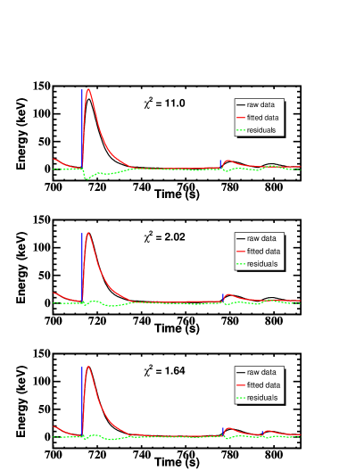
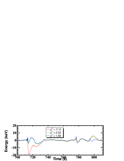
Figure 3: From top to bottom the first three plots present the data (in black), the best fit the data (in red) and the residuals (in green) for consecutive iterations of the algorithm with reduced $\chi^{2}$ values of, $11$, $2.02$ and $1.64$ respectively. Vertical solid lines (in blue) show the position and the amplitude of the fitted peak for each iteration. On the bottom plot, we represent the residuals for the above three iterations in red, green and blue respectively. The amplitude of the signal is given in keV, see Moulin et al. 2005b for details.

These three steps are repeated until no peak at 5$\sigma$ is found in the residual data meaning that we reached the noise level. In general we need about 10 iterations per piece of data. To avoid the algorithm to diverge we stop the iterative procedure when more than 20 iterations are performed and that piece of data is not used for further analysis (less than 1 % of the data). At each iteration the position, the amplitude and the signal to noise ratio are recorded for each detected peak. We characterize the quality of the fit using a $\chi^{2}$ test. The fit to the data with the smallest reduced $\chi^{2}$ is chosen as best fit. Such a procedure allows us to have access to the peaks with the smallest amplitudes, in which we are particularly interested.

As an illustration of the above method, we present in figure 3 the iterative analysis of a sample of raw data corresponding to 110 seconds of acquisition time. From top to bottom the first three plots trace the data (in black), the best fit to the data (in red) and the residuals (in green) for consecutive iterations of the algorithm with reduced $\chi^{2}$ values of $11$, $2.02$ and $1.64$ respectively. On the bottom plot, we represent the residuals for the above three iterations in red, green and blue respectively. We can clearly observe from those figures how the fit improves from one iteration to another. Further, by comparing the second and third plots, we remark that the peak at 800 s is identified by the algorithm only in the third iteration. This is because the residuals at the end of iteration 2 have finally decreased to lower than the amplitude of the 800 s peak. Notice that only iteratively we can achieve such a precision on the fit and therefore recover the lowest amplitude peaks in the data.

4 Application to simulated data

We present in this section the application of the above analysis method to the simulated MACHe3 data. We characterize the quality of the reconstruction of the signal using as parameters both the efficiency of detection and the contamination from spurious detections.

4.1 Simulation of time ordered data

To estimate the efficiency of the analysis method presented in the previous section, we have produced fake time ordered data from physical simulations using the Geant4 package Agostinelli et al. (2003). For these simulations, we fully reproduced the instrumental set-up taking particular care of the detector geometry as well as of the materials and we included the physical processes involved. More precisely, the G4EMLOW2.3 package has been used to perform an adequate and accurate treatment of low energy electromagnetic interactions. As discussed before, the expected events in the data are related to cosmic muons, $\gamma$-rays and electrons from the ⁵⁷Co source. For each contribution, the simulation allows to compute its energy distribution. $\gamma$-rays at $\rm 14.4$, $\rm 122$ and $\rm 136\ keV$ are emitted isotropically from the $\rm{}^{57}Co$ source, assuming an activity of $\rm 0.06\ Bq$. Both conversion and Auger electrons are taken into account. The energy corresponding to each line is weighted to respect its intensity deduced from the decay scheme of the $\rm{}^{57}Co$ source.

The simulated timeline for each cell is obtained as follows. 1) The amplitude of each peak in the timeline is randomly chosen from the simulated energy distribution of the events. Indeed, the rates of each particle is recovered in the simulated time line. 2) These amplitudes are then convolved by the estimated reference peak as shown on Fig. 2. 3) The peaks are uniformly distributed on the timeline so that we can reproduce the pile-up observed in the data. 4) White noise is eventually added to the simulated timeline. The noise as observed in the experimental timeline can be in a first approximation considered as white noise with a dispersion of $\rm 1-2\ keV$. However notice that in here we do not take into account more complex structures in the noise nor parasitics in the data such as microvibrations.

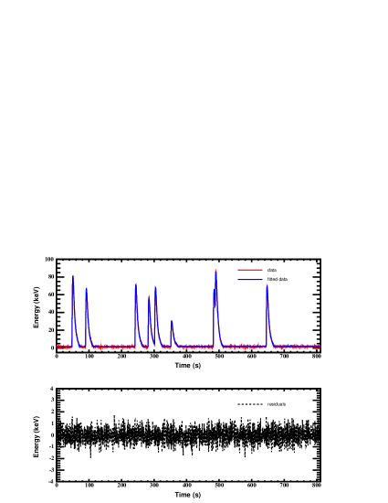
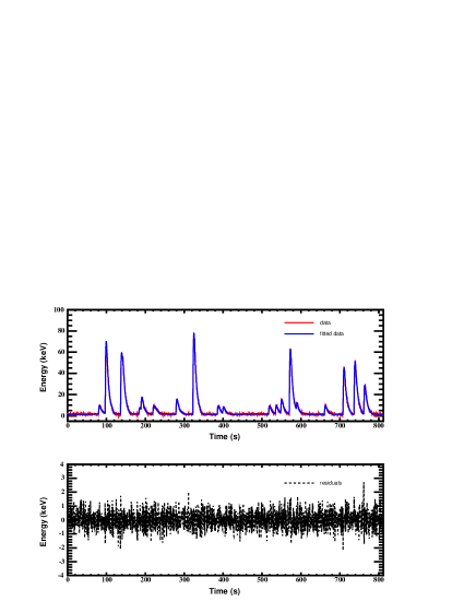
Figure 4: From top to bottom, simulated data sample (red solid line) for A and B set of simulations respectively. The best fit to the simulated data is presented (solid blue line) as well as the residuals (dotted line). Residuals in each case are presented on an expanded scale below (black dashed line).

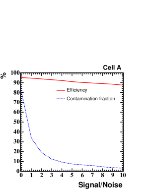
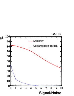
Figure 5: From left to right, global detection efficiency (in red solid line) and contamination fraction (in blue dashed line) as a function of cut in the $\rm S/N$ ratio for the A and B set of simulations respectively (see text for details).

4.2 Reconstruction of the simulated data

As a first step we concentrate in the analysis of a sample of simulated data of about $\rm 819\ s$. Figure 4, from top to bottom, shows in red this data sample after denoising and baseline subtraction for two different sets of simulations A and B respectively. The fit to the data is presented in blue and the lowest figure presents the residuals between data and fitted data. The r.m.s. of the residuals is lower than 1 keV.

In the A simulations we include cosmic muons and $\gamma$-rays to reproduce the features of the MACHe3 A cell. The B simulations include in addition the simulated conversion electrons for ${}^{57}{\rm{Co}}$ source to mimic the data in the MACHe3 B cell. We plot in blue the best fit to the data and in dashed black line the residuals after subtraction of the latter.

In the case of the A simulations, the input timeline consists of 9 events. After analysis we recover 23 peaks among which 9 are considered as detected (meaning S/N $>1$) and 14 as non-detected (meaning $\rm S/N<1$). By imposing this detection condition, we reject all spurious detections. Further, all the detected peaks present high $\rm S/N$ ($\rm\geq 39$) as could be expected since the simulated timeline does only contain large amplitude peaks corresponding to the $\mu$ contributions with a relatively low pile-up rate.

In the case of the B simulations, the input timeline consists of 25 peaks with amplitudes ranging from 5 to 85 keV corresponding to the $\mu$, $\gamma$ and $e^{-}$ contributions). Imposing the simple detection condition, $\rm S/N\geq 1$, 19 peaks are recovered from the best fit timeline and we have no spurious detection. We can therefore consider that the rest of detected peaks represents the noise in the detection. In this particular case, just considering only peaks with $\rm S/N\geq 1$ is enough to remove all the noise contribution. However, in the general case a careful study has to be performed to identify which $\rm S/N$ cut is needed to have a negligible noise contribution.

From these results, we clearly observe that the efficiency of reconstruction of the input signal will depend very much both on the amplitude of the peaks and on the level of pile-up. Therefore, to fully characterize the quality of the method we consider in the following, 1) the efficiency of detection, defined as the number of reconstructed peaks divided by the total number of input peaks, and, 2) the contamination fraction, defined as the number of spurious detections divided by the total number of detected peaks. Both quantities have been calculated as a function of S/N.

4.3 Global analysis of the quality of the method

We have performed a global analysis of the quality of reconstruction of the method based on $\rm 15.5\ h$ of simulated data for the A and B cells. Figure 5 shows from left to right the efficiency of detection, in red, and the contamination fraction, in blue, as a function of the cut in the $\rm S/N$ ratio of the detected peaks for the A and B cells respectively.

For the A set of simulations, we observe that the efficiency of detection is roughly constant with the $\rm S/N$ cut. However the contamination fraction quickly decreases and, in particular, it is under 5 % for $\rm S/N$ cuts of 5 or above.

For the B set of simulations, the efficiency of detection decreases significantly for large values of $\rm S/N$ cut with a turnover between 4 and 5. This is due to the fact that the low amplitude peaks and specially those of a few keV are difficult to fit with a background noise level of about 1 keV but also to the high level of pile-up which reduces the discrimination of the algorithm. With respect to the latter, it can be observed that for some of the pile-up peaks, the best fit to the data indicates more peaks than are really in the data.

From the previous results we can conclude that a $\rm S/N$ cut of 5 would be a good compromise in terms of low contamination fraction and sufficiently high detection efficiency for both the A and B set of simulations. Indeed, the contamination fraction would be less than 5 % for the A simulations and negligible (at the accuracy of our simulations) for the B simulations. The efficiency of detection would be of the order of 90 % for the A simulations and above 60 % for the B simulations. Further, it can be noted that the contamination fraction is higher in the cell A than in cell B due to the smaller number of total detected peaks.

4.4 Evolution of the reconstructed simulated spectrum with the $\rm S/N$ cut

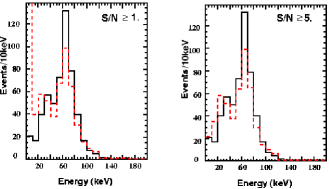
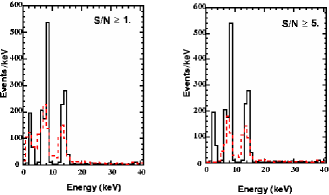
Figure 6: In the top and bottom panels, we plot, in red, the reconstructed simulated spectrum for the A set of simulations in the energy range $[0,200]$ keV and for the B set of simulations in the energy range $[0,40]$ keV for $\rm S/N$ cuts of 1 (left plot) and 5 (right plot). The input spectrum is overplotted in solid black line.

To complete the global picture presented above, we concentrate now in the analysis of the quality of the reconstruction of the input energy spectrum of the signal. For this purpose we show in figure 6, the reconstructed spectrum in red and the input spectrum in black for the A (top panel) and B (bottom panel) simulations for values of the $\rm S/N$ cut of 1 (left plot) and 5 (right plot).

In the case of the A set of simulations, for a $\rm S/N$ cut of 1, the reconstruction is very good for energies above 20 keV but below we clearly observe spurious signals. When assuming a $\rm S/N$ cut of 5 the contribution of the spurious signal is removed significantly at low energies and the quality of the reconstruction is maintained above 20 keV. The differences observed between the reconstructed and the input spectra comes, on one hand, from the fact that the algorithm does not have 100 % efficiency and, on the other hand, by the errors on the determination of the amplitude of peaks which tend to smear out the spectrum.

In the case of the B set of simulations, the analysis is more complex. For energies above 20 keV we recover the same behavior than for the A simulations as the signal is dominated by the cosmic $\mu$ contribution. At energies between 1 and 5 keV, and for a $\rm S/N$ cut of 1 we clearly observe the contribution from spurious signals which is of the same order of that observed for the A simulations. Although a significant contribution from the spurious signal is still present we can clearly distinguish the three energy lines corresponding to electrons of $\rm\sim 2\ keV$ (pile-up of L-shell Auger electrons from ${}^{57}{\rm{Co}}$ ), $\rm 7.3\ keV$ and $\rm 13.6\ keV$ (conversion electrons). For a $\rm S/N$ cut of 5 the spurious signal is roughly completely removed but the electron line at $\rm\sim 2\ keV$ is lost. However, the lines at 7.3 and 13.6 keV are preserved although smeared out in the same way as discussed above for the A simulations.

4.5 Efficiency of the reconstruction for low energy events.

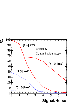
Figure 7: Detection efficiency (red solid line) and contamination fraction (blue dashed line), in the energy ranges 1-5 keV and 5-10 keV as function of $\rm S/N$ cut for the B set of simulations.

In the analysis of the B cell data presented in the following section we are particular interested in the reconstruction of the very low amplitude events in the energy range from 1 to 16 keV (range of energies for conversion electrons). As discussed above for our choice of $\rm S/N$ cut of 5 and for the B simulations we reduce significantly the contamination from spurious signals but also the efficiency of reconstruction of the low energy events. This can be clearly seen in figure 7 where we represent the detection efficiency, in red, and the contamination fraction, in blue, in the energy ranges 1-5 keV and 5-10 keV as function of $\rm S/N$ cut for the B simulations. In the energy range from 5-10 keV we observe that the detection efficiency is roughly constant up to a $\rm S/N$ cut of five and above 60 %. By contrast in the range from 1-5 keV the detection efficiency decreases dramatically for $\rm S/N$ cuts above 2 being of the order of 5 % at a $\rm S/N$ cut of 5. Finally, the contamination fraction is well below 5 % for both energy ranges. We conclude that for a $\rm S/N$ cut of 5 we can not have access to events at energies below 5 keV.

5 Application to MACHe3 data

We present here the application of the method described in section3 to the MACHe3 data. We focus on the reconstruction of the low energy conversion electron spectrum from the B cell data. In addition, we describe the background contamination from cosmic muons as estimated from the A cell data (without the ${}^{57}{\rm{Co}}$ source).

5.1 Results on the raw data

In figure 8, we present the main results of the analysis method on a sample of experimental data for cells A (upper plots) and B (bottom plots). We observe that the level of pile-up is much more important in the B cell due to the presence of the low energy Auger and conversion electrons emitted by the source. For both cells, the peaks corresponding to cosmic muon interactions are clearly visible in the data, as they present larger amplitudes, up to $\sim$ 100 keV. For the B cell, the detected low amplitude peaks correspond to the low energy electrons. We plot, in blue, the best fit to the data and residuals in black. We observe that the fit is as good as the one for the simulations presented in section 4. It is important to notice the noise in the raw data is more complicated than in the simulated noise. However, the algorithm with about ten iterations, permits to access to the lowest amplitudes and the final residuals are at the level of the noise measured in data sample without peaks. Despite the high pile-up rate, the method permits to recover the low energy events we are interested in.

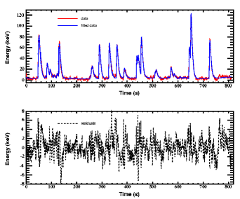
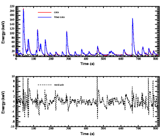
Figure 8: Sample of raw data (red) as well as best fit to the data (blue) for the A (upper panel) and B (lower panel) cells. In each case, residuals are shown below (dotted line).

5.2 Low energy conversion electron spectrum

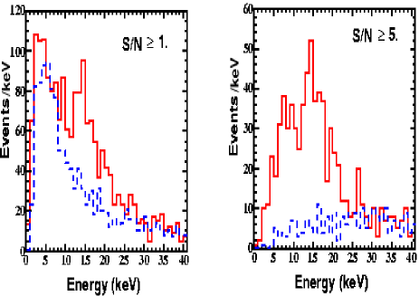
Figure 9: From left to right, we overplot the spectra for the A (blue dashed line) and B (red solid line) cells in the $[0,40]$ keV energy range for values of the $S/N$ cut of 1 and 5 respectively.

The experimental energy spectrum has been analyzed in detail in the $[0,40]$ keV energy range for both cells. The evolution of the spectrum with respect to the signal to noise cut is presented on figure 9. We plot in blue and red the energy spectrum of the A and B cells respectively. The left (resp. right) plot corresponds to a cut in the $S/N$ of 1 (resp. 5).
From the left plot, we conclude that, for a $S/N$ cut of 1, the reconstruction of the spectrum of the low energy conversion electrons is biased by spurious signals in the range from 0 to $\rm\sim 20\ keV$. This is clearly visible from the spectrum of the A cell which increases with decreasing energy. The same features were observed in the analysis of the simulated data in section 4. For a signal to noise cut of 5, the spurious signals are mostly removed from the spectrum, at a level better than 95%. This is suggested by the spectrum of the A cell which decreases toward the lowest energies as expected both from the decrease of efficiency of detection and from the negligible contribution from spurious signals discussed in section 4.5. Notice in here that the activity of the source was not accurately previously known and was estimated from this analysis. Hence, only qualitative comparison between simulation and data can be done at this stage. By comparing with figure 6, we can highlight that the lines for the conversion electrons at 7.3 and 13.6 keV are recovered. The reconstructed relative intensity between these two lines does not match what observed in the simulations. This is due to the fact that for the data spectrum the line at $\sim 13$ keV is the combination of the conversion electron line at 13.6 keV and of an extra line from the Auger electrons from the Au foil on which the source was deposited. Equally, two extra lines are present, corresponding to the physical pile-up of the conversion and Au-Auger electron lines. The contribution from the Au-Auger electrons was not taken into account in the simulation spectrum.
A more detailed analysis and physical interpretation of this spectrum as the detection of low energy conversion electrons in ${}^{3}{\mathrm{He}}$ at ultra low temperature can be found in Moulin et al. 2005b .

6 Conclusion

We present in this paper the design and implementation of a data analysis method to reconstruct highly piled-up bolometric peak-like signals from time ordered data. This method consists of three main steps: 1) wavelet based denoising to remove the high frequency noise in the data, 2) reconstruction and subtraction of the low frequency drift in the data from the local minima to avoid the bias in the amplitude of the reconstructed signal, 3) an iterative detection and fitting procedure. The detection is performed in the derivative of the residuals and for the fit we use a reference peak directly extracted from the data. For each reconstructed signal we compute its time position, amplitude and $S/N$ ratio of detection defined as the amplitude of the peak over the maximum of the residuals in the interval of detection.

The method has been applied to simulated data of the MACHe3 prototype experiment in two configurations: 1) large amplitude signals (from 10 to 120 keV) with low level of pile-up (cell A) and 2) small (few keV) and large amplitude signal with high level of pile-up. From this we have proved that the method is able to recover the lowest-amplitude simulated signals of few keVs for a rms noise of 1 keV. Considering a $S/N$ cut of 5, the efficiency of detection in the A cell (resp. B cell) configuration is above 90 % (resp. 60 %) and the contamination by spurious signals below 5 %. (resp. 1 %).

For the B cell and for a $S/N$ cut of 5 the efficiency of detection of the low amplitude simulated signals between 5-10 keV is above 50 % with negligible spurious contribution. For the same $S/N$ cut in the range from 1 to 5 keV, although we have no spurious signal, the efficiency of detection is too low because of the high level of pile-up. This does not mean that we are not able to detect low amplitude simulated signals but that we are limited by the pile-up in this analysis. For example, if we consider a $S/N$ cut of 2 the efficiency of detection is above 60 % but we have to tolerate about 20 % of spurious signal. In the case of dark matter detection, in underground laboratories, there would be significantly less pile-up and therefore the low amplitude signals from 1 to 5 keV could be detected and reconstructed.

We have also applied the method to the raw data of the MACHe3 prototype experiment, in order to demonstrate for the first time the possibility of measure low energy events (5-10 keV) in ${}^{3}{\mathrm{He}}$ at ultra-low temperature ($\rm 100\ \mu K$) Moulin et al. 2005b . Indeed, we were able to detect events corresponding to conversion electrons at 7.3 and 13 keV coming from ${}^{57}{\rm{Co}}$ source embedded in the prototype and to reconstruct their energy spectrum.

The method, although developed for the analysis of the MACHe3 data, is only based on the properties of the time ordered data. As ongoing and forthcoming Dark Matter experiments present the same features in their data, this procedure could be of general interest.