New Methods for Approximating General Relativity
in Numerical Simulations of Stellar Core Collapse

Abstract

We review various approaches to approximating general relativistic effects in hydrodynamic simulations of stellar core collapse and post-bounce evolution. Different formulations of a modified Newtonian gravitational potential are presented. Such an effective relativistic potential can be used in an otherwise standard Newtonian hydrodynamic code. An alternative approximation of general relativity is the assumption of conformal flatness for the three-metric, and its extension by adding second post-Newtonian order terms. Using a code which evolves the coupled system of metric and fluid equations, we apply the various approximation methods to numerically simulate axisymmetric models for the collapse of rotating massive stellar cores. We compare the collapse dynamics and gravitational wave signals (which are extracted using the quadrupole formula), and thereby assess the quality of the individual approximation method. It is shown that while the use of an effective relativistic potential already poses a significant improvement compared to a genuinely Newtonian approach, the two conformal-flatness-based approximation methods yield even more accurate results, which are qualitatively and quantitatively very close to those of a fully general relativistic code even for rotating models which almost collapse to a black hole.

1 Introduction

Gravity is the driving force which at the end of the life of massive stars overcomes the pressure forces and causes the collapse of the stellar core. Furthermore, the subsequent supernova explosion results from the fact that various processes tap the enormous amount of gravitational binding energy released during the formation of the proto-neutron star. Therefore, gravity plays an important role during all stages of a core collapse supernova. General relativistic effects are important in this scenario and cannot be neglected in quantitative models because of the strong compactness of the proto-neutron star. It is thus essential to include a proper treatment of general relativity (GR) or an appropriate approximation in the numerical codes that one uses to study core collapse supernovae.

Stellar core collapse is also among the most promising sources of detectable gravitational waves. As the first-stage gravitational wave interferometer detectors (like TAMA300, GEO600, LIGO, or VIRGO) are already taking data, the interest in performing core collapse simulations has been further motivated by the necessity of obtaining reliable gravitational waveform predictions for detector data analysis.

In the last two decades, a number of numerical simulations of rotating stellar core collapse were performed, paying particular attention to computing gravitational wave emission (see new_03_a and references therein). Most simulations were done using simple analytic equations of state (EOS), and were either restricted to Newtonian gravity or at most approximations of full GR. Only recently there were several successful attempts to model rotating core collapse to a proto-neutron star in full GR shibata_04_a ; shibata_05_a . Multi-dimensional simulations involving a sophisticated treatment of microphysics like a tabulated EOS and neutrino transport are up to now only performed in Newtonian gravity (see, e.g., buras_06_a ).

In order to facilitate the numerical investigation of rotating stellar core collapse taking into account effects of GR in ways which are both accurate and comparatively easy to implement without having to resort to a fully relativistic formulation, in recent years a number of approximation scenarios were suggested. In this work we summarize several such methods and apply them to numerical simulations for modeling the collapse of rotating massive stellar cores. These models, which were investigated in shibata_05_a in a full GR framework, feature comparatively extreme initial masses, rotation states, and collapse parameters, and thus reach very high densities or even collapse to black holes. Therefore, this is an ideal test scenario to assess the quality of the various approximation methods of full GR.

Throughout the article, we use geometrized units with $c=G=1$ and Einstein’s summation convention.

2 Hydrodynamic equations in flux-conservative hyperbolic form

In the following we present the hydrodynamic equations in flux-conservative formulation, which govern the evolution of matter (approximated as an perfect fluid) in a dynamic spacetime $g_{\mu\nu}$. We adopt the $3+1$ formalism to foliate spacetime into a set of non-intersecting spacelike hypersurfaces $\Sigma_{\,t}$. The line element then reads

$$ds^{\,2}=g_{ij}\,dx^{\,\mu}dx^{\nu}=-\alpha^{\,2}dt^{\,2}+\gamma_{\,ij}(dx^{\,i}+\beta^{i}dt)(dx^{\,j}+\beta^{j}dt),$$ (1)

where $\alpha$ is the lapse function describing the rate of advance of time along a timelike unit vector $n^{\,\mu}$ normal to $\Sigma_{\,t}$, $\beta^{i}$ is the spacelike shift three-vector which specifies the motion of coordinates within a surface, and $\gamma_{\,ij}$ is the spatial three-metric. In the Newtonian limit $g_{\mu\nu}$ reduces to the flat metric $\hat{g}_{\mu\nu}$ with the associated flat three-metric $\hat{\gamma}_{\,ij}$.

2.1 Newtonian hydrodynamics

As primitive (physical) hydrodynamic variables of a perfect fluid we choose the rest-mass density $\rho$, the covariant three-velocity $v_{i}$ as measured by an Eulerian observer at rest in $\Sigma_{\,t}$, and the specific internal energy $\epsilon$. We introduce the following set of conserved variables:

$$D=\rho,\qquad S_{i}=\rho v_{i},\qquad\textstyle\tau=\rho(\epsilon+\frac{1}{2}v_{i}v^{\,i}).$$

Then we obtain a first-order, flux-conservative hyperbolic system of hydrodynamic equations in Newtonian gravity,

$$\frac{\partial\sqrt{\hat{\gamma}\,}\bm{U}}{\partial t}+\frac{\partial\sqrt{\hat{\gamma}\,}\bm{F}^{\,i}}{\partial x^{\,i}}=\sqrt{\hat{\gamma}\,}\bm{S},$$ (2)

where $\hat{\gamma}$ is the determinant of $\hat{\gamma}_{\,ij}$. The state vector $\bm{U}$, flux vector $\bm{F}^{\,i}$, and source vector $\bm{S}$ are given by

$$\bm{U}=[D,S_{j},\tau],\qquad\bm{F}^{i}=\left[Dv^{\,i},S_{j}v^{\,i}+\delta^{\,i}_{j}P,(\tau+P)v^{\,i}\right]\!,\qquad\bm{S}=\left[0,-\rho\frac{\partial\Phi}{\partial x^{j}},-\rho v^{\,i}\frac{\partial\Phi}{\partial x^{\,i}}\right]\!\!.$$

Here $\Phi$ is the Newtonian gravitational potential. An EOS, which relates the fluid pressure $P$ to some thermodynamically independent quantities, e.g., $P=P(\rho,\epsilon)$, closes the system of conservation equations.

2.2 General relativistic hydrodynamics

The hydrodynamic evolution of a perfect fluid in GR with four-velocity $u^{\,\mu}$, rest-mass current $J^{\,\mu}=\rho u^{\,\mu}$, and energy-momentum tensor $T^{\mu\nu}=\rho hu^{\,\mu}u^{\nu}+Pg^{\,\mu\nu}$ is determined by a system of local conservation equations,

$$\nabla_{\!\mu}J^{\,\mu}=0,\qquad\nabla_{\!\mu}T^{\mu\nu}=0,$$ (3)

where $\nabla_{\!\mu}$ denotes the covariant derivative. The quantity $h=1+\epsilon+P/\rho$ is the specific enthalpy, and the three-velocity is given by $v^{\,i}=u^{\,i}/(\alpha u^{\,0})+\beta^{i}/\alpha$. Along the same lines as in the Newtonian framework, and following the work presented in banyuls_97_a , we define the set of conserved variables as

$$D=\rho W,\qquad S_{i}=\rho hW^{\,2}v_{i},\qquad\tau=\rho hW^{\,2}-P-D.$$

In the above expressions $W=\alpha u^{\,0}$ is the Lorentz factor, which satisfies the relation $W=1/\sqrt{1-\gamma^{\,ij}v_{i}v_{\!j}}$.

Then the local conservation laws (3) can again be written as a first-order, flux-conservative hyperbolic system of hydrodynamic equations in GR gravity,

$$\frac{\partial\sqrt{\gamma\,}\bm{U}}{\partial t}+\frac{\partial\sqrt{-g\,}\bm{F}^{\,i}}{\partial x^{\,i}}=\sqrt{-g\,}\bm{S},$$ (4)

with

$$\bm{U}=[D,S_{j},\tau],\qquad\bm{F}^{\,i}=\left[D\hat{v}^{\,i}\!,S_{j}\hat{v}^{\,i}+\delta^{\,i}_{j}P,\tau\hat{v}^{\,i}+Pv^{\,i}\right]\!,\qquad\bm{S}=\left[0,T^{\mu\nu}\!\!\left(\!\frac{\partial g_{\nu j}}{\partial x^{\,\mu}}-\Gamma^{\,\lambda}_{\!\mu\nu}g_{\lambda j}\right)\!\!,\alpha\left(T^{\mu 0}\frac{\partial\ln\alpha}{\partial x^{\,\mu}}-T^{\mu\nu}\Gamma^{\,0}_{\!\mu\nu}\!\!\right)\!\right]\!\!.$$

Here $\hat{v}^{\,i}=v^{\,i}-\beta^{i}/\alpha$, and $g$ and $\gamma$ are the determinant of $g_{ij}$ and $\gamma_{\,ij}$, respectively, with $\sqrt{-g}=\alpha\sqrt{\gamma}$. In addition, $\Gamma^{\,\lambda}_{\!\mu\nu}$ are the Christoffel symbols associated with $g_{\mu\nu}$.

3 Gravitational field equations

3.1 Effective relativistic potential for Newtonian simulations

Method N: Newtonian potential for a self-gravitating fluid.  The Newtonian potential $\Phi$, whose gradient acts as an external force in the source of the Newtonian hydrodynamic equations (2), is determined by the Poisson equation

$$\Delta\Phi=4\pi\rho.$$ (5)

To approximately include effects of GR gravity, several successful attempts of increasing complexity have been made rampp_02_a ; marek_06_a ; mueller_06_a to replace the regular Newtonian potential $\Phi$ (called method N here), by an effective relativistic gravitational potential $\Phi_{\mathrm{eff}}$ for a self-gravitating fluid, which mimics the deeper gravitational well of the GR case.

Method R: TOV potential for a self-gravitating fluid.  As a first approximation, we demand that $\Phi_{\mathrm{eff}}$ in spherical symmetry reproduces the solution of hydrostatic equilibrium according to the Tolman–Oppenheimer–Volkoff (TOV) equation. To obtain an effective relativistic potential also for a nonspherical matter distribution, we construct a generalized TOV potential rampp_02_a as a radial integral over angular averaged matter quantities $\overline{\!\rho}$, $\overline{\!\epsilon}$, $\overline{v_{r}}$, and $\overline{\!P}$:

$$\overline{\!\Phi\!}\,_{\mathrm{\,TOV}}(r)=-\int_{r}^{\,\infty}\frac{dr\,^{\prime}}{r\,^{\prime\,2}}\left(\overline{\!m}+4\pi r\,^{\prime\,3}\overline{\!P}\right)\frac{\overline{\!h}}{\overline{\Gamma}^{\,2}}.$$ (6)

Here $\overline{v_{r}}$ is the local radial velocity of the fluid. The TOV mass $\overline{\!m}$ and metric function $\overline{\Gamma}$ are given by

$$\overline{\!m}(r)=4\pi\int_{0}^{\,r}dr\,^{\prime}\,r\,^{\prime\,2}\,\overline{\!\rho}\left(1+\overline{\!\epsilon}\right),\qquad\overline{\Gamma}=\sqrt{1+\overline{v_{r}}^{\,2}-\frac{2\overline{\!m}}{r}}.$$ (7)

Then the effective relativistic potential $\Phi_{\mathrm{eff}}$ can be calculated by substituting the “spherical contribution”

$$\overline{\!\Phi\!}\,(r)=-4\pi\int_{0}^{\,\infty}\!\!\mathrm{d}r\,^{\prime}\,r\,^{\prime\,2}\,\frac{\overline{\!\rho}}{|r-r\,^{\prime}|}$$ (8)

to the multi-dimensional Newtonian gravitational potential $\Phi$ by the TOV potential $\overline{\!\Phi\!}\,_{\mathrm{\,TOV}}$:

$$\Phi_{\mathrm{eff}}=\Phi-\overline{\!\Phi\!}\,+\overline{\!\Phi\!}\,_{\mathrm{\,TOV}}.$$ (9)

When this reference case of the effective relativistic potential, method R, is used in an otherwise Newtonian simulation, the collapse of a spherical stellar core to a proto-neutron star yields after core bounce and ring-down a new quasi-equilibrium state which is the exact (numerical) solution of the TOV structure equations of GR.

The effective relativistic potential of method R has already been used in simulations of supernova core collapse in spherical symmetry with sophisticated microphysics including Boltzmann neutrino transport rampp_02_a ; liebendoerfer_05_a as well as for rotating stellar core collapse with a simple matter treatment without magnetic fields marek_06_a and with magnetic fields obergaulinger_06_a .

Method A: Modifications of the TOV potential.  In a recent comparison liebendoerfer_05_a of supernova core collapse in spherical symmetry it was found that the use of the effective relativistic potential in the form (9) overrates the relativistic effects, because in combination with Newtonian kinematics it tends to overestimate the infall velocities and to underestimate the flow inertia in the preshock region. As a consequence, the compactness of the proto-neutron star is overestimated.

In order to reduce these discrepancies, several modifications of the spherical TOV potential (6) have been tested recently marek_06_a . In all cases the construction of the multi-dimensional effective relativistic potential $\Phi_{\mathrm{eff}}$ according to Eq. (9) remains unchanged. In the most accurate of the variations introduced in marek_06_a , method A, an additional factor $\overline{\Gamma}$ is added in the integrand of the equation for the TOV mass (7). Since $\overline{\Gamma}<1$ this reduces the gravitational TOV mass used in the TOV potential (6), and thus attenuates the relativistic corrections in the effective relativistic potential $\Phi_{\mathrm{eff}}$.

As a consequence, a Newtonian simulation of core collapse using the effective relativistic potential of method A not only reproduces the solution of the TOV structure equations for a matter configuration in equilibrium to fair accuracy, but contrary to method R also closely matches the results from a relativistic simulation during the dynamic phase of the contraction of the core. This has been demonstrated in numerical studies of collapsing stellar cores in spherical symmetry with sophisticated microphysics including Boltzmann neutrino transport marek_06_a .

The results presented in that work also demonstrate that in axisymmetric collapse calculations for rotating stellar cores with a wide range of initial conditions and a simple EOS, the new effective relativistic potential of method A reproduces the characteristics of the relativistic collapse dynamics quantitatively much better than the Newtonian potential for not too rapid rotation.

3.2 Conformal-flatness-based approximations for general relativistic simulations

In the $3+1$ formalism, the Einstein equations split into a coupled set of 12 evolution equations for the three-metric $\gamma_{\,ij}$ as well as the extrinsic curvature $K_{\,ij}$, and 4 constraint equations. We use the ADM gauge, where $\gamma_{\,ij}$ can be decomposed into a conformally flat term with conformal factor $\phi$ plus a transverse traceless term:

$$\gamma_{\,ij}=\phi^{4}\hat{\gamma}_{\,ij}+h^{\mathrm{TT}}_{\,ij},\qquad\qquad\mbox{with}\qquad h^{\mathrm{TT}}_{\,ij}\hat{\gamma}^{\;ij}=0,\qquad\hat{\gamma}^{\;ik}\hat{\nabla}_{\!k\,}h^{\mathrm{TT}}_{\,ij}=0,$$ (10)

Method CFC: Conformal flatness condition for the three-metric.  In spherical symmetry $h^{\mathrm{TT}}_{\,ij}=0$, i.e. the three-metric is conformally flat. Thus a reasonable approximation of $\gamma_{\,ij}$ for scenarios which do not deviate to strongly from sphericity is to impose a vanishing $h^{\mathrm{TT}}_{\,ij}$ in Eq. (10):

$$\gamma_{\,ij}=\phi^{4}\hat{\gamma}_{\,ij}.$$ (11)

This is the conformal flatness condition (CFC) or Isenberg–Wilson–Mathews approximation isenberg_78_a ; wilson_96_a . Using CFC and assuming the maximal slicing condition, for which the trace of the extrinsic curvature vanishes, the $3+1$ metric equations reduce to a set of five coupled elliptic (Poisson-like) equations for the metric components,

$$\hat{\Delta}\phi = -2\pi\phi^{5}\left(\rho hW^{\,2}-P+\frac{K_{\,ij}K^{\,ij}}{16\pi}\right)\!,$$ (12)

$$\hat{\Delta}(\alpha\phi) = 2\pi\alpha\phi^{5}\left(\rho h(3W^{\,2}-2)+5P+\frac{7K_{\,ij}K^{\,ij}}{16\pi}\right)\!,$$ (13)

$$\hat{\Delta}\beta^{i} = 16\pi\alpha\phi^{4}S^{\,i}+2\phi^{10}K^{\,ij}\hat{\nabla}_{\!\!j}\!\left(\!\frac{\alpha}{\phi^{6}}\!\right)\!-\frac{1}{3}\hat{\nabla}^{i\,}\hat{\nabla}_{\!k\,}\beta^{k}\!,$$ (14)

where $\hat{\nabla}$ and $\hat{\Delta}=\hat{\gamma}^{\;ij}\hat{\nabla}_{i\,}\hat{\nabla}_{\!\!j}$ are the flat space Nabla and Laplace operators. Additionally, the expression for the extrinsic curvature becomes time-independent and reads $K_{\,ij}=\frac{1}{2\alpha}(\nabla_{\!i\,}\beta_{j}+\nabla_{\!\!j\,}\beta_{i}-\frac{2}{3}\gamma_{\,ij}\nabla_{\!k\,}\beta^{k})$. As the CFC metric equations (12 – 14) do not contain explicit time derivatives, the metric is calculated by a fully constrained approach.

The accuracy of the CFC approximation has been tested in various works, e.g., for stellar core collapse and equilibrium models of neutron stars shibata_04_a ; cook_96_a ; dimmelmeier_02_a ; dimmelmeier_05_a ; saijo_05_a ; dimmelmeier_06_a , as well as for binary neutron star merger oechslin_02_a ; faber_04_a . The spacetime of rapidly (uniformly or differentially) rotating neutron star models is very well approximated by the CFC metric (11). Its accuracy degrades only in extreme cases, such as rapidly rotating massive neutron stars or black holes.

Method CFC+: Inclusion of the second post-Newtonian deviation from isotropy.  To improve the accuracy of CFC, we have developed the CFC+ approximation. It consists in adding to the CFC metric (11) the second post-Newtonian (2PN) deviation from isotropy,

$$\gamma_{\,ij}=\phi^{4}\hat{\gamma}_{\,ij}+h^{\mathrm{\,2PN}}_{\,ij}$$ (15)

which includes a traceless and transverse term $h^{\mathrm{\,2PN}}_{\,ij}$. In the decomposition (10) $h^{\mathrm{\,2PN}}_{\,ij}$ is identical to $h^{\mathrm{TT}}_{\,ij}$ up to 2PN order. As described in detail in cerda_05_a this correction is the solution of the tensor Poisson equation schaefer_90_a

$$\hat{\Delta}h^{\mathrm{\,2PN}}_{\,ij}=\hat{\gamma}_{\,ij}^{\mathrm{\,TT}kl}\left(\!-4\hat{\nabla}_{\!k\,}U\,\hat{\nabla}_{\!l\,}U-16\pi\left(S^{*}_{k}S^{*}_{l}\right)/D^{*}\!\right)\!,$$ (16)

where $U$ is a Newtonian-like potential which is the solution of the Poisson equation $\hat{\Delta}U=-4\pi D^{*}$, $D^{*}=\sqrt{\gamma/\hat{\gamma}\,}D$, and $S^{*}_{i}=\sqrt{\gamma/\hat{\gamma}\,}S_{i}$. The integro-differential operator $\hat{\gamma}_{\,ij}^{\mathrm{TT}kl}$ is the traceless and transverse projector defined in the Appendix of cerda_05_a . Of the CFC metric equations (12 – 14), only the equation (13) for the lapse function $\alpha$ is affected by the corrections $h^{\mathrm{\,2PN}}_{\,ij}$:

$$\hat{\Delta}(\alpha\phi)=\left[\hat{\Delta}\left(\alpha\phi\right)\right]_{\!h_{\,ij}^{\mathrm{\,2PN}}=0}\!-\hat{\gamma}^{\,ik}\hat{\gamma}^{\,jl}\,h^{\mathrm{\,2PN}}_{\,ij}\,\hat{\nabla}_{\!k\,}\hat{\nabla}_{\!l\,}U.$$ (17)

However, the CFC+ corrections couple implicitly to the other metric equations as their source terms depend on $\alpha$.

Calculating $h^{\mathrm{\,2PN}}_{\,ij}$ by inversion of the tensor Poisson equation (16) is simplified considerably by introducing potentials that are solutions of scalar/vector/tensor Poisson equations cerda_05_a .

Applying method CFC+ to axisymmetric simulations of pulsations in rotating neutron stars and rotational stellar core collapse to a proto-neutron star, it was recently found that relevant quantities show only minute differences with respect to method CFC cerda_05_a . By contrast, in scenarios where the CFC approximation is expected to become increasingly inaccurate, CFC+ is expected to yield results which are closer to full GR.

4 Simulations of the collapse of rotating massive stellar cores

4.1 Setup of models and numerical methods

We follow the work in shibata_05_a to set up rapidly rotating initial models of massive stellar cores with baryonic rest masses $M_{\mathrm{\,r}}\gtrsim 1.5\,M_{\odot}$, supported by electron degeneracy pressure and a possible radiation pressure contribution. Using Hachisu’s self-consistent field method komatsu_89_a , we construct the initial model as a rotating perfect fluid in equilibrium obeying a polytropic EOS, $P=K_{\,0}\rho^{\gamma_{\,0}}$ and $\epsilon=P/[\rho(\gamma_{\,0}-1)]$, where $\gamma_{\,0}=4/3$ is the adiabatic index and the polytropic constant assumes values $K_{\,0}=\{5.0,~{}7.0,~{}8.0\}\times 10^{14}$ (in cgs units) with increasing contribution from radiation pressure. The initial core’s central density is $\rho_{\mathrm{\,c\;0}}=10^{10}\mathrm{\ g\ cm}^{-3}$. The rotation law is set by $j=A^{2}(\Omega_{\mathrm{\,c}}-\Omega)$, where $j$ is the specific angular momentum, $\Omega_{\mathrm{\,c}}$ is the value of the angular velocity $\Omega$ at the center, and the constant $A$ determines the degree of differential rotation. We parameterize the rotational state by two quantities, the rotation rate $\beta_{\,0}$ which is the ratio of rotational kinetic energy to gravitational binding energy, and the parameter $\hat{A}=A/r_{\mathrm{\,e}}=\{\infty,~{}0.25,~{}0.1\}$, where $r_{\mathrm{\,e}}$ is the stellar equatorial radius, which decreases as the differentiality of the rotation profile increases (with $\hat{A}=\infty$ corresponding to uniform rotation). To initiate the collapse we reduce the pressure, $P=K_{\,0}\rho^{\gamma_{\,0}}(\gamma_{\,1}-1)/(\gamma_{\,0}-1)$, with lowering the adiabatic index to $\gamma_{\,1}=1.31<\gamma_{\,0}$ and setting the polytropic constant to $K_{\,1}=5.0\times 10^{14}$. Note that this procedure is different from the collapse initiation for the models presented in shibata_04_a ; dimmelmeier_02_a ; dimmelmeier_05_a ; cerda_05_a ; dimmelmeier_02_b , where both the pressure and the internal energy are reduced.

As in shibata_04_a ; shibata_05_a ; dimmelmeier_02_a ; dimmelmeier_05_a ; dimmelmeier_02_b , during the collapse phase we use a simple hybrid ideal gas EOS janka_93_a that consists of a polytropic contribution $P_{\mathrm{\,p}}$ describing the degenerate electron pressure and at supranuclear densities the pressure due to repulsive nuclear forces, and a thermal contribution $P_{\mathrm{\,th}}$ which accounts for the heating of the matter by shocks, $P=P_{\mathrm{\,p}}+P_{\mathrm{\,th}}$, where $P_{\mathrm{\,p}}=K_{\,1,2}\,\rho^{\gamma_{\,1,2}}$ and $P_{\mathrm{\,th}}=\rho\epsilon_{\mathrm{\,th}}(\gamma_{\mathrm{\,th}}-1)$. To approximate the stiffening of the EOS at densities larger than nuclear matter density $\rho_{\mathrm{\,nuc}}=2.0\times 10^{14}\mathrm{\ g\ cm}^{-3}$, the adiabatic index increases to $\gamma_{\,2}=2.5>\gamma_{\,1}$. For the adiabatic index of the thermal contribution we choose $\gamma_{\mathrm{\,th}}=1.3$. The thermal internal energy is calculated as $\epsilon_{\mathrm{\,th}}=\epsilon-\epsilon_{\mathrm{\,p}}$, while the polytropic specific internal energy $\epsilon_{\mathrm{\,p}}$ is determined from $P_{\mathrm{\,p}}$ by the ideal gas relation in combination with continuity conditions, which also determine the value for the polytropic constant $K_{\,2}$ at $\rho>\rho_{\mathrm{\,nuc}}$ (for more details, see dimmelmeier_02_a ; janka_93_a ). Of the 27 axisymmetric collapse models of rotating massive stellar cores investigated in shibata_05_a , here we select 8 representative models. Table 1 summarizes their parameters and establishes the nomenclature of model names.

Model	M5a1	M5c2	M7a4	M7b1	M7c3	M8a1	M8c2	M8c4
$K_{\,0}~{}[10^{14}]$	5.00	5.00	7.00	7.00	7.00	8.00	8.00	8.00
$\hat{A}$	$\infty$	0.10	$\infty$	0.25	0.10	$\infty$	0.25	0.10
$\beta_{\,0}~{}[\%]$	0.89	1.24	3.67	2.18	1.27	0.88	2.19	1.27

Table 1: Summary of the model parameters for rotating massive stellar cores.

Our evolution code, which was introduced in dimmelmeier_02_a ; cerda_05_a , utilizes Eulerian spherical polar coordinates $\{r,\theta\}$ restricted to axisymmetry. We also assume symmetry with respect to the equatorial plane. The finite difference grid consists of $n_{r}=250$ logarithmically spaced radial and $n_{\theta}=45$ equidistantly spaced angular grid points with a central resolution $\Delta r_{\mathrm{\,c}}\simeq 250\mathrm{\ m}$. A small part of the grid covers an artificial low-density atmosphere extending beyond the stellar surface.

The hydrodynamic solver performs the time integration of the system of conservation equations, given either by Eq. (2) for methods N, R, and A, or by Eq. (4) for methods CFC and CFC+. This is done by means of a high-resolution shock-capturing (HRSC) scheme with third-order accurate PPM reconstruction (for a review of such methods in numerical GR, see font_03_a ). The numerical fluxes are computed by Marquina’s approximate flux formula donat_98_a . The time update of the state vector $\bm{U}$ is done using the method of lines in combination with a Runge–Kutta scheme with second order accuracy in time. Once $\bm{U}$ is updated in time, the primitive variables are recovered either directly (for methods N, R, and A) or through an iterative Newton–Raphson method (for methods CFC and CFC+).

When using methods N, R, or A we solve the multi-dimensional linear Poisson equation (5) for the Newtonian potential $\Phi$ by transforming it into an integral equation using a Green’s function. The volume integral is numerically evaluated by expanding the source term into a series of radial functions and associated Legendre polynomials, which we cut at order $l=10$. It is straightforward to solve the integral equations (6 – 8) of the relativistic corrections needed to finally obtain the effective relativistic potential $\Phi_{\mathrm{eff}}$.

The metric solver for obtaining the CFC and CFC+ spacetime metric used in the GR simulations exploits the fact that Eqs. (12 – 14), supplemented by Eqs. (16, 17) in the case of method CFC+, are written in the form of a system of nonlinear coupled equations for a vector of unknowns $\bm{u}$ with a Laplace operator on the left hand side, $\hat{\Delta}\,\bm{u}=\bm{S}(\bm{u})$. A common method to solve such equations is to keep $\bm{S}(\bm{u})$ fixed, start with an initial guess $\bm{u}^{\,0}$, and then solve each of the resulting decoupled linear Poisson equations $\hat{\Delta}\,\bm{u}^{\,s+1}=\bm{S}(\bm{u}^{\,s})$ in an iteration cycle with steps $s$ until convergence. To obtain the solution of the now uncoupled, linear Poisson equations, we again employ the expansion described above. More details are presented in the description of Solver 2 in dimmelmeier_05_a .

The calculation of the CFC or CFC+ metric is computationally very expensive. Hence, for these methods the metric is updated only once every 100/10/50 hydrodynamic time steps before/during/after core bounce, and extrapolated in between, as described in dimmelmeier_02_a . We also note that we have performed grid resolution tests to ascertain that the grid resolution specified above is appropriate. When using the CFC/CFC+ metric equations, the degrees of freedom representing gravitational waves are removed from the spacetime. Therefore, in all simulations gravitational waveforms are obtained in a post-processing step with the help of the quadrupole formula.

4.2 Results and discussion

Comparing typical quantities that describe the collapse dynamics (like the maximum density $\rho_{\mathrm{\,max\;b}}$, maximum rotation rate $\beta_{\mathrm{\,max\;b}}$, or minimal value of the lapse $\alpha_{\mathrm{\,min\;b}}$ during core bounce) from our approximate GR simulations with those obtained in full GR shibata_05_a , we find excellent agreement for both method CFC and CFC+. In the case of models which do not collapse to a black hole, our results for $\rho_{\mathrm{\,max\;b}}$ (which we present in Table 2) deviate from the full GR ones by typically less than about 2% for models with moderate core mass and moderate or rapid rotation. The deviation for $\rho_{\mathrm{\,max\;b}}$ increases to at most 20% for the most extreme model M8c4, which has a baryonic rest mass of $M_{\mathrm{\,r}}=3.05$ and a slow rotation rate. Consequently, this model reaches $\alpha_{\mathrm{\,min}}=0.29$ and thus almost collapses to a black hole.

Model	Method N		Method R		Method A		Method CFC		Method CFC+		GR
M5a1	3.8	(0.58)	6.1	(0.92)	5.6	(0.85)	6.6	(1.00)	6.6	(1.00)	6.6
M5c2	1.1	(0.22)	3.3	(0.66)	2.9	(0.58)	4.9	(0.98)	4.9	(0.98)	5.0
M7a4	5.6	—	—	—	14	—	14	—	14	—	—
M7b1	0.10	(0.13)	0.40	(0.51)	0.31	(0.39)	0.83	(1.05)	0.85	(1.08)	0.79
M7c3	1.2	(0.13)	5.3	(0.58)	4.2	(0.46)	9.2	(1.00)	9.2	(1.00)	9.2
M8a1	4.5	—	—	—	17	—	—	—	—	—	—
M8c2	0.19	(0.04)	1.5	(0.28)	9.0	(0.17)	5.3	(0.98)	5.2	(0.96)	5.4
M8c4	1.2	(0.08)	7.1	(0.47)	5.1	(0.34)	17	(1.13)	12	(0.80)	15

Table 2: Maximum density $\rho_{\mathrm{\,max\;b}}$ in units of $10^{14}\mathrm{\ g\ cm}^{-3}$ during core bounce for the investigated rotating core collapse models from simulations using methods N, R, A, CFC, and CFC+. The relative deviations $\rho_{\mathrm{\,max\;b}}/\rho_{\mathrm{\,max\;b}}^{\mathrm{GR}}$ from the value obtained in a full GR simulation (given in the last column) are shown in parentheses. The dash denotes models for which the approximate or full GR simulation produces a black hole.

When the less accurate approximation methods A and R are used, the values for $\rho_{\mathrm{\,max\;b}}$ as expected deviate more strongly from full GR and approach the ones obtained using a genuinely Newtonian simulation. Concerning the quality of our approximations, we find equivalent results for the values of $\rho_{\mathrm{\,max\;b}}$, $\beta_{\mathrm{\,max\;b}}$, and $\alpha_{\,min\;b}$ (with the latter obviously only defined for methods CFC and CFC+). Note also that though method A compared to method R yields results closer to full GR in spherical symmetry, the influence of rotation reverses this behavior, as already discussed in marek_06_a .

A very important property of any approximation method for GR simulations is that it should correctly reproduce the collapse type of a specific model for a range in parameter space as broad as possible. For the investigated models, following shibata_05_a we denote by BH, NS, O-A, and O-B the collapse to a black hole, a neutron star, an oscillating star with $\rho_{\mathrm{\,max\;b}}\geq\rho_{\mathrm{\,nuc}}$, and an oscillating star with $\rho_{\mathrm{\,max\;b}}<\rho_{\mathrm{\,nuc}}$ as end state, respectively. As shown in Table 3, methods CFC and CFC+ correctly capture the collapse type for all investigated cases. The identification of the end state of model M7a4 (as well as of model M7a3) as a black hole in shibata_05_a is most probably due to insufficient resolution of the inner parts of the numerical grid, which results in fall-back to the already formed proto-neutron star leading to its recollapse to a black hole. We find that behavior in a resolution study of these two models. This is also supported by independent simulations in full GR without symmetry assumptions shibata_05_b . We thus classify model M7a4 as NS.

Model	Method N	Method R	Method A	Method CFC	Method CFC+	GR
M5a1	NS	NS	NS	NS	NS	NS
M5c2	O-B	O-A	O-A	O-A $\rightarrow$ NS	O-A $\rightarrow$ NS	O-A $\rightarrow$ NS
M7a4	NS	BH	NS	NS	NS	NS / BH
M7b1	O-B	O-B	O-B	O-B	O-B	O-B
M7c3	O-B	NS	O-A $\rightarrow$ NS	NS	NS	NS
M8a1	NS	BH	NS	BH	BH	BH
M8c2	O-B	O-B	O-B	O-A	O-A	O-A
M8c4	O-B	NS	NS	NS	NS	NS

Table 3: Collapse type of the investigated rotating core collapse models from simulations using methods N, R, A, CFC, and CFC+. The simulations which yield the correct collapse type obtained in a full GR simulation (given in the last column) are marked by a box. See the main text for the definition of the collapse types. For model M7a4 the full GR simulation in shibata_05_a predicts BH instead of NS as final state, which is apparently due to lack of resolution.

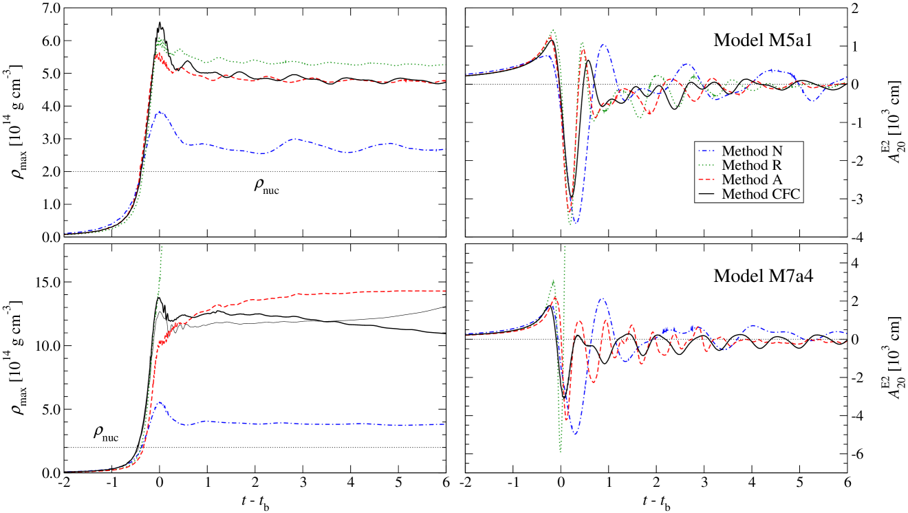
Figure 1: Time evolution of the maximum density $\rho_{\mathrm{max}}$ (left panels) and the gravitational wave signal amplitude $A^{\mathrm{E2}}_{20}$ (right panels) for the rotational core collapse models M5a1 (top panels) and M7a4 (lower panels) from simulations using method N (blue dash-dotted lines), method R (green dotted lines), method A (red dashed lines), and method CFC (black solid lines). The thin black solid line in the left bottom panel shows $\rho_{\mathrm{max}}$ for model M7a4 using method CFC in low resolution.

Fig. 1 displays the time evolution of the maximum density $\rho_{\mathrm{\,max}}$ and the gravitational wave signal amplitude $A^{\mathrm{E2}}_{20}$ (i.e. the gravitational radiation waveform; for a definition of $A^{\mathrm{E2}}_{20}$, see, e.g., dimmelmeier_02_b ) for models M5a1 and M7a4, which are all of collapse type NS in a full GR simulation. As the results of method CFC and CFC+ are almost identical, we do not show the latter in Fig. 1. We emphasize that even for these rather extreme stellar core collapse models, the 2PN deviation from isotropy in method CFC+ remains very small, $h^{\mathrm{\,2PN}}_{\,ij}\sim 0.001\mbox{\,--\,}0.01\ll 1$. Only for models like M8c4 which reach extremely high densities and low values of the lapse function, the components of $h^{\mathrm{\,2PN}}_{\,ij}$ increase to 0.02. This further supports the observation that method CFC already is an excellent approximation of full GR. For all models the purely Newtonian simulation, method N, yields maximum densities far below the values in CFC both during and after core bounce. These results for rotating massive stellar cores are in accordance with the findings for rotating regular stellar cores in dimmelmeier_02_b ; dimmelmeier_01_a . There the typically higher waveform amplitudes at core bounce in method N compared to method CFC for many models of type NS, observed here as well in Fig. 1, are also found and explained.

In model M5a1 (top panel) the post-bounce value of $\rho_{\mathrm{max}}$ for approximation method A matches best the result with method CFC, which (with method CFC+) is closest to full GR, while method R gives too large values. A similar behavior was found and discussed for the rotating core collapse model A1B3G1 in marek_06_a . The inadequacy of method R for reproducing the collapse type of certain models is evident for model M7a4 (bottom panel), where the collapse proceeds unhalted and thus the prompt formation of a black hole is predicted, while the other approximation methods capture the collapse type right. Beyond employing a good approximation of GR, it is also crucial to use a numerical grid with sufficiently accuracy. On a grid with a low central and global resolution of $n_{r}=100$, $n_{\theta}=20$, and $\Delta r_{\mathrm{\,c}}\simeq 500\mathrm{\ m}$, the core of model M7a4 (and many other models as well) simulated in method CFC suffers from matter fall-back after core bounce, recollapses, and predicts the delayed formation of a black hole as in shibata_05_b (see left bottom panel of Fig. 1).

5 Summary and outlook

We have presented several recently introduced methods for approximating GR effects in hydrodynamic simulations of stellar core collapse. When applied to axisymmetric test models for the collapse of rotating massive stellar cores which reach high densities and rotation rates, these approximations as expected offer much better results than a genuinely Newtonian treatment of gravity. While the accuracy of methods using an effective relativistic potential in an otherwise Newtonian code degrades at rapid rotation (which can be remedied by a new formulation mueller_06_a ) and these methods reach their limit for high densities and/or strong rotation, approximations based on conformal flatness prove to yield excellent matching with full GR for all investigated models.

References

- (1) C. L. Fryer, and K. C. B. New, Living Rev. Relativ., 6, 2 (2003); http://www.livingreviews.org/lrr-2003-2.
- (2) M. Shibata, and Y. I. Sekiguchi, Phys. Rev. D, 69, 084024 (2004).
- (3) M. Shibata, and Y. I. Sekiguchi, Phys. Rev. D, 71, 024014 (2005).
- (4) R. Buras et al., Astron. Astrophys., 447, 1049 (2006).
- (5) F. Banyuls et al., Astrophys. J., 476, 221 (1997).
- (6) M. Rampp, and H.-T. Janka, Astron. Astrophys., 396, 361 (2002).
- (7) A. Marek et al., Astron. Astrophys., 445, 273 (2006).
- (8) B. J. Müller, H. Dimmelmeier, and E. Müller, in preparation (2006).
- (9) M. Liebendörfer et al., Astrophys. J., 620, 840 (2005).
- (10) M. Obergaulinger et al., Astron. Astrophys., submitted (2006); astro-ph/0602187.
- (11) J. A. Isenberg, “Waveless approximation theories of gravity”, University of Maryland Preprint, unpublished (1978).
- (12) J. R. Wilson, G. J. Mathews, and P. Marronetti, Phys. Rev. D, 54, 1317 (1996).
- (13) G. B. Cook, S. L. Shapiro, and S. A. Teukolsky, Phys. Rev. D, 53, 5533 (1996).
- (14) H. Dimmelmeier, J. A. Font, and E. Müller, Astron. Astrophys., 388, 917 (2002).
- (15) H. Dimmelmeier et al., Phys. Rev. D, 71, 064023 (2005).
- (16) M. Saijo, Phys. Rev. D, 71, 104038 (2005).
- (17) H. Dimmelmeier, N. Stergioulas, and J. A. Font, Mon. Not. R. Astron. Soc., accepted (2006); astro-ph/0511394.
- (18) R. Oechslin, S. Rosswog, and F.-K. Thielemann, Phys. Rev. D, 65, 103005 (2002).
- (19) J. A. Faber, P. Grandclément, and F. A. Rasio, Phys. Rev. D, 69, 124036 (2004).
- (20) P. Cerdá-Durán et al., Astron. Astrophys., 439, 1033 (2005).
- (21) G. Schäfer, Astron. Nachr., 311, 213 (1990).
- (22) H. Komatsu, Y. Eriguchi, and I. Hachisu, Mon. Not. R. Astron. Soc., 237, 335 (1989).
- (23) H. Dimmelmeier, J. A. Font, and E. Müller, Astron. Astrophys., 393, 523 (2002).
- (24) H.-T. Janka, T. Zwerger, and R. Mönchmeyer, Astron. Astrophys., 268, 360 (1993).
- (25) J. A. Font, Living Rev. Relativ., 6, 4 (2003); http://www.livingreviews.org/lrr-2003-4.
- (26) R. Donat et al., J. Comput. Phys., 146, 58 (1998).
- (27) M. Shibata, and C. D. Ott, private communication (2005).
- (28) H. Dimmelmeier, J. A. Font, and E. Müller, Astrophys. J. Lett., 560, L163 (2001).