A Century of Cosmology

Abstract

In the century since Einstein’s anno mirabilis of 1905, our concept of the Universe has expanded from Kapteyn’s flattened disk of stars only 10 kpc across to an observed horizon about 30 Gpc across that is only a tiny fraction of an immensely large inflated bubble. The expansion of our knowledge about the Universe, both in the types of data and the sheer quantity of data, has been just as dramatic. This talk will summarize this century of progress and our current understanding of the cosmos.

1 Introduction

When the COBE DMR results were announced in 1992, Hawking was quoted in The Times stating that ”It was the discovery of the century, if not of all time.” But the progress in cosmology in the last century has been tremendous, going far beyond the anisotropy of the cosmic microwave background. A century ago the “Structure of the Universe” meant the patterns of stellar number counts and proper motions that delineated the discus-shaped distribution of observed stars [1]. The true scale of the Milky Way and the nature of the extragalactic nebulae were yet to be determined. As late as 1963 people could say that there were only 2.5 facts in cosmology [2]: 1) the sky is dark at night, 2) the redshifts of galaxies show a pattern consistent with a general expansion of the Universe, and 2.5) the Universe has evolved over time. In 1963 the controversy between the Steady State [3,4] and the Big Bang [5,6] models of cosmology was still quite active, so the last item in the list was only a half-fact.

2 Einstein and $\lambda$

Once Einstein developed general relativity, giving a theory for classical gravity, he worked out a cosmological model [7] using what was then known about the Universe. Einstein assumed that the Universe had to be homogeneous, since even if the matter were confined to a finite region initially, the action of gravitational scattering would lead to stars being ejected from the initial distribution. Since the solution of Poisson’s equation for a uniform density extending to infinity is not well defined, Einstein considered modifying Newtonian gravity by adding a $\lambda$ term, giving $\nabla^{2}\phi-\lambda\phi=4\pi G\rho$, which has the constant solution $\phi=-4\pi G\rho/\lambda$ for constant density. This modified Newtonian gravity has a short range compared to the infinite range inverse square law behavior of normal gravity. But in General Relativity the $\lambda$ term had to be multiplied not by $\phi$, which is not covariant, but rather by the metric $g_{\mu\nu}$ which contains $\phi$ as $g_{00}\approx 1+2\phi/c^{2}$ in the Newtonian approximation. Einstein found that for a uniform distribution of matter the geometry of space was that of the 3-sphere $S^{3}$ (the surface of a 4 dimensional ball), and that the addition of the $\lambda$ term could compensate for the tendency for the Universe to collapse.

This static, spherical, homogeneous and isotropic Einstein Universe was not compatible with a solution to Olbers’ Paradox. The stars in the Universe were emitting light, and this light would circulate around the spherical Universe and never be lost. As the stars continued to emit light, the Universe would become brighter and brighter. In addition to not solving Olbers’ Paradox, Einstein’s static Universe was only a unstable equilibrium point between a collapsing model and an infinitely expanding model. After the redshift of distant galaxies was discovered [8], Einstein referred to the introduction of $\lambda$ as his greatest blunder.

Other cosmological models were developed as well. The de Sitter Universe used only $\lambda$ and had no matter [9]. It has a redshift growing with distance, consistent with the Hubble Law, and this metric is now recognized as a homogeneous and isotropic Euclidean space (“flat” space means a 3 dimensional Euclidean geometry) that is expanding exponentially with time. The metric of the Steady State model is exactly the same as the de Sitter metric, but since the Steady State model has both matter and the continuous creation of new matter, the $\lambda$ term was replaced with a $C$-field that made the matter plus $C$-field in the Steady State be equivalent to the pure vacuum energy of the de Sitter space..

Friedmann introduced models with matter that expanded from an initial singularity [10]. These models show a redshift proportional to distance which is consistent with the Hubble Law.

3 Big Bang vs. Steady State

After World War II Gamow tried to use the new knowledge about nuclear physics in a cosmological context. He and his students considered first a Universe full of neutrons that expanded and decayed. But they changed to a Universe initially filled with a hot dense medium about equally split between neutrons and protons. As the Universe expanded and cooled, heavier elements would be formed by the successive addition of neutrons. In this model, nuclei with high neutron capture cross-sections would be rapidly converted into heavier nuclei, and would thus be rare in the current Universe. Indeed, a roughly inverse relation between abundance and neutron capture cross section is observed. The time vs temperature during the cooling is related to the matter to radiation ratio in the Universe, and then by estimating the current density of matter, it was possible to estimate the current temperature of Universe [6] as 1 K or 5 K.

In this model, the current Universe is more or less curvature dominated so the ratio $\Omega=\rho/\rho_{crit}$ is $<<1$ and therefore the age of the Universe is $t_{\circ}\approx 1/H_{\circ}=978\;\mbox{Gyr}/H_{\circ}\;\mbox{in km/sec/Mpc}$. Since the value of the Hubble constant given by Hubble was $\approx 500\;\mbox{km/sec/Mpc}$ the age of the Universe was about 2 Gyr, which was too short according to the radioactive dating of the Earth. In the Steady State model the scale factor of the Universe is an exponential function of time, $a(t)=\exp(H(t-t_{\circ}))$, and thus the Hubble constant is actually a constant and the age of the Universe is infinite. But the average age of the matter in the Universe is in fact quite short: $\langle\tau\rangle=1/3H\approx 700\;\mbox{Myr}$ for Hubble’s value of the Hubble constant. Taking 6 Gyr as a minimum age for the Milky Way based on the radioactive dating of the Earth and adding time needed to form the galaxy and stars, the probability that a random piece of the Universe would be that old or older was only $e^{-9}\approx 10^{-4}$ in the Steady State model but this was still better than the zero probability in the Big Bang model.

4 Discovery and Non-discovery of the CMB

The first evidence [11] for the CMB was a rather inconspicuous interstellar absorption line in the spectrum of the hot, rapidly rotating star $\zeta$ Oph. This line was identified with the R(1) line of the cyanogen radical, CN. It was rather unusual, since it arises from a rotationally excited state of CN. Given the low density of the interstellar medium, ions and molecules in the ISM spend almost all of the time in the ground state. The excitation temperature [12] of the rotational transition based on this first CN data was 2.3 K, but its cosmological significance was widely ignored. Nobel Prize winner Herzberg stated: “From the intensity ratio of the lines with K=0 and K=1 a rotational temperature of $2.3^{\circ}$ K follows, which has of course only a very restricted meaning.” But it is not true that the cosmological significance was completely ignored. In fact Hoyle, in a review [13] of a book by Gamow & Critchfield, wrote that “the authors use a cosmological model in direct conflict with more widely accepted results. The age of the Universe is this model is appreciably less than the agreed age of the Galaxy. Moreover it would lead to a temperature of the radiation at present maintained throughout the whole of space much greater than McKellar’s determination for some regions within the Galaxy.” In making this statement Hoyle ignored the careful and explicit calculations of $T_{\circ}$ contained in a refereed article [6], which were perfectly compatible with the CN temperature measured by McKellar. I find it remarkable that none of the parties involved thought to follow up this possibility of a decisive test of the Big Bang vs. Steady State.

As a result, the actual discovery of the CMB was left to Penzias & Wilson, who were quite dedicated to finding the source of the excess noise they saw in their low-noise microwave receiver. Within 7 months of the announcement of Penzias & Wilson’s result, the brightness temperature of the CMB at the 2.6 mm wavelength of the CN rotational transition had been shown to be the same as that measured at 7.4 cm by Penzias & Wilson. And thus Gamow, Alpher, Herman and Hoyle all missed the Nobel Proze.

Bob Dicke also narrowly missed the Nobel Prize. He invented the Dicke radiometer used in all direct measurements of the CMB spectrum, and during World War II came within a factor of ten of discovering the CMB, even while working from a sea level location in Florida [14]. While building a radiometer with a cold load to specifically search for the CMB, Dicke, Roll, Peebles & Wilkinson heard from Penzias & Wilson about their work.

5 Nucleosynthesis

Since Gamow’s motivation for the Big Bang model was the origin of the chemical elements, it is instructive to see how the Big Bang and Steady State models fare on isotopic abundances. One cannot make isotopes heavier than ${}^{4}He$ by the sequential addition of neutrons in the Big Bang because there is no nucleus with atomic weight $A=5$ that is even slightly stable. Thus the Big Bang, which set out to explain the abundances of the elements from hydrogen to uranium ended up only able to produce the elements from hydrogen to helium, with a sprinkling of lithium.

The Steady State model, on the other hand, proposed that matter was continuously created in the form of hydrogen, and that all heavier elements were created in stars. The triple-$\alpha$ reaction, ${}^{4}He+{}^{4}He+{}^{4}He\rightarrow{}^{12}C$, can run in stars because conditions of high density and high temperature persist for a long time. Thus all the elements can be produced in stars, starting by fusing hydrogen into helium. Stars produce about 1 gram of elements heavier than helium (“metals” to an astronomer) for each 3 grams of helium. But the average helium to metals ratio is about 12 to 1, and in low metallicity stars the ratio is even higher. Thus the Steady State model fails to produce enough helium, leading to the “helium problem”. A proposed solution [15] to this problem was to have the ongoing creation of matter in the Steady State model occur sporadically in a number of “little bangs” that produce a mixture of hydrogen and helium.

The current model uses a combination of Big Bang nucleosynthesis, which produces most of the helium, and stellar nucleosynthesis, which produces the metals and some helium. Nuclear reactions during the Big Bang, starting from a mixture of protons and neutrons in thermal equilibrium at $t<1$ sec after the Big Bang and $T>10^{10}$ K, produce the deuterium ($D$), ${}^{3}He$, ${}^{4}He$ and ${}^{7}Li$ seen in material that has not been processed through stars. Stars can destroy $D$ and ${}^{7}Li$, and generate more ${}^{4}He$. The predicted abundances depend on the number of neutrino species and the baryon to photon ratio. The number of neutrino species primarily controls the ${}^{4}He$ abundance, and appears to be 3, consistent with determinations based on the decay width of the Z boson. The baryon to photon ratio controls the D:H ratio and the ${}^{7}Li$ abundance. The baryon to photon ratio consistent with the D:H ratio seen in high redshift quasar absorption line systems appears to predict a higher ${}^{7}Li$ abundance than that observed in a certain class of stars that has been thought not to have destroyed lithium in their surface layers. But since stars certainly do destroy lithium in their interiors this discrepancy is not too serious.

6 CMB Anisotropy

The CMB was found to be remarkably isotropic. This provided strong evidence that the simple Friedmann-Robertson-Walker metrics, adopted as a useful approximation, were actually quite good representations of the real Universe. While galaxy counts in different directions as a function of brightness had already demonstrated that the Universe was homogeneous and isotropic on large scales, it was still possible in 1967 to propose 10% inhomogeneities leading to 1% anisotropies in the CMB [16]. The first detection of the CMB anisotropy was at the 0.1% level [17,18], and it was soon in textbooks [19] as due to the motion of the Solar System relative to the Universe. The alleged “discovery” of the dipole anisotropy by the U2 experiment [20] was published 6 years after the textbook. Anisotropy other than this dipole term was not detected until 1992, by the COBE DMR [21,22] at the 0.001% level.

The low level of the anisotropy seen by COBE was strong evidence for the existence of dark matter. Dark matter can start to collapse as soon as the matter density exceeds the radiation density, while baryonic matter is frozen to the photons until recombination. Thus there is more growth for structures in dark matter dominated models, and thus the currently observed large scale structure can be generated starting from smaller seeds and hence smaller CMB anisotropies [23]. But the ratio of fluctuations at supercluster scales to the fluctuations at cluster scales required a modest reduction in the small scale power that could be supplied by either an open Universe model (OCDM), a model with a mixture of hot and cold running dark matter (mixed dark matter, or MDM), or by a model dominated by a cosmological constant ($\Lambda$CDM) [22].

Detailed calculations of cold dark models (CDM) showed acoustic oscillations in the amplitude of the anisotropy as function of angular scale [24]. These oscillations were caused by an interference between the fluctuations in the dark matter, which has zero pressure and thus zero sound speed, and the baryon-photon fluid which has a sound speed near 170,000 km/sec. The angular scale of the main peak of the angular power spectrum depends on two parameters: whether the Universe is open, flat or closed ($\Omega_{tot}$), and the amount of vacuum energy density ($\Omega_{\Lambda}$).

The first observational evidence for the main acoustic peak came from a collection of data from different experiments [25]. By 2003, the WMAP experiment [26] had measured the position of the first peak to an accuracy of better than 0.5% [27]. The result requires the Universe to lie along a line segment in the $\Omega_{tot}$ vs $\Omega_{\Lambda}$ plane, with allowable models lying between a flat $\Lambda$CDM model having $\Omega_{tot}=1$ and $\Omega_{\Lambda}=0.73$ and a closed “super-Sandage” model with $\Omega_{tot}=1.3$ and $\Omega_{\Lambda}=0$. This model is referred to as super-Sandage because it has a Hubble constant of $H_{\circ}=32$ km/sec/Mpc. The ratio of the first peak amplitude to second peak amplitude and to the valley between the peaks determined the ratio of the dark matter to baryon density and the baryon to photon density. The photon density is well measured by FIRAS on COBE, so the physical matter density $\Omega_{m}h^{2}=0.135\pm 10\%$ is determined. Thus a value of $\Omega_{m}=\Omega_{tot}-\Omega_{\Lambda}$ also determines a Hubble constant, and the super-Sandage model has $H_{\circ}=32$ km/sec/Mpc.

Thus the CMB anisotropy data alone cannot tell whether the Universe is flat or not, and cannot say that the cosmological constant is non-zero. This comes from the fact that the CMB anisotropy power spectrum is generated at recombination, when $z=1089$, and at high redshifts the cosmological constant is a negligible contribution to the overall density. Other data are needed to verify the existence of the cosmological constant.

7 Supernovae

This other data was provided by observations of Type Ia supernovae. A definite correlation between the decay rate and peak luminosity of Ia SNe was seen [28], and using this calibration it was possible to pin down the acceleration of the Universe. This acceleration is usually denoted by the deceleration parameter, $q_{\circ}=\Omega_{m}/2-\Omega_{\Lambda}$. If the expansion of the Universe is accelerating, it was slower in the past, and thus a larger time is needed to reach a given expansion ratio or redshift. With the larger travel time comes a larger distance, so distant supernovae appear fainter in accelerating models. Based on the SNe data, the Universe is definitely accelerating, so $q_{\circ}$ is negative. But the supernova data could be affected by systematic errors. In particular, evolution of the zero-point of the supernova decay rate vs. peak luminosity calibration can in principle match any cosmological model. In fact, a very simple exponential in cosmic time evolution in an Einstein - de Sitter Universe matches the supernova data very well, and is actually a slightly better fit to the data than the flat $\Lambda$CDM model with no evolution [31]. Since there is no way to rule out evolution with supernova data alone, the existence of the cosmological constant needs to be confirmed using other data or a combination of other data.

There are many other datasets that do confirm the acceleration first seen in the supernova data. The CMB anisotropy in combination with the Hubble constant data require an accelerating, close-to-flat Universe, as does the combination of CMB data and the peak of the large scale structure power spectrum $P(k)$, or the correlation of the CMB temperature fluctuations with superclusters via the late-integrated Sachs-Wolfe effect.

8 Search for Two Numbers

In the February 1970 Physics Today, Sandage published an article [32] titled “Cosmology: A search for Two Numbers”. At that time, since the cosmological constant had fallen out of favor, the two numbers being sought were the Hubble constant $H_{\circ}=\dot{a}/a$ and the deceleration parameter $q_{\circ}=-\ddot{a}a/\dot{a}^{2}$, where $a(t)$ is the scale factor. It is historically interesting that Sandage gave $H_{\circ}=80\;\mbox{km/sec/Mpc}\pm$ a factor of 1.6 for the Hubble constant, in view of the later distance scale controversy. But his value for the deceleration parameter, $q_{\circ}=1.2\pm 0.4$, is far from the currently accepted $q_{\circ}=-0.6$.

Figure 1: The circular argument popular among current searches for $w$ and $w^{\prime}$. Models fits should always allow $\Omega_{tot}$ to be a free parameter.

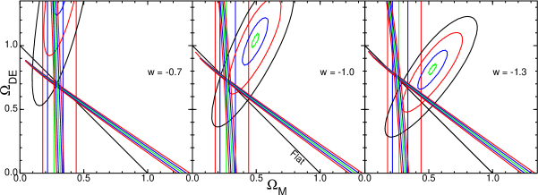
Figure 2: Constraints on the dark energy density and the matter density from four relatively precise cosmological measurements for three different values of the dark energy equation of state. The ellipses show $\Delta\chi^{2}=0.1,\;1,\;4\;\&\;9$ for my fits to the supernova data [29], while the lines show $-2\sigma,\;-1\sigma,\;0,\;1\sigma,\;\&\;2\sigma$ values for $H_{\circ}$ [33] (vertical), baryonic oscillations in the SDSS [34] (not quite vertical), and the CMB acoustic peak angular scale [27] (inclined). The concordance at $w=-1$ is gradually lost for other values of $w$.

The current cosmological literature is again seeking two numbers, but a different set of two numbers. These are the equation of state parameter $w=P/\rho c^{2}$ and its time derivative $w^{\prime}$. $w$ is exactly $-1$ for a cosmological constant, but will be different for models involving evolving scalar fields. If $w$ is not exactly $-1$ then it will interact with matter fluctuations via gravity, and thus the dark energy will be a function of both space and time or redshift. But since the Universe is almost homogeneous and isotropic, the average of $w$ and $w^{\prime}$ over space should be a good description of the evolution of dark energy.

However, there is a very strong tendency among theorists to assume the Universe is flat when seeking $w$ and $w^{\prime}$. This is a logical error, since the evidence for a flat Universe comes from the agreement of the concordance $\Lambda$CDM model with all the data. But the concordance $\Lambda$CDM model has $w=-1$ and $w^{\prime}=0$ exactly. If $w$ and $w^{\prime}$ are allowed to vary, then the evidence for a flat Universe must be re-evaluated. Limits on $w$ and $w^{\prime}$ are only valid when a simultaneous fit for all relevant parameters is done. And when fitting to the CMB data, the spatial variations in the dark energy density should be included even though they are O$(10^{-5})$, since the CMB $\Delta T/T$ is of the same order.

9 Discussion

The progress in cosmology over the past century has been astronomical. We have gone from one fact in 1905 to hundreds of observed facts in 2005.

In terms of the mass of the known Universe the progress is even greater. In 1905 Kapteyn might have given the mass of the Universe as $10^{9}\;M_{\odot}$. Today the mass of the Universe is much larger than the mass of the Hubble volume $M=(4\pi/3)\rho_{crit}(c/H_{\circ})^{3}=0.5c^{3}/(GH_{\circ})=4.4\times 10^{22}\;M_{\odot}$ so we can claim to have discovered more than 44 trillion times more of the Universe than was known in 1905. But we have also found that 95% of the density of the Universe is mysterious dark matter or dark energy.

Cosmologists today are working on problems that could hardly have been defined in 1905, but they are fortunate in having a large and growing body of precise observations with which to test their speculative constructs. Further observations of the CMB, large scale supernovae surveys, weak lensing and baryon oscillations will all provide major new datasets in the next century, and future progress in cosmology is assured.

References

- (1) J. Kapteyn, 1914, JRASC, 8, 145.
- (2) M. Longair, 1993, QJRAS, 34, 157.
- (3) F. Hoyle, 1948, MNRAS, 108, 372.
- (4) H. Bondi and T. Gold, 1948, MNRAS, 108, 252.
- (5) G. Gamow, 1948, Physical Review, 74, 505.
- (6) R. Alpher and R. Hermann, 1949, Physical Review, 75, 1089.
- (7) A. Einstein, 1917, Sitzung Derichte per Preussischen Akad. d. Wiss., 1917, 142,
- (8) E. Hubble, 1929, PNAS, 15, 168.
- (9) W. de Sitter, 1917, MNRAS, 78, 3.
- (10) A. Friedmann, 1922, Zeitschrift für Physik, 21, 326.
- (11) W. Adams, 1941, ApJ, 93, 11.
- (12) G. Herzberg, 1950, “Spectra of Diatomic Molecules”, (New York: Van Nostrand Reinhold)
- (13) F. Hoyle, 1950, The Observatory, 70, 194-197.
- (14) R. Dicke, R. Behringer, R. Kyhl & A. Vane, 1946, Physical Review, 70, 340-348.
- (15) F. Hoyle & R. Tayler, 1964, Nature, 203 1108.
- (16) R. Sachs and A. Wolfe, 1967, ApJ, 147, 73.
- (17) E. Conklin, 1969, Nature, 222, 971-972.
- (18) P. Henry, 1971, 231, 516.
- (19) P. Peebles, 1971, “Physical Cosmology”, (Princeton: Princeton University Press)
- (20) G. Smoot, Gorenstein, M. & R. Muller, 1977, PRL, 39, 898.
- (21) G. Smoot et al., 1992, ApJL, 396, L1.
- (22) E. Wright et al., 1992, ApJL, 396, L13.
- (23) P. Peebles, 1982, ApJ, 263, L1-L5.
- (24) J. Bond & G. Efstathiou, 1987, MNRAS, 226, 655-687.
- (25) D. Scott, J. Silk, & M. White, 1995, Science, 268, 829-835.
- (26) C. Bennett et al., 1993, ApJS, 148, 1.
- (27) L. Page et al., 2003, ApJS, 148, 233.
- (28) M. Phillips, 1993, ApJL, 413, L105-L108.
- (29) A. Riess et al., 2004, ApJ, 607, 665-687.
- (30) S. Perlmutter et al., 1999, ApJ, 517, 565-586.
- (31) E. Wright, 2002, astro-ph/0201196.
- (32) A. Sandage, 1970, Physics Today, 23, 34.
- (33) W. Freedman et al., 2001, ApJ, 553, 47-72.
- (34) D. Eisenstein et al., 2005, ApJ, 633, 560.