Does Sgr A* Have an Event Horizon or an Intrinsic Magnetic Moment?

Abstract

In previous work we have presented evidence for the existence of intrinsic magnetic moments in black hole candidates. We later developed a general relativistic, magnetospheric eternally collapsing object (MECO) model for black hole candidates and showed that the model is consistent with broad band spectral and luminosity characteristics and accounts for the radio/x-ray luminosity correlations of both galactic black hole candidates (GBHC) and active galactic nuclei (AGN). Since magnetic moments are forbidden attributes for black holes, the MECO model has the potential to test whether black hole candidates are actual black holes. We show here that the MECO model has the advantage of being able to: a) satisfy the luminosity constraints that have been claimed as proof of an event horizon for Sgr A*, b) reconcile the low bolometric luminosity with the expected Bondi accretion rate for Sgr A* by means of a magnetic propeller driven outflow, c) account for the Sgr A* NIR and x-ray luminosities, the general characteristics of its broad band spectrum, and the sequence of flares in different spectral ranges as well as the pattern of its observed orthogonal polarizations. We also include specific predictions for images that may be obtained in sub-millimeter to NIR wavelengths in the near future. High resolution images in radio frequencies should be elongated in an equatorial outflow plane, while high resolution images in shorter infrared wavelengths should be elongated along an orthogonal, magnetic polar inflow axis (generally N-S). Since the emissions in these shorter wavelengths are confined to a narrow axial inflow cone, and radio frequencies are generated primarily at greater distances in the equatorial outflow, there would be no uniform background to provide a silhouette image of a dark central object. Additional future tests for the presence of an intrinsic magnetic moment for Sgr A* will require global solutions for electron density and magnetic field distributions in a Bondi accretion flow into a compact, rotating magnetic dipole. These will provide for definitive tests in the form of detailed calculations of spectral and spatial luminosity distributions and polarization maps for direct comparison with high resolution images of Sgr A*.

Key words: accretion, accretion disks–black hole physics–Galaxy : center–gravitation–infrared: general–magnetic fields

1 Introduction

The existence of black holes is accepted as a fact of the cosmos by many astrophysicists. The evidence for the existence of massive objects that may be compact enough to be black holes is strong, however there is as yet no direct evidence of any mass that is contained within its Schwarzschild radius and even that would not necessarily prove the object to be a black hole. Supermassive compact objects have been found in the nuclei of most galaxies and objects of stellar mass are abundant within our own and other galaxies. While these compact objects are commonly called black holes no compelling observational evidence of an event horizon, the quintessential feature of a black hole, has yet been found. It has been pointed out previously (Abramowicz, Kluzniak & Lasota 2002) that it would be very difficult to prove the existence of event horizons if objects with large surface gravitational redshift exist. Extreme redshifts could make such objects nearly as dark as a black hole (see Appendix A). If not different from a black hole in some other way, it would not seem to matter much whether or not the black hole candidates are actual black holes. On the other hand, nearly every object of stellar mass or greater is known to be magnetic to some degree. Whatever their origins, magnetic fields and their synchrotron radiations are ubiquitous among the black hole candidates. Instead of possessing event horizons, some of these compact objects might be found to be both intrinsically magnetic and highly redshifted. Since magnetic moments are forbidden attributes for black holes, there would be important consequences for astrophysics if some of the black hole candidates were found to possess them. Already some evidence for the existence of magnetic moments has been presented for both GBHC and AGN (Robertson & Leiter 2002, 2004, 2006 Schild, Leiter & Robertson 2006, 2008). Others have reported evidence for very strong magnetic fields in GBHC, e.g., a field in excess of $10^{8}$ G has been found at the base of the jets of GRS 1915+105 (Gliozzi, Bodo & Ghisellini 1999, Vadawale, Rao & Chakrabarti 2001).

These findings provided motivation for the development of a fully general relativistic model of a gravitationally compact, intrinsically magnetic, eternally collapsing object that we call a MECO (Leiter & Robertson 2003, Mitra 2006a,b,c, Robertson & Leiter 2003, 2004, 2006, hereafter RL03, RL04, RL06). A MECO avoids rapid collapse to a black hole state by radiating away its mass-energy at an Eddington limit rate. It is characterized by both an extreme redshift and a strong intrinsic magnetic moment (see Appendix A - D). The large redshift accounts for the low quiescent surface luminosities of GBHC and AGN and their extremely long (many Hubble times) radiative lifetimes. The MECO model has been shown (McClintock, Narayan & Rybicki 2004) to be consistent with the lower limit on the quiescent emission from the GBHC XTE J1118+480. We show here that it is also consistent with the low luminosity of Sgr A*.

The MECO model for disk accreting GBHC and AGN accounts for the existence of their low/hard and high/soft x-ray spectral states. The rotating magnetic moments provide a robust universal magnetic propeller mechanism for spectral state switches (Ilarianov & Sunyaev 1975, Campana et al., 1998, 2002, RL02, RL03). The high/soft $\rightarrow$ low/hard transition marks the start of a magnetic propeller regime, the end of accreting plasma being able to penetrate inside the corotation radius and the beginning of a low state jet outflow. The MECO model correctly predicts (RL04) that this transition occurs at about $\sim 0.02$ of Eddington limit luminosity for both GBHC and AGN. The luminosities at the transition and in quiescence have permitted the determinations of the magnetic moments and spin rates for MECO-GBHC (RL02, RL06, and Eqs 6 & 10, Table 1). Spectral state switches are common to dwarf novae, the neutron stars and GBHC of low mass x-ray binary systems and AGN. They are signatures of intrinsic magnetism, however they have not yet been accepted as such because it is generally believed that the black hole candidates are actual black holes and cannot possess magnetic moments.

MECO interacting with accretion disks, as shown in RL04, can produce low/hard state jet outflows with correlated radio and x-ray emissions ($L_{R}\propto L_{x}^{2/3}$) in accord with observations (Gallo, Fender & Pooley 2003, Markoff et al. 2003, Falcke, Körding & Markoff 2004, Maccarone, Gallo & Fender 2003). To account for the similar correlations for AGN and neutron star or dwarf nova systems, it was necessary to explore the mass scaling relations for the MECO model (RL04). These MECO mass scaling relationships, including those associated with the magnetic moments and spin rates that have been able to account for the Radio/X-ray luminosity correlations of AGN and GBHC (RL04), are listed in the right hand column of Table 1. It is a remarkable fact that no further adjustments to these MECO mass scaling parameters are needed for the successful application of the MECO model to the case of Sgr A*. They also account for the newly discovered quasar accretion structures (Schild, Leiter & Robertson 2006, 2008) revealed by microlensing observations of the quasars Q0957+561 and Q2237+0305. The observed structures are consistent with the strongly magnetic MECO model but do not accord with standard thin disk models of accretion flows into a black hole. Since even the nearest GBHC are much too small to be resolved in the detail shown by the microlensing techniques which were used in the study of Q0957 and Q2237, Sgr A* is likely the only remaining black hole candidate for which resolved images might reveal whether or not it possesses a magnetic moment. For this reason it is important that it be tested.

Because much of the spectrum of Sgr A* appears to originate in synchrotron-cyclotron radiation, a serious test of the hypothesis that Sgr A* might possess an intrinsic magnetic moment will require global solutions for the magnetic field and electron density distributions for some kind of accretion flow. While this will require future detailed simulations that are beyond the scope of the present work, we show in this paper that analytic methods can be used to give here a good accounting of the physical properties of the radio/NIR and X-ray spectral characteristics, luminosities and polarizations that have been observed for Sgr A*. We find that we must consider Bondi accretion for a quiescent MECO and then show that we can reconcile the observed low luminosity of Sgr A* with the expected Bondi accretion flow rate.

For the discussion to follow and also for the convenience of readers who might wish to relate MECO properties to observations of other objects, we have tabulated a number of useful relations in Table 1. Many of the parameters are given in terms of quiescent x-ray luminosity $L_{q}$, or the luminosity, $L_{c}$, at the transition high/soft $\rightarrow$ low/hard state since these are often measurable quantities. Some new developments, minor corrections and general features for the MECO model are presented in Appendixes A - E.

Table 1: MECO Model Equations

MECO Physical Quantity	Equation	(Scaling, $m$ in $M_{\odot}$)
1.   Surface Redshift - (RL06 2)	$1+z_{s}=5.67\times 10^{7}m^{1/2}$	$m^{1/2}~{}$
2.   Quiescent Surface Luminosity $L_{\infty}$ - (RL06 29)	$L_{\infty}=1.26\times 10^{38}m/(1+z_{s})$ erg/s	$m^{1/2}~{}$
3.   Quiescent Surface Temp $T_{\infty}$ - (RL06 31)	$T_{\infty}=2.3\times 10^{7}/[m(1+z_{s})]^{1/4}=2.65\times 10^{5}m^{-3/8}$ K	$m^{-3/8}$
4.   Photosphere Temp. $T_{p}$	$T_{p}=4.9\times 10^{8}m^{-0.032}$ K	$m^{-0.032}$
5.   Photosphere redshift $z_{p}$	$1+z_{p}=1840m^{0.343}$	$m^{0.343}$
6.   GBHC Rotation Rate, units $10^{2}~{}Hz$ - (RL06 47)	$\nu_{2}=0.89[L_{q,32}/m]^{0.763}/L_{c,36}~{}\approx 0.6/m~{}Hz$	$m^{-1}~{}$
7.   GBHC Quiescent Lum., units $10^{32}~{}erg/s$ - (RL06 45, 46)	$L_{q,32}=1.17[\nu_{2}L_{c,36}]^{1.31}=4.8\times 10^{-3}\mu_{27}^{2.62}\nu_{2}^{5.24}m^{-0.31}$ erg/s	$m$
8.   Co-rotation Radius - (RL06 40)	$R_{c}=7\times 10^{6}[m/\nu_{2}^{2}]^{1/3}$ cm	$m$
9.   Low State Luminosity at $R_{c}$, units $10^{36}~{}erg/s$ (RL06 41)	$L_{c,36}=0.015\mu_{27,\infty}^{2}\nu_{2}^{3}/m$  erg/s	$m$
10.  Magnetic Moment, units $10^{27}~{}G~{}cm^{3}$ - (RL06 41, 47)	$\mu_{27,\infty}=8.16[L_{c,36}m/\nu_{2}^{3}]^{1/2}~{}~{}~{}\mu=1.7\times 10^{28}m^{5/2}~{}~{}~{}G~{}cm^{3}$	$m^{5/2}~{}$
11.  Disk Accr. Magnetosphere Radius - (RL06 38)	$r_{m}(disc)=8\times 10^{6}[\mu_{27,\infty}^{4}/(m\dot{m}_{15}^{2})]^{1/7}$ cm	$m$
12.  Spherical Accr. Magnetosphere Radius	$r_{m}(sp)$ or axial $z_{m}(in)=2.3\times 10^{7}[\mu_{27,\infty}^{4}/(m\dot{m}_{15}^{2})]^{1/7}$ cm	$m$
13.  Spher. Accr. Eq. Mag. Rad. Rotating Dipole (RTTL03)	$r_{m}(out)=1.2\times 10^{7}[\mu_{27}^{2}/(\dot{m}_{15}\nu_{2})]^{1/5}$ cm	$m$
14.  Equator Poloid. Mag. Field - (RL06 41, 47, $B_{\perp}=\mu_{\infty}/r^{3}$)	$B_{\infty,10}=250m^{-3}(R_{g}/r)^{3}[L_{c,36}/(m^{5}\nu_{2}^{3})]^{1/2}$ gauss	$m^{-1/2}$
15.  Low State Jet Radio Luminosity - (RL04 18, 19)	$L_{radio,36}=10^{-6.64}m^{0.84}L_{x,36}^{2/3}[1-(L_{x,36}/L_{c,36})^{1/3}]$ erg/s	$m^{3/2}$

2 Sgr A*

Perhaps the strongest claimed evidence for an event horizon in any black hole candidate is the one made for Sgr A* (Broderick and Narayan 2006, hereafter BN06) based on its low radiated flux in the near infrared. The bolometric luminosity ($\sim 10^{36}~{}erg/s$) and x-ray luminosity ($\sim 2\times 10^{33}~{}erg/s$) of Sgr A* are also far lower than expected (Baganoff et. al., 2003) from the standard thin accretion disk model used for x-ray binaries and quasars. The bolometric luminosity is only about $2\times 10^{-9}$ of the Newtonian Eddington limit rate for an object of $3.7\times 10^{6}M_{\odot}$. Nevertheless, if the bolometric luminosity originated from accretion to a hard surface, with 100% efficiency, it would require an accretion rate of no less than $10^{15}~{}g/s$ ($2\times 10^{-11}M_{\odot}/yr$). BN06 considered surface thermal radiations from an object with radius in the range $2R_{g}<R<100R_{g}$, where $R_{g}=GM/c^{2}\approx 5.5\times 10^{11}~{}cm$ for a mass of $\sim 3.7\times 10^{6}M_{\odot}$. Subject to three critical assumptions they showed that if redshifted, hard surface thermal emissions at $3.8\mu m$ were produced from such an accretion rate the radiated flux would be too high unless the source radius were larger than about $40R_{g}$. But since the $3.5~{}mm$ emissions of the compact radio source apparently originate within $\sim 10-20R_{g}$ of the central object (Shen et al. 2005, Bower et al. 2004), one would expect the NIR to originate within the same region. It is possible that future VLBI measurements will further constrain the size of the emitting region. The smaller the region, the more severe the constraint on thermal emissions from the mass accretion rate. If confined to the Schwarzschild diameter, the accretion rate in accord with the assumptions of BN06 would have to be less than about $3\times 10^{13}~{}g/s~{}(5\times 10^{-13}M_{\odot}/yr)$.

The assumptions on which these calculations for Sgr A* were based are as follows: (1) A hard surface, possibly highly redshifted, ( $2R_{g}<R<100R_{g}$) assumed to exist within Sgr A*, must radiate in equilibrium with the accreting matter; i.e., the energy transported to this redshifted hard surface by the accreting matter must be radiated immediately with some nonzero efficiency and must escape. (2) In addition the redshifted hard surface assumed to exist in Sgr A* must radiate thermally at a temperature in equilibrium with the rate of energy accretion and (3) General Relativity is an appropriate description of gravity external to the surface. BN06 stated that the current NIR flux density measurements already conclusively imply the existence of an event horizon for Sgr A*. Their conclusion is premature, however, because it does not rule out the MECO model. Their assumption of the existence of a hard surface does not apply to the MECO.

The MECO is blanketed by an optically thick pair atmosphere that offers little impediment to accreting baryonic matter. Only about $10^{-10}$ of accreting particle energy can be absorbed by coulomb collisions with electrons or positrons in the pair atmosphere. Collisions with photons in the pair atmosphere are somewhat more effective at absorbing energy. About $10^{-7}$ of plasma accretion energy can be absorbed by collisions of accreting electrons with photons, however, only about one in $10^{10}$ of these compton enhanced photons can get out through the extremely small general relativistic escape cone (see Appendix A - D). The pair atmosphere is essentially a phase transition region. The temperature is buffered near the pair production threshold of $\sim 6\times 10^{9}$ K. Adding energy creates more pairs, but doesn’t raise the temperature. As a result of these considerations, it is apparent that the MECO surface will remain quiescent until accretion pressure would be a significant fraction of the local radiation pressure. For the photosphere temperature of $3\times 10^{8}$ K (Appendix C, Eq. 26) for a MECO model of Sgr A*, the local radiation pressure would be $\sim 2\times 10^{19}$ erg cm^-3 (see Appendix D). At an accretion rate of $\sim 10^{17}$ g/s, (see below) the maximum pressure accreting protons could contribute if all of their momentum were stopped dead right at the photosphere would only be about $10^{-6}$ of the radiation pressure already present there. Since only about $10^{-7}$ of the momentum is transferred to the entire pair atmosphere, it should be quite clear that that the photosphere surface would remain quiescent for this low accretion rate.

For a quiescent MECO, the observed radiated flux at frequency $\nu_{\infty}$ and distance R ( $>3R_{g}$) from the MECO is given by (See Appendix A, Eq. 17)

$$F_{\nu_{\infty}}=\frac{2\pi h\nu_{\infty}^{3}}{c^{2}}\frac{1}{e^{(h\nu_{\infty}/kT_{\infty})}-1}\frac{27R_{g}^{2}}{R^{2}}$$ (1)

With mass $m\approx 3.7\times 10^{6}~{}M_{\odot}$, Eq. 1, Table 1 gives a surface redshift of $z_{s}=1.1\times 10^{11}$. Eq. 2, Table 1 shows that the bolometric luminosity from a MECO of this mass would be about $4.3\times 10^{33}$ erg/s. From Eq. 3, Table 1, its distantly observed temperature would be $T_{\infty}=910~{}K$ with a spectral peak at $3.2\mu m$. For the most constraining (BN06) NIR wavelength of $3.8\mu m$, and the mass and $8~{}kpc$ distance of Sgr A*, the quiescent MECO flux density given by Eq. 1 is 0.47 mJy, which lies below the observational upper limit by a factor of three. Hence the general relativistic MECO model for Sgr A* shows that a black hole with an event horizon is not required in order to be consistent with the low luminosity observational constraints of Sgr A*. But the constraint might also apply to flows that produce external luminosity close enough to the central object. For any model of the accretion process to satisfy the constraint, whatever the nature of the central object, it is necessary to limit the external accretion rate that gets within a few $R_{g}$ of the object.

3 Origins of Observed Radiations

The multiwavelength spectrum of Sgr A* shows (e.g. An et al. 2005) a relatively flat radio spectrum with a flux density dropping steeply from a few $Jy$ at a few hundred $GHz$ to a few $mJy$ in the NIR. The flat radio spectrum has been attributed to compact relativistic plasma within a few $R_{g}$ of Sgr A*. The similar flat radio spectra for GBHC are thought to arise from a jet outflow (Markoff, Falcke & Fender 2001, Falcke, Körding & Markoff 2003). It has been suggested that there could be a small jet outflow from Sgr A* (Falcke & Markoff 2000, Yuan, Markoff & Falcke 2002) but this is certainly not yet a consensus view. In GBHC systems low state GBHC jets have been resolved (Stirling et al. 2001) and studied over a wide range of GBHC luminosity variation (Corbel et al. 2000, 2003). It has further been shown (RL04, Heinz & Sunyaev 2003) that the radio spectra are consistent with mass scale invariant jets. Whether all (e.g., Heinz & Sunyaev 2003), or only part (RL04), of the low state x-ray emissions of GBHC originate in the base of the jet, it is clear that the base of a jet can contribute.

The quiescent radiation from a MECO model for Sgr A* probably would not originate in a jet outflow from an accretion disk. Although more luminous AGN, modeled as MECO, are largely scaled up versions of disk accreting GBHC, there are differences in quiescence. In true quiescence for the MECO-GBHC the inner disk radius lies beyond the light cylinder. But $T_{\infty}\approx 10^{5}~{}K$ for a central MECO-GBHC is much higher than for an AGN. Even for a faint quiescent MECO-GBHC there would be a thermal radiation flux capable of ionizing and ablating the inner regions of an accretion disk out to $\sim 5\times 10^{3}R_{g}$. Ablated material at low accretion rate would fall in and then be swept out by the rotating magnetic field. This would produce the stochastic power-law soft x-ray emissions in the MECO-GBHC quiescent state. For Sgr A*, there would be only the cooler NIR radiation and insufficient luminosity to ablate an inner disk with radius beyond its light cylinder, hence nothing to keep the inner disk further away. If the luminosity of the true quiescent state for Sgr A* would correspond to a disk with inner radius at the light cylinder, it would be at least $L_{q,max}=(2.7\times 10^{30}erg/s)\mu_{27}^{2}\nu_{2}^{9/2}m^{1/2}\sim 3\times 10^{38}~{}erg/s$ (see RL06 Eq. 43 and Table 1 for magnetic moment and spin). But since the luminosity of Sgr A* is well below this level, we can conclude that its luminosity does not arise from a conventional optically thick, geometrically thin accretion disk that extends in to the light cylinder. This leaves a Bondi accretion flow as the likely spectral source for a MECO model for Sgr A*.

3.1 Bondi Accretion and Magnetic Propeller Effects

It is expected that Sgr A* would accrete plasma in its vicinity via a Bondi capture process. Based on plasma conditions within the central parsec of the galaxy, an accretion rate of $\dot{m}=3\times 10^{-6}M_{\odot}/yr=2\times 10^{20}~{}g/s$ and sound speed of $c_{s,\infty}=550~{}km/s$ have been estimated (Baganoff et al. 2003). The corresponding Bondi radius is $R_{B}=GM/c_{\infty}^{2}=1.6\times 10^{17}~{}cm$. The expected accretion rate creates an interesting conundrum. Even without any surface contributions an accretion flow this large should create far more luminosity than is observed even if it flowed into a central black hole. As shown by Agol (2000), the strong polarization in the radio spectrum of Sgr A* would further constrain the rate of accretion of a magnetically equipartition plasma to be less than about $10^{-9}M_{\odot}~{}/yr$.

It is well known that stellar magnetic fields can severely inhibit accretion to stellar surfaces (e.g., Toropina et al. 2003). “Magnetic propeller effects” associated with stellar rotation (Romanova et al. 2003, hereafter RTTL03, 2005) can cause additional reductions. Revealing animations of these processes can be viewed at
http://astrosun2.astro.cornell.edu/us-rus/$~{}~{}.~{}~{}$Results displayed in Figure 6 of RTTL03 for the “propeller flow regime” show that there is a converging dense accretion flow to the magnetic poles and a very low density, high speed toroidal equatorial outflow. Significant accretion density variations occur in the polar regions within a few times the object radius. The conical flow into the polar regions provides a plausible compact source of some luminosity from within a few $R_{g}$ of the central object while the low density outflow would serve as the source of most of the flat spectrum radio luminosity. The matter flowing in on field lines that enter the polar regions can accrete to the surface, but the bulk of the inflowing mass is ejected in the magnetic propeller regime. RTTL03 demonstrated that as little as 2% of the accreting material could reach the central star in their simulations. An even smaller fraction should reach a more compact central MECO with its much stronger magnetic field.

The propeller flow regime occurs if the magnetosphere radius lies between the corotation and light cylinder radii. MECO co-rotation and light cylinder radii are determined by the mass and spin frequency for both GBHC and AGN (RL02, RL03, RL04, RL06), and respectively, have the same range of values given by $\sim 50-100~{}Rg$ and $500-1000~{}Rg$. As noted by RTTL03, plasma within the magnetosphere corotates with the central object, but only the fraction that penetrates within the corotation radius can accrete to the surface. Figure 7 of RTTL03 shows that beyond the corotation radius, magnetic, centrifugal and pressure gradient forces each exceed the gravitational force and combine to accelerate the equatorial outflow to escape speed.

For the mass of Sgr A* ($3.7\times 10^{6}M_{\odot}$), we expect a spin frequency of $\nu=1.6\times 10^{-5}$ Hz (Table 1, Eq. 6), and a corotation radius of $r_{c}=3.65\times 10^{13}~{}cm=65R_{g}$ (Table 1, Eq. 8). The magnetic moment would be $\mu=4.5\times 10^{44}~{}Gcm^{3}$ (Table 1, Eq. 10). As shown by RTTL03, the Alfven surface in a Bondi flow has a complex shape. The axial and equatorial magnetospheric radii are unequal. RTTL03 showed good agreement between the equatorial magnetosphere radius of their simulation and the radius calculated from Eq. 13 Table 1, for which the outflow is assumed to occur over about 30% of the $4\pi$ solid angle surrounding the dipole. The equatorial radius is determined by equating the energy density of the magnetic field to the kinetic energy density of matter thrown from the equatorial magnetosphere. The equatorial magnetosphere radius for an accretion rate of $3\times 10^{6}M_{\odot}/~{}~{}yr$ would be $r_{m}(out)=2.7\times 10^{14}~{}cm\sim 500R_{g}$ (Table 1 Eq. 13), which is not far inside the light cylinder radius of $3\times 10^{14}~{}cm$. It should be noted that the equatorial magnetic field strength is still $\sim 20~{}-~{}40~{}~{}G$ in the region between magnetosphere and corotation radii, but the kinetic energy density of departing plasma is sufficient to drag the magnetic field lines along with the outflow. In the outflow regions nearer the corotation radius it can be seen in Figure 1 that much of the flow is also loaded onto outward trending portions of the magnetic field lines. The polar magnetosphere radius is determined by the same balance of kinetic energy density and magnetic field energy density along the dipole axis. Since the incoming flow merely attaches to field lines having essentially the same direction, no axial magnetospheric shock is expected. The polar axial magnetosphere radius would be $z_{m}(in)=10^{15}~{}cm\sim 1800R_{g}$ (Table 1, Eq. 12). With the corotation radius well within the magnetosphere radius a MECO model for Sgr A* would be in a strong propeller regime.

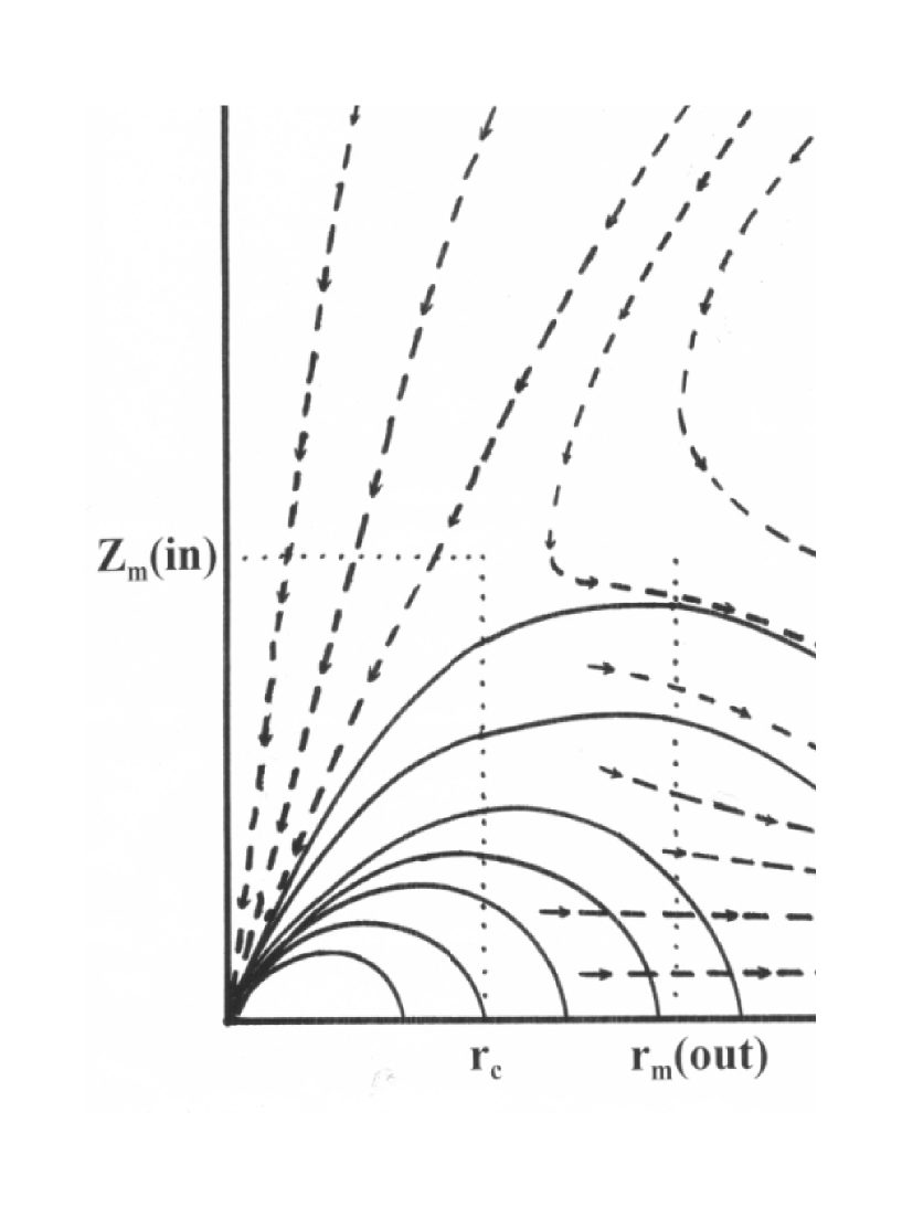
Figure 1: Schematic diagram of accretion flow into a rotating magnetic dipole. Solid lines are magnetic field lines, dashed lines with arrows indicate flow lines. Dotted lines mark corotation and magnetosphere radii. The part of the flow that reaches the axial Alfven surface at $z_{m}(in)$ and continues to the MECO surface is approximately conical.

For a plasma flow to reach a rotating central dipole aligned along the z-axis, it must enter inside the corotation radius. This can occur easily for plasma flowing into the polar regions of the magnetosphere. This part of the flow takes place in a spherically symmetric conical pattern while the pattern elsewhere is a circulating mix of inflow and outflow. A schematic diagram of the flow is shown in Figure 1. The part of the flow that can reach the central dipole enters at the top and bottom of a cylindrical volume whose flat circular ends have a radius equal to the corotation radius and whose height extends the axial magnetosphere distance, $z_{m}(in)$ above and below the equatorial plane. The parts of the flow that do not penetrate the corotation radius at $z_{m}(in)$ are eventually ejected in the low density equatorial outflow. The fraction of a Bondi flow that can reach the central dipole is just the fraction of $4\pi$ steradians that is subtended by the circle at distance $z_{m}(in)$. This fraction is $f=2\pi r_{c}^{2}/(4\pi z_{m}(in)^{2})=r_{c}^{2}/(2z_{m}(in)^{2})$. The factor of two in the first numerator is for plasma entering both poles . For $r_{c}=3.65\times 10^{13}~{}cm$ and $z_{m}(in)=10^{15}~{}cm$, we find $f=6.7\times 10^{-4}$. For a Bondi rate of $3\times 10^{-6}M_{\odot}/~{}yr$ only $\sim 2\times 10^{-9}M_{\odot}/~{}yr=1.3\times 10^{17}~{}g/s$ would reach the central MECO.

Since plasma in the outflow cannot have gotten closer than the corotation distance to the central MECO, we do not expect it to contribute to the high frequency NIR spectral components observed for Sgr A*. As described below, these, SSC x-rays and some thermal brehmsstrahlung should be generated in the conical polar inflow. The expanding equatorial outflow would be expected to produce flat spectrum radio emissions similar to those produced by jets. Although some radio emissions would also be produced within the inflow region, the larger amount of outflowing plasma would dominate the radio emissions. Other than the quiescent thermal brehmsstrahlung contributions discussed below, most of the Sgr A* spectrum consists of cyclotron/synchrotron radiations. Of course it is necessary to know the distributions of magnetic field strengths, plasma densities and temperatures before accurate predictions of emission rates associated with the above processes can be calculated. Global density, electron temperature and magnetic field patterns for magnetic propeller flows similar to those of RTTL03 will be needed in the future. Nonetheless we will show in this paper that analytical methods can be used to produce quantitative and qualitative predictions about the observed spectral characteristics that provide a very plausible case for the existence of a highly red-shifted supermassive MECO in the center of Sgr A*.

As described in Appendix E, we have solved the energy equation for spherical flow for application to the axial cones. The characteristics in this part of the flow are determined primarily by conditions at the Bondi radius. This solution clearly does not apply to the more complex flow pattern outside the axial cones. Flow speeds, ion densities and temperatures for the axial flows are shown in Table 2. For a monatomic gas, the flow never becomes supersonic, though it closely approaches sonic speed everywhere in the polar flow within the magnetosphere. The sonic speed is half what the free-fall speed would be. The general character of the flow is such that ion density varies as $n\propto r^{-3/2}$, ion temperature as $T\propto r^{-1}$, flow speed as $v\propto r^{-1/2}$ and electron temperature as $T_{e}\propto r^{-1/2}$. As described and calculated in Appendix E, the electrons gain the bulk of their energy from collisions with ions but do not thermally equilibrate with them. Electron temperatures, axial magnetic field strength, cyclotron frequencies and Larmor radii are shown in Table 2. The Larmor radii are much larger than the mean particle spacing, $n^{-1/3}$ until $r\sim 30R_{g}$ and the flow is optically thick until then. The flow is Compton thin throughout.

For a number of reasons, we have limited calculations in Table 2 to $r\geq 3R_{g}$. First, the energy equation ceases to apply as ion speeds become relativistic and it becomes necessary to distinguish between coordinate speed and physical three-speed in strong gravity. These distinctions do not change the qualitative features obtained by using the energy equation below $30R_{g}$, which is a little beyond its range of exact applicability. Second, the luminosity generated near $3R_{g}$ is so refracted gravitationally that it would appear to come from a larger region. Third, the classical dipole expression for the magnetic field begins to need modification as gravitational redshift becomes significant inside $3R_{g}$ (Appendix B) . Lastly, the gravitational redshift and Lorentz factors reduce the distantly observed cyclotron radiation frequencies by more than the amount that the relativistically enhanced magnetic field increases them. A limiting frequency of a few times $10^{14}~{}Hz$ is approached near $3R_{g}$. In effect, the inflow synchrotron spectrum cuts off below the NIR anyway. This interesting limiting frequency is set by the the magnitude of the MECO surface magnetic field. The magnetic field is constrained to be no larger than would produce bound electron-positron pairs on the MECO baryon surface. For this reason it follows that strength of the MECO magnetic moment is not a free parameter, but rather is a result of a quantum electrodynamic stability constraint on the highly red shifted, Eddington limited collapse process of the MECO suface described by the Einstein-Maxwell equations (see RL06 and Appendix B).

3.2 Spectral Characteristics of the Bondi Flow

The plasma outside the magnetosphere can weakly radiate via thermal brehmsstrahlung and synchrotron processes, but the electrons are generally too cool to produce much luminosity. Inside the magnetosphere strong, ordered magnetic fields exist and cyclotron emission would be dominant until the accreting electrons become mildly relativistic about at the corotation distance. As shown in Table 2, different cyclotron fundamental frequencies are generated in the polar inflow and the equatorial outflow, but both inflow and outflow can contribute throughout most of the radio frequency range to $\sim 10^{12}~{}~{}Hz$. The reason for this is that the mean particle spacing, $n^{-1/3}$ is much smaller than the Larmor radius except in parts of the inflow that get inside $\sim 30R_{g}$. The mean time between collisions, roughly the mean particle spacing divided by the mean electron speed, is $\sim 10^{-12}~{}~{}s$ until a distance of $\sim 30R_{g}$ is reached. Hence collision broadening will spread the cyclotron/synchrotron frequency range to about $10^{12}~{}~{}Hz$ in both inflow and outflow.

For the MECO magnetic moment of $4.5\times 10^{44}~{}G~{}~{}cm^{3}$, the strongest magnetic field that electrons in the outflow could encounter would be $\sim 9200~{}G$ at the corotation distance on the equatorial plane and the highest cyclotron frequency that they would generate would be $26~{}GHz$, however, as explained, the spectrum produced by electrons that eventually depart in the outflow would be collision broadened to as much as $10^{12}~{}~{}Hz$. As the outflow continues outward it rapidly becomes less dense, its emissions less collision broadened and generally of lower frequency. Since the lowest cyclotron frequency generated within the inflow and inside the corotation radius would be the $51~{}~{}GHz$ shown in Table 2, we can say that any lower frequencies would most likely originate in the much larger mass that eventually departs in the equatorial outflow. This picture is consistent with the observation of a flare at $23~{}~{}GHz$ occurring later than the flare at $43~{}GHz$ (Yusef-Zadeh et al. 2008) and thus indicating an outflow with lower frequencies produced further out in the outflow. It would also not be surprising if the major contribution to the earlier corresponding flare observed at $353~{}~{}GHz$ ($850\mu~{}m$) also originated in the outflow, but closer to the corotation boundary distance.

Since the electrons in the outflow cannot get within $30R_{g}$, they can’t contribute to frequencies above $\sim 10^{12}~{}~{}Hz$. Thus we can say that the $10^{12}~{}~{}Hz$ to NIR range would be generated entirely within the conical inflow. In addition, above $10^{12}~{}~{}Hz$, the Larmor radius becomes smaller than the mean particle spacing. The flow thus becomes optically thin inside $25-30R_{g}$, with fundamental cyclotron frequencies dominating the spectrum without significant collision broadening. Hence we see that the morphology of the plasma polar inflow-equatorial outflow, associated with the existence of an intrinsic MECO dipole magnetic field in the center of Sgr A*, presents us with a natural way to associate particular frequencies with different positions on the axis ($\nu\propto B\propto z^{-1/3}$). What is even more interesting is the fact that in context of Bondi accretion onto Sgr A*, the differing spectral ranges of the equatorial outflow and the polar inflow predicted by the MECO model for Sgr A* are in agreement those required in the two spectral component model of Sgr A* proposed by Agol (2000).

3.3 Flares and Timing Considerations

Recent measurements (Yusef-Zadeh et al. 2006, 2008) show that x-ray and NIR flares preceded some corresponding flares observed at radio frequencies. However, if NIR originates entirely in the inflow, it would seem that flares in the radio would also be produced earlier in the inflow at radio frequencies by plasma in transit from greater distances. For example, a flare at $10^{12}~{}Hz$ ($1000~{}GHz$) would be generated in the axial flow field at $\sim 1.4\times 10^{13}~{}~{}cm=25R_{g}$ compared to a distance of $3\times 10^{12}~{}~{}cm=5.5R_{g}$ for a NIR flare at $3\mu m$. At an average flow speed of $\sim 7\times 10^{9}~{}~{}cm/s$ (Table 2), the NIR flare should occur approximately 26 minutes later. Assuming that the flares are caused by variations in the density of material in the Bondi flow, we should actually expect two flares to occur in the radio frequencies. A relatively weak early one should originate in the inflow and a stronger one in the heavier outflow. Differences in flow speed would likely cause them to occur at different times. The inflow is straight down the magnetic field lines at high speed while the plasma in the outflow would be traveling more slowly and changing from inward to outward motion. Its flare would most likely be delayed. As shown in Figure 1 of Yusef-Zadeh et al. (2008) for observations of July 17, 2006 a weak flare at $850\mu m~{}(353~{}~{}GHz)$ preceded an x-ray flare by about half and hour, which was then followed about 1.4 hours later by another much longer and brighter flare at $850\mu m$. Another observation showed (Yusef-Zadeh et al. 2006, Figure 1b) two NIR flares, each of about one half hour duration and only one flare at $850\mu m$. If the latter is associated with the second NIR flare, then it preceded the NIR by about 38 minutes. No $850\mu m$ measurements are shown beyond the occurrence of the second NIR peak, so we don’t know whether or not a larger radio flare followed. Weak radio flares preceding NIR or X-ray flares would be consistent with the MECO inflow. The larger second radio flare occurring after the NIR/x-ray flares would also be expected. While this picture associated with the MECO model is consistent with the flare observations seen in Sgr A*, similar predictions could also be made in terms of a black hole driven disk-jet model for Sgr A* in which some radio frequencies are generated first in the flow into a hot base of an outflowing jet where NIR and x-ray could be produced. Presumably matter of increasing density could flow into the base of a jet and produce some radio flaring before being expelled. Then there could also be another set of radio flares frequencies produced later further up a jet outflow.

Considering the weakness of the observed $850\mu m$ flares that preceded the observed NIR and X-ray flares, it is conceivable that weak NIR/x-ray flares could be observed without noticeable earlier flaring at radio frequencies in the Bondi inflow. Because of the slower flows near the corotation radius in a magnetic propeller outflow, a NIR/x-ray flare without much of a preceding radio flare could still be produced before any radio flares, thus giving a progression of flares that might all be thought to occur in an outflow. Lastly, depending on the size and location of clumps of matter in the incoming Bondi flow, it would be possible for enhanced density to only occur in the outflow portion and produce radio flaring without producing either x-ray or NIR flares. Although these considerations make it seem plausible that we could have combinations of NIR/x-ray or radio flares without always having both, it seems likely that the strongest NIR/x-ray flares would always be associated with both preceding and trailing radio flares in the MECO model.

Table 2: Bondi Flow Plasma, Magnetic and Spectral Parameters

Axial or Radial Eq. Distance (cm)	$T_{9,ion}$ K	$T_{9,e}$ K	$v_{z}$ (cm/s)	$B_{z}$(G)	$\nu(polar)$	$\nu(out)$	$n(cm^{-3})$	$r_{L}$ (cm)
$1.6\times 10^{17}=R_{B}$	$0.022$	$0.022$					$26$
$10^{16}$	$0.20$	$0.09$	$1.1\times 10^{8}$				$700$
$10^{15}=z_{m}(in)$	$1.8$	$0.29$	$4.4\times 10^{8}$	$0.9$	$2.5$ MHz	$1.25MHz$	$1.9\times 10^{4}$	$747$
$10^{14}\approx r_{m}(out)$ (equatorial)	$18$	$0.93$	$1.5\times 10^{9}$	$900$	$2.5$ GHz	$1.25$ GHz	$6.1\times 10^{5}$	$1.4$
$3.65\times 10^{13}=r_{c}$	$49$	$1.5$	$2.5\times 10^{9}$	$1.8\times 10^{4}$	$51$ GHz	$26$ GHz	$2.8\times 10^{6}$	$0.08$
$1.65\times 10^{13}=30R_{g}$	$109$	$2.3$	$3.8\times 10^{9}$	$2\times 10^{5}$	$560$ GHz		$9.1\times 10^{6}$	$0.01$
$10^{13}$	$180$	$2.9$	$4.9\times 10^{9}$	$8.9\times 10^{5}$	$2.5\times 10^{12}$ Hz		$1.9\times 10^{7}$	$2.7\times 10^{-3}$
$1.65\times 10^{12}=3R_{g}$	$1100$	$7.2$	$1.2\times 10^{10}$	$2\times 10^{8}$	$5.6\times 10^{14}$ Hz		$2.9\times 10^{8}$	$1.3\times 10^{-5}$

3.4 Luminosities

As shown in Appendix E, the luminosity produced in the axial inflows to distance $z$ from the MECO is (Eq. 32)

$$L=4.2\times 10^{41}z^{-1/2}~{}~{}~{}erg/s$$ (2)

For $z=3R_{g}=1.65\times 10^{12}~{}cm$, this yields $L=3.3\times 10^{35}~{}erg/s$. To $30R_{g}$ and $560~{}GHZ$, the luminosity in the polar flow would be $1.0\times 10^{35}~{}erg/sec$. For comparison, the spectrum reported by An et al. (2005) shows a luminosity of $1.7\times 10^{35}~{}erg/s$ to a frequency of 560 GHz. The discrepancy between these results occurs primarily in the lower frequencies. The flux at $10^{12}~{}~{}Hz$ consistent with Eq. 2 is about one order of magnitude below the observed radio spectral trend. This should be expected because most of the radio spectrum would be generated in the outflow, but Eq.2 should be fairly accurate in the NIR which is produced only in the inflow.

At frequencies above about $10^{12}~{}Hz$, the axial flow is optically thin and dominated by cyclotron fundamental frequencies that can be associated with position in the dipole magnetic field; i.e., $\nu\propto B\propto z^{-3}$. Thus inside $30R_{g}$, it is also shown in Appendix E that luminosity varies with frequency along the axial flows such that (Appendix E Eq. 33)

$$dL=2\times 10^{32}\nu^{-5/6}d\nu~{}~{}~{}~{}~{}erg/s$$ (3)

Thus the spectral index in the optically thin IR/NIR would be $-5/6$ for the conical inflow model. The average of four measurements reported in BN06 in the NIR wavelength range from $1.6-4.8\mu m$ is $4.7~{}mJy$. Using a distance to Sgr A* of $8~{}kpc$, the average flux calculated here from Eq. 3 for the same four wavelengths is $5.5~{}mJy$. This result and the variability shown by measurements at the position of Sgr A* strongly suggests that the NIR spectrum originates in a variable accretion flow that is consistent with the MECO model. While the flux calculated here is somewhat larger than the lowest flux used in BN06 to constrain an accretion rate to an assumed hard surface, it should be remembered that variability in the accretion flow would produce opportunities to observe both higher and lower luminosities. It should also be noted that the calculated luminosity is sensitive to the electron temperature, which is poorly constrained. On balance, the agreement between MECO calculated and averaged observed luminosities seems reasonable.

In addition to sensitivity to the electron temperature, the luminosity generated in the inflow depends on the MECO spin rate which then determines the size of the corotation radius ($\propto\nu_{s}^{-2/3}$) and hence the fraction of the Bondi flow that can reach the central MECO. We should expect the spin rate to be influenced by angular momentum transported to the MECO by its accretion environment. Nevertheless, the similar corotation radii ($50-100R_{g}$) of disk accreting GBHC and AGN are necessary for consistency with their mass scale independent radio cutoffs at $\sim 0.02$ of Eddington limit luminosity. Given this mass scale invariant property, it is not surprising that they seem to show little variability in spins that scale as $\nu_{s}\propto m^{-1}$. While we must admit that it is fortuitous that a similarly scaled spin provides reasonable results for the MECO model of Sgr A*, it also suggests that it may have had an accretion history similar to that of other AGN.

For an optically thick slice in the inflow at frequencies below $560~{}GHz$, the cyclotron spectrum would produce luminosity from an axial region of thickness $dz$ that would be proportional to $2\nu^{2}kT_{e}/c^{2}$ times lateral surface area $2\pi r_{c}z/z_{m}dz$. The correlation of frequencies with position, $z$, in the inflow is surely weaker in the broad radio spectral band, but if we still associate $z$ with frequency as $z\propto\nu^{-1/3}$, the luminosity from the band would then be proportional to $\nu^{2-1/3-4/3}d\nu$, hence the spectral index for the optically thick band between $51~{}GHz$ and $560~{}GHz$ would be $1/3$, compared to the reported $0.43$ (An et al. 2005). On the other hand, if viewed looking parallel to the equatorial plane, the luminosity in the outflow could be calculated in the same way in a series of slices of thickness $dz$ with outflow radius proportional to $\nu^{-1/3}$ ($\propto B^{-1/3}$) to obtain the same spectral index. Both radio and NIR spectral indexes are sensitive to the shape of the conical inflow pattern. Dipole magnetic field lines have some curvature that would slightly widen the cone at the top. If the “cone” radius were proportional to $z^{b}$ with $b>1$, it would increase the overall luminosity and spectral index calculated for the NIR and decrease the spectral index in the optically thick region below the spectral peak. This suggests that some refinements of our model might be expected to produce closer agreement with observations but that is a task for another time.

Electrons become mildly relativistic with Lorentz factors of $\gamma_{e}\sim 2-3$ for small $z$. Some x-ray emission would arise from Compton scattering within $\sim 30R_{g}$ in the polar inflow. Electron densities are also large enough in this region to produce some thermal brehmsstrahlung. The calculation of synchrotron self-compton (SSC) contribution can be started by differentiation of Eq. 2 to obtain the luminosity contribution from axial thickness $dz$ as $|dL|=2.2\times 10^{41}z^{-3/2}dz=(dN_{\nu}/dt)E_{\nu}$, where $dN_{\nu}/dt$ is the rate of production of synchrotron photons of average energy $E_{\nu}$ within $dz$. In passing through distance $r=zr_{c}/z_{m}$, on average, these photons will experience $n_{e}\sigma_{T}r$ collisions, where $n_{e}$ is the electron density and $\sigma_{T}$ the Thompson cross-section. The average energy gained per collision would be $2(\gamma_{e}+1)E_{\nu}(kT_{e}/m_{e}c^{2})$. Substituting for $n_{e}$, $T_{e}$ and $r$ as a function of $z$, and integrating over $z$, gives the x-ray self-synchrotron luminosity as

$$L_{SSC}=3.8\times 10^{49}z^{-3/2}~{}~{}~{}~{}~{}erg/s$$ (4)

which provides about $2\times 10^{31}~{}erg/s$ to $3R_{g}$.

For a gaunt factor of $\sim 5$ for small z, thermal brehmsstrahlung contributions can be calculated similarly. The emissivity obtained is $6.2\times 10^{9}z^{-2.75}~{}~{}erg~{}s^{-1}~{}cm^{-3}~{}Hz^{-1}$. Integration over the axial cone volume and all frequencies yields a thermal (primarily x-ray) luminosity of

$$L_{t}=3\times 10^{34}z^{-1/4}~{}~{}~{}~{}~{}erg/s$$ (5)

This provides another $\sim 3\times 10^{31}~{}~{}erg/s$ to $3R_{g}$.

Though both calculated x-ray luminosities might be increased somewhat by considering a flared “cone”, their combined contributions should still fall well below the $2.4\times 10^{33}~{}~{}erg/s$ observed in the 0.5 - 7 keV band (Baganoff et al. 2003). Nevertheless, both depend on the square of electron density which could enhance their contributions to the luminosity in flares relative to synchrotron luminosity. These x-ray luminosity variations in flares would be strongly correlated with the NIR synchrotron luminosity variations and without time delays since both originate in the same population of electrons.

A substantial fraction of the quiescent x-ray luminosity appears to come from a spatially extended source (Baganoff et al. 2003). There is a considerable volume in the MECO magnetosphere in which temperatures and densities would be high enough to produce thermal x-rays. Within the rough bounds of the magnetosphere outside the corotation radius there is a volume of $2\pi r_{m}(out)^{2}z_{m}(in)\sim 3\times 10^{44}~{}~{}cm^{3}$. Using $10^{14}~{}~{}cm$ as an average radius in the Bondi flow, we estimate the corresponding electron temperature to be $10^{9}~{}~{}K$ and the electron density to be $10^{6}~{}~{}cm^{-3}$. For these parameters, a gaunt factor of 3 and the $1.6\times 10^{18}~{}~{}Hz$ bandwidth from 0.5 - 7 keV, we find an average thermal brehmsstrahlung emission rate of $10^{-11}~{}~{}ergs^{-1}cm^{-3}$. Multiplying by the magnetosphere volume, we obtain $\sim 3\times 10^{33}~{}~{}erg/s$, which is reasonably close to the observed quiescent x-ray luminosity of Sgr A*.

The axial inflows constitute such a small fraction of the Bondi accretion rate that their contributions to the spectrum below $52~{}GHZ$ are much smaller than the radiation from the much larger outflow. We don’t know how much the outflows might contribute in harmonic frequencies above $26~{}GHz$, but since the luminosity calculated for the axial flow did not account for the observed luminosity or flux to a frequency of $560~{}GHz$, there is a significant contribution from the outflow that has not been considered. Accurately quantifying the radio luminosity will require knowledge of the plasma and magnetic field distributions, as previously mentioned. All that we can do here is set an upper limit on what might be produced in the outflow. For an accretion rate of $2\times 10^{20}~{}g/s$, electrons would flow outward at a rate of $1.2\times 10^{44}~{}/s$. If they each had the energy they could extract from the protons while reaching the corotation radius, there would be about $2\times 10^{37}~{}erg/s$ available for radiation. The actual radiation rate would probably be much smaller as few of the electrons that would flow out would reach such small distances from the MECO. In this regard, in reaching a steady state, the magnetic propeller eventually must drive the outflow beyond the Bondi radius, cutting off a large fraction of the flow into the Bondi sphere and eventually producing a large torus where the outflow stops beyond the Bondi radius. A luminosity of a few times $10^{36}~{}erg/s$ would seem to be entirely reasonable.

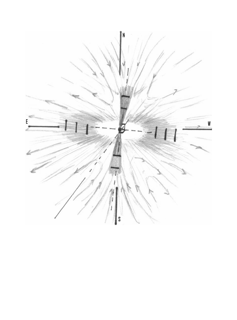
Figure 2: Sketch of Bondi inflow/outflow pattern within the magnetosphere for MECO model of Sgr A*. Most of the radio spectrum to $10^{12}~{}Hz$ is generated in plasma that departs in an equatorial disk-like outflow. The disk outflows are seen limb brightened, generally W-E and E-W as seen against the sky plane. NIR would be produced in the generally N-S and S-N axial inflows. Polarization directions marked with dark bars are essentially perpendicular to magnetic field lines. Quiescent x-ray luminosity would be produced throughout the magnetosphere volume. X-ray SSC and thermal brehmsstrahlung radiation would be produced in flares in the axial inflow NIR region. The luminosity of the central MECO, even at its peak luminosity at $3.2\mu m$, is below observational limits.

3.5 Polarization

The MECO-Bondi flow pattern has two major regions of strong, ordered magnetic fields, with the strongest fields along the polar axis. With the NIR generated within the the polar inflow, its linear polarization direction would be essentially perpendicular to the axis. The equatorial outflow would produce magnetic field lines stretched generally radially along the outflow. These field lines would be perpendicular to the magnetic axis and there are several possibilities for what might be observed, depending on the orientation of the magnetic axis and equatorial plane relative to an observer. Yusef-Zadeh et al. (2006) showed some evidence of outflow from Sgr A*. The apparent flow was in a generally WSW direction from Sgr A*. Proper motion studies have provided confirmation (Muzic et al., 2007) of a general, uncollimated outflow. GRAVITY, a recently proposed high resolution interferometric imaging system (Eisenhauer 2008), should be capable of revealing the nature of the plasma flows in the vicinity of Sgr A* in unprecedented detail. If what has been observed at radio frequencies would be a view into the MECO-Bondi equatorial outflow, we would see the limb brightened regions of the outflow extending WSW (and ENE) against the plane of the sky, with magnetic field lines stretched out along the flow. Linear polarizations from the outflow would then be generally perpendicular to the radio luminosity and in the SSE-NNW direction. A sketch of the way this might appear is shown in Figure 2. The radio polarization has been observed at $230~{}GHz$ (Bower et al. 2003) and clearly displayed, aligned perpendicular to the WSW-ENE direction of the limb brightened part of the outflow. (See Fig. 2.1, http://www.cfa.harvard.edu/sma/newsletter/smaNews_21Dec2006.pdf). Weaker polarization would be produced further out in the flow where the field is weaker and fundamental cyclotron frequencies would be lower.

In addition to the polarization direction at radio frequencies matching expectations for an outflow, strong polarization has been observed in the NIR with a direction roughly 90 degrees (ENE) different from that seen at radio frequencies (Eckart et al. 2008). As noted, this is consistent with the polarization that should be seen perpendicular to the field lines in the inflow if viewed at high inclination to the inflow axis. A view with this orientation would be a view fairly directly into the equatorial outflow and directly down the magnetic field lines of the outflow. Because of the dipole nature of the MECO magnetic field, a view directly into the equatorial plane would have outgoing magnetic field lines on one side of the the plane and ingoing field lines on the other. Outflowing electrons would produce left circular polarization from outflow on one side of the equatorial plane and right circular polarization from the other. Since it is unlikely that the thickness of the outflow would be resolved, there would be a net circular polarization only if viewed at some inclination to the outflow equatorial plane. This could occur while still having a large inclination relative to the inflow axis. Electrons spiraling outward on field lines directed toward us would produce a (negative) left circular polarization. The circular polarization ($\sim 1\%$) of Sgr A* (Bower 2000) is unusually strong for an AGN and approximately double the degree of linear polarization at the same frequency. It seems unlikely that it would originate in a depolarizing medium. While it exhibits short-term variability, it has maintained a stable (negative) sense for over 25 years. In this context it is important to note that the observation of stable directions, with some variability in flares, for both linear and circular polarizations are unique observable features of the MECO model for Sgr A*. All of these properties are determined by the strength of the intrinsic magnetic field of the MECO within the center of Sgr A*.

3.6 Image Appearances

The observed polarizations are consistent with a view close to the equatorial plane of the outflow and across the axial inflow as shown in Figure 2. For this orientation we should see an increasingly wide outflow zone at longer radio wavelengths. Inside any surface of constant magnetic field strength cutting through the outflow, we would expect optically thick cyclotron radiant flux of $j_{\nu}=2\nu^{2}kT_{e}/c^{2}$ to be generated. The apparent size of its limb brightened photosphere image in the equatorial outflow would be roughly proportional to $\nu^{-2}\propto\lambda^{2}$ and ellipsoidal as has been observed (Bower et al. 2004). The major axis of the ellipsoid is apparently aligned with the direction of outflow (Muzic et al. 2007, Yusef-Zadeh et al. 2006, Bower et al. 2004) and perpendicular to the radio polarization direction (Bower et al. 2003). These observations are consistent with our prediction that the apparent size and ellipsoidal shape of the radio images of Sgr A* are due to the equatorial outflow from a MECO in the center of Sgr A*.

Scattering theory also predicts image sizes proportional to $\lambda^{2}$. The image sizes (Bower et al. 2004, Shen et al. 2005) have been interpreted only as scattering features superimposed on a compact object even though the major axis of the observed ellipsoids is twice the length of the minor axis. The galactic center scattering screen is two to three orders of magnitude greater than what is seen in NGC6334B, the next most scattered source (Bower et al. 2004). A heavy screen would be expected for the base of the MECO outflow where its highest radio frequencies would be generated. The claimed detection of an intrinsic size of $48R_{g}$ for Sgr A* rests on apparent deviations from the scattering theory with its wavelength exponent of 2, but for the cyclotron-synchrotron radiations considered here the exponent and deviations at distances inside the corotation radius could arise in a different way. Only much less luminous radio emissions should be generated in the inflow at wavelengths below about 0.3 mm ($10^{12}~{}Hz$). Eq. 33 (Appendix E) gives an expected flux of $0.25~{}Jy$ for this wavelength and a distance of $8~{}kpc$ to Sgr A*.

As shown above, the surface emissions from a MECO model for Sgr A* would peak well below detection limits at $3.2\mu m$. At wavelengths differing by a factor of even two from the thermal peak a MECO would be as dark as a black hole (see Appendix A - C). Since we identify the $10^{12}~{}Hz$ to NIR spectrum as originating in concentrated axial flows into the magnetic poles, we would expect image sizes at optically thin wavelengths to no longer be proportional to $\lambda^{2}$ and to be elongated along the inflow axis rather than the equatorial plane. In the optically thin flow, axial distance from the MECO should be correlated with frequency as $z\propto\nu^{-1/3}\propto\lambda^{1/3}$. Hence on the basis of the MECO model for Sgr A* we are led to the prediction that, if viewed at high inclination to the polar axis, there would be two axial lobes, beginning at about $25R_{g}$ and extending ever closer to a central dark source at shorter wavelengths. Depending on the inclination there might be significant Doppler boosting in the lobe with flow components directed more toward us, however at these radial distances there would not be a uniform background of sub-mm to NIR radiation against which a very dark shadow of the MECO could be viewed. There would be such a background only for wavelengths that originated inside $\sim 5R_{g}$ and were extremely refracted gravitationally. These wavelengths would necessarily be in the NIR.

The MECO-Bondi model presented here can be compared with the radiatively inefficient accretion flow (RIAF) into a black hole (Yuan, Quataert & Narayan 2003). To produce the observed polarization of the optically thick radio emission, the internally generated magnetic field of the RIAF would need to be oriented generally E-W. This might occur in two different ways. (a) If the RIAF magnetic field responsible for the polarization were toroidal within the thick RIAF disk, the RIAF disk would need to be seen nearly edge-on in order to have a consistent magnetic field direction as seen from our side. There would only be one direction of flow observed, either E-W or W-E, in the radio. Accordingly, a suitable radio interferometric array analogous to the proposed NIR GRAVITY array (Eisenhauer et al. 2008) might be able to distinguish a RIAF from a MECO outflow. But in the NIR, the RIAF flow might show no preferential direction as observed with the GRAVITY array because both near and far sides could be seen at once if sufficiently optically thin. The NIR, which would be produced closer to the central black hole is optically thin and would be produced in part by non-thermal electrons. It is the power-law distribution of non-thermal electron energies in the optically thin part of the flow that would produce the orthogonal polarization of the NIR (Agol 2000). (b) If the RIAF magnetic field were poloidal; i.e., with field lines emerging perpendicular to the disk, then the disk would need to be oriented generally N-S, but again seen nearly edge on. Again the flow would appear to be unidirectional. The orthogonal polarization of the NIR would then arise in the same way as before. Thus with either orientation, both polarizations would originate in the geometrically thick disk of the RIAF and it should not look the same as the two zone flow of the MECO-Bondi model shown in Figure 2.

It is clear that the accretion rate in a RIAF must be of order $10^{-9}M_{\odot}~{}/yr$, and far below the Bondi rate of $3\times 10^{-6}M_{\odot}~{}/yr$ in order to produce the observed strong linear polarization within the flow. Exactly how the RIAF might accomplish this is unknown. It has been suggested that the disk evaporates in a wind or that a jet outflow occurs. For a jet outflow to be consistent with observations (Yusef-Zadeh et al. 2006, Muzic et al. 2007, Bower 2003) the RIAF disk would need to be aligned generally N-S with a generally E-W jet. Though this would give more of the appearance of Figure 2, a jet would be an actual collimated outflow rather than just a limb brightened region of a toroidal outflow and the flow in the RIAF disk would still be unidirectional rather than into the central region from both above and below as in the flow into the poles of a MECO. The GRAVITY array should be able to distinguish these possibilities. Ironically, if inflows were observed to disappear into an unseen dark object from both above and below, it could be mistaken for the flow into a black hole event horizon, but some explanation would then be required for an equatorial outflow which ought to also be observed.

4 Summary

We have shown that the MECO model accounts for the lack of observed surface luminosity from Sgr A*. Although it is necessary to know the global distributions of electron density and magnetic fields before spatial and spectral energy distributions can be accurately calculated, we have shown that a spectrum of approximately the correct luminosity and spectral indexes would be produced in the inflow-outflow zones of a Bondi accretion flow into the magnetic field of a MECO. The equatorial outflow would produce optically thick cyclotron radiation with positive spectral index at frequencies below $\sim 1000~{}~{}GHz$. The axial inflow would produce steeply declining (negative index) optically thin NIR emissions as well as some correlated x-ray SSC and brehmsstrahlung emissions that could be observed in flares caused by high density clumps in the inflow. We have shown that timing of flares in radio/NIR/x-ray bands is consistent with the MECO-Bondi model, with some weak sub-mm flaring preceding the strongest NIR and SSC x-ray flares which are then followed by stronger delayed sub-mm and radio flare emissions.

The part of the Bondi flow that eventually departs in the equatorial outflow would produce radio emissions, possibly to frequencies as high as $\sim 1000~{}~{}GHz$, and including nearly everything below $\sim 50~{}~{}GHz$. The bulk of the quiescent x-ray luminosity would be thermally generated within the magnetosphere in a mixed inflow/outflow pattern of $10^{14-15}~{}~{}cm$ size. We have shown that the low bolometric luminosity of Sgr A* can be reconciled with an expected Bondi accretion rate in a completely natural way. The magnetic propeller mechanism is a robust, stable physical mechanism for reducing the Bondi accretion rate to levels compatible with the low luminosity of Sgr A*. The only parameters that have been necessary for these calculations are the ion density and sound speed at the Bondi radius, mass, magnetic moment and spin. The first three of these have been taken from work reported by others. The intrinsic magnetic moment of a MECO is an inherent, mass dependent feature which is generated by the effects of the quantum electrodynamic stablility conditions that are required by the Einstein-Maxwell equations that describe the highly red shifted Eddington limited MECO collapse process (RL06). Its magnitude sets a natural high frequency limit for the synchrotron emissions in the axial inflow. Our estimate of spin has been taken from our previous work that has accounted for the radio/x-ray luminosity correlations and spectral state switches for AGN and GBHC (RL04) and the microlensed image of the quasar Q0957+561 (Schild, Leiter & Robertson 2006). In retrospect, it is fortuitous that this choice has worked out well, but it suggests that the accretion history of Sgr A* may be similar to that of other AGN.

Since they do not possess event horizons, highly red shifted general relativistic MECO contain intrinsic magnetic moments that can interact with their environments. The intrinsic MECO magnetic moment automatically produces the ordered magnetic fields necessary to account for the observed strong linear polarization. In the MECO-Bondi inflow-outflow model for Sgr A* described here, there are regions of differing magnetic field strength and orientation, strong density variations and both inflows and outflows. We have shown that there are places of origin in this flow for all of the spectral, spatial, polarization and timing features that have so far been observed for Sgr A*. The patterns of inflow and outflow differ from those expected of black hole models and should be observable by the proposed GRAVITY array (Eisenhauer et al. 2008). On the basis of the MECO-Bondi model for Sgr A* we predict that high resolution images in radio frequencies should be elongated in the limb brightened outflow zone, while high resolution images in shorter wavelengths should be elongated along an orthogonal polar axis. Since the emissions in these shorter wavelengths are confined to the narrow axial inflow region, there would be no uniform background to provide a silhouette image of a dark MECO except for strong gravitational refraction effects on NIR frequencies generated inside $\sim 5R_{g}$. Everything inside $\sim 25R_{g}$ would just be dark in the radio frequencies.

The qualitative consistency of the MECO-Bondi model provides added incentive for doing additional simulations which, in order to succeed, will require substantial computational facilities and expertise. Calculations of the global magnetic field and density distributions will be necessary first steps before synchrotron emissions in the outflow can be calculated. In order to add spectral details, smaller calculation grids close to the central dipole and consideration of light paths in strong field gravity will be required and could be challenging, even for the original US-Russia supercomputer collaboration that produced the work of RTTL03. Calculations extending into the region near the photon sphere ought to be able to provide spectral and image details that could be compared with the increasingly high resolution images of Sgr A*. Further corroboration of the MECO-Bondi model for Sgr A* could be found if further observations eventually reveal NIR lobes for accretion flow into the magnetic polar regions, though they would likely be smeared into ellipsoids by gravitational refraction. A pattern of expected polarizations of radiation should also be computed. The MECO parameters for spin and magnetic moment used here provide a place to start, but for best comparisons these parameters, as well as the Bondi flow parameters should be varied. Rather detailed calculations of what might be seen for different axis orientations will also be necessary. It is our hope that the present paper will provide motivation for the additional work to be done.

5 Appendix

A. ECO Models

An “eternally collapsing object” ECO is a gravitationally compact mass supported against gravity by internal radiation pressure (Mitra 2006). In its outer layers of mass, a plasma with some baryonic content is supported by a net outward flux of momentum via radiation at the local Eddington limit $L_{Edd}$ given by

$$L_{Edd,s}=\frac{4\pi GMc(1+z_{s})}{\kappa}$$ (6)

Here $\kappa$ is the opacity of the plasma, subscript s refers to the baryonic surface layer and $z_{s}$ is the gravitational redshift at the surface. In General Relativity $z$ is given by

$$1+z=1/\sqrt{1-2GM/c^{2}R}$$ (7)

For a hydrogen plasma, $\kappa=0.4$ cm² /g and

$$L_{Edd,s}=1.26\times 10^{38}m(1+z_{s})~{}~{}~{}~{}erg/s$$ (8)

where $m=M/M_{\odot}$ is the mass in solar units.

Since the temperature at the baryon surface is beyond that of the pair production threshold, there is a pair atmosphere further out that remains opaque. The net outward momentum flux continues onward, but diminished by two effects, time dilation of the rate of photon flow and gravitational redshift of the photons. The escaping luminosity at a location where the redshift is $z$ is thus reduced by the ratio $(1+z)^{2}/(1+z_{s})^{2}$, and the net outflow of luminosity as radiation transits the pair atmosphere and beyond is

$$L_{net~{}out}=\frac{4\pi GMc(1+z)^{2}}{\kappa(1+z_{s})}$$ (9)

Finally, as distantly observed where $z\rightarrow 0$, the luminosity is

$$L_{\infty}=\frac{4\pi GMc}{\kappa(1+z_{s})}$$ (10)

For hydrogen plasma opacity of 0.4 cm² g^-1, and a typical GBHC mass of $7~{}M_{\odot}$ this equation yields $L_{\infty}=8.8\times 10^{38}/(1+z_{s})$ erg s^-1. But since the quiescent luminosity of a GBHC must be less than about $10^{31}$ erg s^-1, we see that it is necessary to have $z_{s}>8.8\times 10^{7}$. Even larger redshifts are needed to satisfy the quiescent luminosity constraints for AGN. This is extraordinary, to say the least, but perhaps no more incredible than the $z=\infty$ of a black hole.

At the low luminosity of Eq. 10, the gravitational collapse is characterized by an extremely long radiative lifetime, $\tau$ (Robertson & Leiter 2003, Mitra 2006) given by:

$$\tau=\frac{\kappa c(1+z_{s})}{4\pi G}=4.5\times 10^{8}(1+z_{s})~{}~{}yr$$ (11)

With the large redshifts that would be necessary for consistency with quiescent luminosity levels of BHC, it is clear why such a slowly collapsing object would be called an “eternally collapsing object” or ECO.

For $(1+z)>\sqrt{3}$, radiation is impeded by passage through a small escape cone such that the fraction of radiation that could escape if isotropically emitted at radius R would only be

$$f=27\frac{R_{g}^{2}}{R^{2}(1+z)^{2}}$$ (12)

For very large $z$, $R\approx 2R_{g}$ and $f=(27/4)(1+z)^{-2}$.

At the outskirts of the pair atmosphere of an ECO the photosphere is reached. Here the temperature and density of pairs has dropped to a level from which photons can depart without further scattering from positrons or electrons. Nevertheless, the redshift is still large enough that their escape cone is small and most photons will not travel far before falling back through the photosphere. If we let the photosphere temperature and redshift be $T_{p}$ and $z_{p}$, respectively, the net escaping luminosity is

$$L=\frac{27R_{g}^{2}4\pi R^{2}\sigma T_{p}^{4}}{R^{2}(1+z_{p})^{2}}=\frac{4\pi GMc(1+z_{p})^{2}}{\kappa(1+z_{s})}$$ (13)

But in the radiation dominated region beyond the photosphere, the temperature and redshift are related by

$$T_{\infty}=\frac{T}{1+z}$$ (14)

where $T_{\infty}$ is the distantly observed radiation temperature. Substituting into the previous equation, we obtain

$$L_{\infty}=(27)4\pi R_{g}^{2}\sigma T_{\infty}^{4}=\frac{4\pi GMc}{\kappa(1+z_{s})}$$ (15)

and, for hydrogen plasma opacity

$$T_{\infty}=\frac{2.3\times 10^{7}}{[m(1+z_{s})]^{1/4}}~{}~{}~{}~{}K$$ (16)

The left equality of Eq. 15 can be written in terms of the distantly observed spectral distribution, for which the radiant flux density at distance R ($>3R_{g}$) and frequency $\nu_{\infty}$ would be

$$F_{\nu_{\infty}}=\frac{2\pi h\nu_{\infty}^{3}}{c^{2}}\frac{1}{e^{(h\nu_{\infty}/kT_{\infty})}-1}\frac{27R_{g}^{2}}{R^{2}}$$ (17)

B. MECO

As previously discussed (RL06), if one naively assumes that the photon support for an ECO originates from purely thermal processes, one quickly finds that the temperature in the baryon surface layer would be orders of magnitude higher than the pair production threshold. The compactness guarantees (Cavaliere & Morrison 1980) that photon-photon collisions would produce numerous electron-positron pairs. Drift currents proportional to ${\bf g\times B}/B^{2}$ reactively generate extreme magnetic fields. We assumed that the baryonic surface field reaches an equipartion level with a surface magnetic field of $\sim 10^{20}$ G (Harding 2003, Zaumen, 1976) that is capable of creating bound electron-positron pairs on the baryon surface. The interior magnetic field in a stellar mass MECO-GBHC is about what would be expected from flux compression during stellar collapse. At the MECO surface radius ($R\approx 2R_{g}$), the ratio of tangential field on the exterior surface to the tangential field just under the MECO surface is given by (RL06)

$$B_{\theta,S^{+}}/B_{\theta,S^{-}}=(1+z_{s})/(2ln(1+z_{s}))$$ (18)

$$~{}~{}~{}~{}~{}~{}~{}~{}~{}~{}=10^{20}~{}G/(B_{in}\sqrt{7M_{\odot}/M})$$

We have previously taken $B_{in}=2.5\times 10^{13}$ gauss as typical of the interior field that can be produced by flux compression during stellar gravitational collapse. Using this value the preceding equation has the solution.

$$1+z_{s}=5.67\times 10^{7}m^{1/2}$$ (19)

The magnetic moment of a MECO would be

$$\mu=1.7\times 10^{28}m^{5/2}~{}~{}~{}~{}~{}~{}G~{}cm^{3}$$ (20)

We have found that this magnetic moment, and the spin rates given by Table 1, Eq. 6 give the MECO model a good correspondence with observations of spectral state switches and the radio luminosities of jets for both GBHC and AGN (RL02, RL03, RL04, RL06).

C. The Photosphere

The photosphere, as a last scattering surface, can be found from the condition that (Kippenhahn & Wiggert 1990)

$$\int_{\infty}^{R_{p}}n_{\pm}\sigma_{T}dl=2/3$$ (21)

where $dl$ is an increment of proper length in the pair atmosphere and $n_{\pm}$ is the combined number density of electrons and positrons along the path. Landau & Lifshitz (1958) show that

$$n_{\pm}=\frac{8\pi}{h^{3}}\int_{0}^{\infty}\frac{p^{2}dp}{\exp{(E/kT)}+1}$$ (22)

where p is the momentum of a particle, $E=\sqrt{p^{2}c^{2}+m_{e}^{2}c^{4}}$, k is Boltzmann’s constant, $h$ is Planck’s constant and $m_{e}$, the mass of an electron. For low temperatures such that $kT<m_{e}c^{2}$ this becomes:

$$n_{\pm}\approx 2(\frac{2\pi m_{e}kT}{h^{2}})^{3/2}\exp{(-m_{e}c^{2}/kT)}$$ (23)

$$~{}~{}~{}~{}~{}~{}~{}~{}~{}~{}=2.25\times 10^{30}(T_{9}/6)^{3/2}\exp{(-6/T_{9})}~{}~{}cm^{-3}$$

where $T_{9}=T/10^{9}$K.

We can express $dl$ in terms of changing redshift as

$$dl=|dr|(1+z)=4R_{g}dz/(1+z)^{2}$$ (24)

for $R\approx 2R_{g}$ Substituting into Eq. 23 and using $T_{\infty}=T/(1+z)$ beyond the photosphere we obtain the relation

$$1.77\times 10^{12}m(T_{\infty,9}/6)\int_{\sqrt{T_{\infty,9}/6}}^{\sqrt{T_{9}/6}}e^{-6/T_{9}}d{\sqrt{T_{9}/6}}=2/3$$ (25)

Using Eqs. 16 and 19, we have numerically integrated this equation to obtain the photosphere temperatures and redshifts for various masses. The results are represented with errors below 1% for $1<m<10^{10}$ solar mass by the relations:

$$T_{p}=4.9\times 10^{8}m^{-0.032}~{}~{}~{}~{}~{}~{}~{}~{}K$$ (26)

and

$$1+z_{p}=1840m^{0.343}$$ (27)

These relations, though little different from those of RL06, correct an error in our previous development of the photosphere temperature.

D. Accretion Efficiency For MECO Surface Luminosity

We need to reconsider how accreting material interacts with a MECO. BN06 assumed that for large redshifts, accretion energy would be converted to luminosity immediately with 100% efficiency. In previous work (RL03, RL06) we mistakenly made the same assumption. It is true that a MECO will eventually achieve 100% efficiency, but the conversion takes place on the time scale of the MECO radiative lifetime. Accreting particles that reach the photosphere do not produce a hard radiative impact. They first encounter soft photons, then photons of $\sim 1$ Mev and electron-positron pairs near the photosphere and they eventually penetrate the baryon surface where the net outflowing luminosity is already at the local Eddington limit rate. This provides a very soft landing.

Perhaps the easiest way to show the difference between landing on a cushion of photons and striking a hard surface is to consider the pressure that accreting matter could exert if stopped dead at the photosphere and compare that to the radiation pressure already there. Radiation pressure at the photosphere (hence the luminosity also) would need to change by only about the same amount as the accretion pressure for the MECO to remain stable.

Consider a particle of rest mass $m_{o}$ in radial free fall from infinity. Its speed as it reaches the photosphere would be essentially light speed, $c$, according to an observer at the photosphere, and it would have a momentum of $\gamma m_{o}c$, where $\gamma=1+z_{p}$ is the Lorentz factor. If particles arrive at the locally observed rate of $dN/dt_{p}$, then the quantity of momentum deposited according to the observer at the photosphere would be $(dN/dt_{p})(1+z_{p})m_{o}c$. With the substitution of $dt/(1+z_{p})$ for $dt_{p}$, this becomes $(dN/dt)m_{o}(1+z_{p})^{2}c$. Thus the rate of momentum transport, as observed at the photosphere is $\dot{m_{\infty}}(1+z_{p})^{2}c$, where $\dot{m_{\infty}}=m_{o}dN/dt$.

If momentum were deposited uniformly at the photosphere, the accretion pressure would be $p_{accr}=\dot{m_{\infty}}(1+z_{p})^{2}c/(4\pi R^{2})=9.2\times 10^{4}\dot{m_{\infty}}m^{-1.314}$ erg cm^-3, using Eq. 27 for $z_{p}$ and $R=2R_{g}$. For the mass of Sgr A* and $\dot{m_{\infty}}=1.3\times 10^{17}$ g/s, this would yield $p_{accr}=2.9\times 10^{13}$ erg cm^-3. The radiation pressure at the photosphere would be $p_{rad}=aT_{p}^{4}/3=1.5\times 10^{20}m^{-0.128}=2.2\times 10^{19}$ erg cm^-3, using Eq. 26. This pressure ratio would be $p_{accr}/p_{rad}=1.3\times 10^{-6}$, however, the actual ratio of accretion and radiation pressures would be smaller yet because the entire momentum is not deposited in a hard surface impact at the photosphere. Only about $10^{-7}$ of the incoming momentum is transferred to the entire pair atmosphere. This is just too little to affect the radiation leaving the photosphere. Finally, we note that in an equipartition magnetic field, the temperature of the pair plasma layer is buffered near the pair threshold temperature. Adding energy just produces more pairs rather than raising the temperature. Of course, for stability, the MECO must adjust its radiation rate to accomodate a growing mass, but as distantly observed, the luminosity produced by the incremental increase of mass is negligible. For mass accretion rate $\dot{m_{\infty}}$ the radiated luminosity increases at a rate of about $(\dot{m_{\infty}}/M)L_{\infty}$. We conclude that the efficiency and thermal equilibrium constraints of BN06 simply do not apply to the MECO surface.

Eventually the radial infall of accreting particles ends, on average somewhere below the MECO baryon surface. With the temperature at the base of the pair atmosphere at $\sim 6\times 10^{9}$ K, Eq. 23 shows the local pair density to be near $10^{30}~{}cm^{-3}$. The proper length thickness of the pair atmosphere is $\sim 7\times 10^{6}~{}cm$ and the optical depth is $\sim 5\times 10^{12}$. Assuming that protons in an accreting plasma interact with the electron-positron pairs via coulomb scattering, the fraction of the accretion energy that they can transfer directly to the pair atmosphere is only $\sim 10^{-10}$. Photons in the pair atmosphere are somewhat more effective in absorbing accretion energy. For conditions in the pair atmosphere, about $10^{-7}$ of the accretion energy can be removed by photon collisions with incoming electrons, however, the escape cone allows only about one in $10^{10}$ of the compton enhanced photons to escape. Most of the brehmsstrahlung produced is therefore buried below the MECO baryon surface which is itself covered by an extremely optically thick layer of pairs for which the escape cone is negligibly small. With due consideration of the small escape cone, it can be easily shown that if accreting protons are stopped in a layer below the photosphere for which the redshift is $z<z_{s}$, then the ratio of accretion pressure to radiation pressure already in the layer is $p_{accr}/p_{rad}=3.6\times 10^{-17}\dot{m}_{\infty}/(m(1+z_{s}))=6.3\times 10^{-25}\dot{m}_{\infty}/m^{3/2}$, for $1+z_{s}=5.67\times 10^{7}m^{1/2}$. Accretion pressure is completely insignificant even for accretion rates exceeding the classical Edddington limit. In effect, a MECO just swallows accreting particles about as effectively as a black hole.

D.1 High/Soft Spectral States
Reconsideration of the MECO surface accretion efficiency necessitates a new interpretation of the high/soft spectral states of disk accreting systems. At accretion rates above the transition to the soft state, most of the luminosity of the high/soft state must arise from the accretion disk rather than the MECO. This can occur with high efficiency corresponding to an accretion disk that can penetrate well inside what would otherwise correspond to the marginally stable orbit of a non-magnetic black hole. The inner disk of a MECO is supported in part by magnetic pressure, as previously described in RL06 and disk accretion efficiencies can reach 42% at the photon sphere at $3R_{g}$. Inside the photon sphere, gravitational redshift offsets the effect on luminosity of additional radiant energy release by accreting matter.

E. Electron Temperatures and Spectral Parameters

The energy equation for the Bondi flow is

$$\frac{v^{2}}{2}+\frac{c_{s}^{2}}{\gamma_{h}-1}-\frac{GM}{r}=const=\frac{c_{s,\infty}}{\gamma_{h}-1}$$ (28)

where $v$ is the bondi flow speed, $\gamma_{h}$ the ratio of specific heats for the gas, $M$ the mass of the central object and $r$ the radial coordinate distance from its center. The continuity equation for a rate of mass flow $\dot{m}$ is

$$\dot{m}=4\pi r^{2}\rho v=const.$$ (29)

We adopt the values $\dot{m}=3\times 10^{-6}~{}M_{\odot}/yr=2\times 10^{20}~{}g/s$, $n_{\infty}=\rho_{\infty}/m_{p}=26~{}cm^{-3}$, $c_{s,\infty}=5.5\times 10^{7}~{}cm/s$ (Baganoff 2003) and a specific heat ratio of $\gamma_{h}=5/3$ for atomic hydrogen. Having adopted these values, they set the Bondi radius as $1.63\times 10^{17}~{}cm$ and they must be entered consistently in the energy equation. We use $c_{s}=\gamma_{h}K\rho^{(\gamma_{h}-1)}$, where $K=p_{\infty}/\rho_{\infty}^{\gamma_{h}}$ for an adiabatic flow. Using $\rho=\dot{m}/(4\pi r^{2}v)$ and substituting into the energy equation produces an equation of the form

$$v^{2}+Av^{-2/3}/r^{4/3}-B-C/r=0$$ (30)

where A, B and C are constants. Solutions for v for various values of r are given in Table 2. Once v has been determined, $\rho$ can be obtained from the continuity equation, and the pressure and proton temperature can be found from the adiabatic conditions. For $\gamma_{h}=5/3$, the inflow never becomes supersonic, but it very closely approaches sound speed (which is half what the free-fall speed would be) by the time the magnetosphere is reached.

For the dilute plasma at the Bondi radius, there is a relatively low frequency of electron-proton collisions. The kinetic energy gained by falling electrons is not sufficient to keep them in thermal equilibrium with the ions. Approximately half of the gravitational energy released goes into heating the ions while the electrons remain relatively cold. The electrons do gain some energy, which we can calculate, in collisions with protons. As the plasma falls by $dr$, the time taken is $dr/v$. An electron travels $v_{e}dt=v_{e}dr/v$ in this time. The number of collisions with ions in this time is the distance travelled divided by the mean free path, $1/n\sigma_{c}$, where $\sigma_{c}=(\pi e^{4}/E_{e}^{2})\ln{\Lambda}$ is the coulomb cross-section. $E_{e}=(3/2)kT_{e}$ is the electron energy, $T_{e}$ the electron temperature and $\ln{\Lambda}$ is the coulomb logarithm, which we assume to have the value 30. For collisions with protons which, on average, have much more momentum than the electrons, the fraction of proton energy, $(1/2)m_{p}v^{2}$, that can be transferred is approximately $2v/v_{e}$. Then while falling dr, an electron gains energy $dE_{e}=(3/2)kdT_{e}=n\sigma_{c}m_{p}v^{2}dr$. Taking $v=(GM/2r)^{1/2}$ for both the proton thermal speed and speed of descent and substituting for $\sigma_{c}~{}(\propto T_{e}^{-2})$ and $n~{}(\propto r^{-3/2})$, this integrates to yield $T_{e}\propto r^{-1/2}$ and specifically,

$$T_{e}=9.3\times 10^{15}r^{-1/2}~{}~{}~{}K$$ (31)

yields the values in Table 2.

An electron moving with the protons at speed $v~{}(=dr/dt)$ in a magnetic field would emit cyclotron radiation at a rate $dE_{R}/dt=2e^{4}v^{2}B^{2}/(3c^{5}m_{e}^{2})$. Comparing this rate for the axial dipole field of a MECO with the mass of Sgr A* with $dE_{e}/dt$ above, we find that the radiation rate would exceed the rate that electron energy is extracted from the protons for $B>8600~{}G$, which holds for $r<5\times 10^{13}~{}cm$, and cyclotron frequencies above $14~{}GHz$. Nearer the MECO at smaller axial distances and higher frequencies, the electron energy extracted from the protons in the flow is essentially all that is available for radiation. This permits a rough calculation of the luminosity generated in the polar inflow. We approximate the polar inflow geometry within the magnetosphere as a cone of lateral radius $a=r_{c}z/z_{m}(in)$ at distance z from the magnetic pole. See Figure 1. The number of electrons in the cone in axial thickness $dz$ is $dN=n\pi a^{2}dz$. Thus the rate that they can radiate is about $dL=dNdE_{e}/dt=n\pi(r_{c}/z_{m}(in))^{2}z^{2}n\sigma_{c}m_{p}v^{3}dz$. Substituting for $n(z)$, $\sigma_{c}(z)$, $v(z),T_{e}(z)$ as before and using $r_{c}=3.65\times 10^{13}~{}cm$, $z_{m}=10^{15}~{}cm$ from equations in Table 1, this reduces to $dL=1.1\times 10^{41}z^{-3/2}dz$, which integrates to give the luminosity for polar inflow to axial distance $z$ as

$$L=4.2\times 10^{41}z^{-1/2}~{}~{}~{}erg/s$$ (32)

This last result includes an additional factor of two to account for inflow into both magnetic poles.

Where the flow is optically thin above $10^{12}~{}Hz$, the Larmor frequency should strongly dominate the spectrum. This frequency is a function of the magnetic field strength, which varies as $r^{-3}$. Alternatively, we can say that position $z$ in the polar axial inflow is correlated with the dominant radiation frequency as $z\propto\nu^{-1/3}$. Substituting $1.36\times 10^{17}\nu^{-1/3}$ for $z$ in the expression just preceding Eq. 32, one obtains

$$dL=2\times 10^{32}\nu^{-5/6}d\nu~{}~{}~{}~{}~{}erg/s$$ (33)

hence the spectral index in the optically thin sub-mm/NIR would be $-0.83$ for the MECO model.

References

- [1] Abramowicz, M., Kluzniak, W. & Lasota, J-P, 2002 A&A, 396, L31
- [2] Agol, E., 2000 ApJ, 538, L121
- [3] An, T., et al., 2003 ApJ, 634,49
- [4] Baganoff, F., et al., 2003 ApJ, 591, 891
- [5] Bower, G., 2000 GCNEWS 11, 4
- [6] Bower, G., et al., 2004 Science, 304, 704
- [7] Broderick, A., & Narayan, R., 2006 ApJ, 638, L21 BN06
- [8] Campana, S. et al., 2002 ApJ 580, 389
- [9] Campana, S. et al., 1998 A&A Rev. 8, 279
- [10] Cavaliere, A. & Morrison, P. 1980 ApJ 238, L63
- [11] Corbel, S., Fender, R.P., Tzioumis, A.K., Nowak, M.A., McIntyre, V., Durouchoux, P.,Sood, R., 2000 A&A 359, 251
- [12] Corbel, S., Nowak, M.A., Fender, R.P., Tzioumis, A.K. Markoff, S., 2003 A&A 400, 1007
- [13] Eckart, A. et al. 2008 A&A, July 8 in press /astro-ph0712.3165
- [14] Eisenhauer, F., et al., 2008 Proc. SPIE Astron. Instr., 22-28 June, Marseille, France, in press astro-ph/0808.0063
- [15] Gallo, E., Fender, R., Pooley, G., 2003 MNRAS, 344, 60
- [16] Falcke, H., Körding, E., Markoff, S., 2004 A&A, 414, 895
- [17] Falcke, H., & Markoff, S., 2000 A&A 362, 113
- [18] Gliozzi, M., Bodo, G. & Ghisellini, G. 1999 MNRAS, 303, L37
- [19] Heinz, S., Sunyaev, R., 2003 MNRAS 343, L59
- [20] Harding, A., 2003, Invited talk at Pulsars, AXPs and SGRs Observed with BeppoSAX and Other Observatories, Marsala, Sicily, Sept. 2002 astro-ph/0304120.
- [21] Ilarianov, A. & Sunyaev, R. 1975 A&A, 39, 185
- [22] Kippenhahn, R. & Weigert, A. 1990 ‘Stellar Structure and Evolution’ Springer-Verlag, Berlin Heidelberg New York
- [23] Landau, L. & Lifshitz, E. 1958 ‘Statistical Physics’, Pergamon Press LTD, London
- [24] Leiter, D., & Robertson, S., 2003 Found. Phys. Lett., 16, 143
- [25] Maccarone, T., Gallo, E., Fender, R. 2003 MNRAS 345, L19
- [26] Markoff, S., Falcke H., & Fender, R. 2001 A&AL, 372, 25
- [27] Markoff, S., Nowak, M., Corbel, S., Fender, R., Falcke, H., 2003 New Astron. Rev. 47, 491
- [28] McClintock, J., Narayan, R., and Rybicki, G., 2004, ApJ, 615, 402
- [29] Mitra, A., 2006 New Astron., 12, 146-160
- [30] Mitra, A., 2006 MNRAS 369, 492
- [31] Mitra, A., 2006 Phys. Rev. D, 74, 034010
- [32] Muzik, K., et al., 2007, Proc. Int’l Astron. Union, 2, 415
- [33] Robertson, S. & Leiter, D. 2002 ApJ, 565, 447 RL02
- [34] Robertson, S., Leiter, D. 2003 ApJ, 596, L203 RL03
- [35] Robertson, S., Leiter, D. 2004 MNRAS, 350, 1391 RL04
- [36] Robertson, S., and Leiter, D. 2006 ‘The Magnetospheric Eternally Collapsing Object (MECO) Model of Galactic Black Hole Candidates and Active Galactic Nuclei’, pp 1-45 (in New Developments in Black Hole Research, ed. P.V.Kreitler, Nova Science Publishers, Inc. ISBN 1-59454-460-3, novapublishers.com) RL06 astro-phys/0602543
- [37] Romanova, M., Toropina, O., Toropin, Y., & Lovelace, R., 2003 ApJ, 588, 400
- [38] Romanova, M., Ustyugova, A.,Koldoba, A., & Lovelace, R., 2005 ApJ, 635, L165
- [39] Schild, R., Leiter, D. & Robertson, S., 2006 AJ, 132, 420
- [40] Schild, R., Leiter, D. & Robertson, S., 2008 AJ, 135, 947
- [41] Shen, Z., et al., 2005 Nature, 438, 62
- [42] Stirling A. M., et al., 2001 MNRAS 327, 1273
- [43] Toropina, O., Romanova, M., Toropin, Y., & Lovelace, R., 2003 ApJ 593, 472
- [44] Vadawale, S., Rao, A. & Chakrabarti, S. 2001 A&A, 372, 793V
- [45] Yuan, F., Markoff, S. & Falcke, H., 2002 A&A, 383, 854
- [46] Yuan, F., Quataert, E., Narayan, R., 2003 ApJ 598, 301
- [47] Yusef-Zadeh et al., 2006, in VI Microquasar Workshop: Microquasars and Beyond, Sept. 18-22, 2007, Como, Italy, astro-ph/0612156
- [48] Yusef-Zadeh et al., 2006 ApJ 650, 189
- [49] Yusef-Zadeh et al., 2008 ApJ, 682, 361
- [50] Zaumen, W. T., 1976 ApJ, 210, 776