Quasars Probing Quasars I: Optically Thick Absorbers Near Luminous Quasars

Abstract

With close pairs of quasars at different redshifts, a background quasar sightline can be used to study a foreground quasar’s environment in absorption. We search 149 moderate resolution background quasar spectra, from Gemini, Keck, the MMT, and the SDSS to survey Lyman Limit Systems (LLSs) and Damped Ly$\alpha$ systems (DLAs) in the vicinity of $1.8<z<4.0$ luminous foreground quasars. A sample of 27 new quasar-absorber pairs is uncovered with column densities, $10^{17.2}~{}{\rm cm}^{-2}<N_{\rm HI}<10^{20.9}{\rm cm}^{-2}$, and transverse (proper) distances of $22~{}h^{-1}{\rm\ kpc}<R<1.7~{}h^{-1}{\rm\ Mpc}$, from the foreground quasars. If they emit isotropically, the implied ionizing photon fluxes are a factor of $\sim 5-8000$ times larger than the ambient extragalactic UV background over this range of distances. The observed probability of intercepting an absorber is very high for small separations: six out of eight projected sightlines with transverse separations $R<150~{}h^{-1}{\rm\ kpc}$ have an absorber coincident with the foreground quasar, of which four have $N_{\rm HI}>10^{19}{\rm cm}^{-2}$. The covering factor of $N_{\rm HI}>10^{19}{\rm cm}^{-2}$ absorbers is thus $\sim 50\%$ (4/8) on these small scales, whereas $\lesssim 2\%$ would have been expected at random. There are many cosmological applications of these new sightlines: they provide laboratories for studying fluorescent Ly$\alpha$ recombination radiation from LLSs, constrain the environments, emission geometry, and radiative histories of quasars, and shed light on the physical nature of LLSs and DLAs.

1. Introduction

Although optically thick absorption line systems, that is the Lyman Limit Systems (LLSs) and damped Lyman-$\alpha$ systems (DLAs), are detected as the strongest absorption lines in quasar spectra, the two types of objects, quasars and absorbers, play rather different roles in the evolution of structure in the Universe. The hard ultraviolet radiation emitted by luminous quasars gives rise to the ambient extragalactic ultraviolet (UV) background (see e.g. Haardt & Madau 1996; Meiksin 2005) responsible for maintaining the low neutral fraction of hydrogen ($\sim 10^{-6}$) in the intergalactic medium (IGM), established during reionization. However, high column density absorbers represent the rare locations where the neutral fractions are much larger. Gas clouds with column densities $\log N_{\rm HI}>17.2$ are optically thick to Lyman continuum ($\tau_{\rm LL}\gtrsim 1$) photons, giving rise to a neutral interior self-shielded from the extragalactic ionizing background. In particular, the damped Ly$\alpha$ systems dominate the neutral gas content of the Universe (Prochaska et al. 2005), which provides the primary reservoir for the star formation which occurred to form the stellar masses of galaxies in the local Universe.

One might expect optically thick absorbers to keep a safe distance from luminous quasars. For a quasar at $z=2.5$ with an $r$-band magnitude of $r=19$, the flux of ionizing photons is 130 times higher than that of the extragalactic UV background at an angular separation of $60^{\prime\prime}$, corresponding to a proper distance of 340 $h^{-1}{\rm\ kpc}$ and increasing as $r^{-2}$ toward the quasar. Indeed, the decrease in the number of optically thin absorption lines ($\log N_{\rm HI}<17.2$ hence $\tau_{\rm LL}\lesssim 1$), in the vicinity of quasars, known as the proximity effect (Bajtlik et al. 1988), has been detected and its strength provides a measurement of the UV background (Scott et al. 2000). If Nature provides a nearby background quasar sightline, one can also study the transverse proximity effect, which is the expected decrease in absorption in a background quasar’s Ly$\alpha$ forest, caused by the transverse ionizing flux of a foreground quasar. It is interesting that the transverse effect has yet to be detected, in spite of many attempts (Crotts 1989; Dobrzycki & Bechtold 1991; Fernandez-Soto, Barcons, Carballo, & Webb 1995; Liske & Williger 2001; Schirber, Miralda-Escudé, & McDonald 2004; Croft 2004, but see Jakobsen et al.2003).

On the other hand, it has long been known that quasars are associated with enhancements in the distribution of galaxies (Bahcall, Schmidt, & Gunn 1969; Yee & Green 1984, 1987; Bahcall & Chokshi 1991; Smith, Boyle, & Maddox 2000; Brown, Boyle, & Webster 2001; Serber et al. 2006; Coil et al. 2006), although these measurements of quasar galaxy clustering are limited to low redshifts $\lesssim 1.0$. Recently, Adelberger & Steidel (2005), measured the clustering of Lyman Break Galaxies (LBGs) around luminous quasars in the redshift range ($2\lesssim z\lesssim 3.5$), and found a best fit correlation length of $r_{0}=4.7~{}h^{-1}{\rm\ Mpc}$ ($\gamma=1.6$), very similar to the auto-correlation length of $z\sim 2-3$ LBGs (Adelberger et al. 2003). Cooke et al. (2006) recently measured the clustering of LBGs around DLAs and measured a best fit $r_{0}=2.9~{}h^{-1}{\rm\ Mpc}$ with $\gamma=1.6$, but with large uncertainties (see also Gawiser et al. 2001; Bouché & Lowenthal 2004). If LBGs are clustered around quasars, and LBGs are clustered around DLAs, might we expect optically thick absorbers to be clustered around quasars? This is especially plausible in light of recent evidence that DLAs arise from a high redshift galaxy population which are not unlike LBGs (Møller et al. 2002).

Clues to the clustering of optically thick absorbers around quasars come from a subset of DLAs with $z_{\rm abs}\sim z_{\rm em}$ known as proximate DLAs, which have absorber redshifts within $3000~{}{\rm km~{}s}^{-1}$ of the emission redshift of the quasars (see e.g. Moller et al. 1998). Recently, Russell et al. (2005) (see also Ellison et al. 2002), compared the number density of proximate DLAs per unit redshift to the average number density of DLAs in the the Universe (Prochaska et al. 2005). They found that the abundance of DLAs is enhanced by a factor of $\sim 2$ near quasars, which they attributed to the clustering of DLA-galaxies around quasars.

Here, we present a new technique for studying absorbers near luminous quasars, which can be thought of as the optically thick analog of the transverse proximity effect. Namely, we use background quasar sightlines to search for optically thick absorption in the vicinity of foreground quasars. Although such projected quasar pair sightlines are extremely rare, Hennawi et al. (2006a) showed that it is straightforward to select $z\gtrsim 2$ projected quasar pairs from the imaging and spectroscopy provided by the Sloan Digital Sky Survey (SDSS; York et al. 2000). In this work, we combine high signal-to-noise ratio (SNR) moderate resolution spectra of the closest Hennawi et al. (2006a) projected pairs, obtained from Gemini, Keck, and the Multiple Mirror Telescope (MMT), with a large sample of wider separation pairs, from the SDSS spectroscopic survey, arriving at a total of 149 projected pair sightlines in the redshift range $1.8<z<4.0$. A systematic search for optically thick absorbers in the vicinity of the foreground quasars is conducted, uncovering 27 new quasar absorber pairs with column densities $17.2<\log N_{\rm HI}<20.9$ and transverse (proper) distances $22~{}h^{-1}{\rm\ kpc}<R<1.7~{}h^{-1}{\rm\ Mpc}$ from the foreground quasars.

A handful of quasar-absorber pairs exist in the literature, all of which were discovered serendipitously. In a study of the statistics of coincidences of optically thick absorbers across close quasar pair sightlines, D’Odorico et al. (2002) discovered one LLS ($z_{\rm abs}=2.12$) and one DLA ($z_{\rm abs}=2.54$) in background quasar spectra within $\Delta v\lesssim 1000~{}{\rm km~{}s}^{-1}$ of the foreground quasar redshifts, corresponding to transverse proper distances of $320~{}h^{-1}{\rm\ kpc}$ and $1.75~{}h^{-1}{\rm\ Mpc}$, respectively. More recently, Adelberger et al. (2005) serendipitously discovered a faint background quasar ($z=2.92$) $49^{\prime\prime}$ from a luminous ($r\sim 16$) foreground quasar at $z=2.84$, corresponding to transverse separation $R=280~{}h^{-1}{\rm\ kpc}$. A DLA was detected in the background spectrum at the same redshift as the foreground quasar.

This is the first in a series of four papers on optically thick absorbers near quasars. In this work, we describe the observations and sample selection and present 27 new quasar-absorber pairs. Paper II (Hennawi & Prochaska 2006a) focuses on the clustering of absorbers around foreground quasars and a measurement of the transverse quasar-absorber correlation function is presented. We investigate fluorescent Ly$\alpha$ emission from our quasar-absorber pairs in Paper III (Hennawi & Prochaska 2006b). Echelle spectra of several of the quasar-LLS systems published here are analyzed in Paper IV (Prochaska & Hennawi 2006).

Quasar pair selection and details of the observations are described in § 2. The selection techniques and the sample are presented in § 3. A detailed discussion of how the systemic redshifts of the foreground quasars were estimated is given in § 4. The individual members of the sample are discussed in § 5. Cosmological applications of quasar-absorber pairs are mentioned in § 6 and we summarize in § 7.

Throughout this paper we use the best fit WMAP (only) cosmological model of Spergel et al. (2003), with $\Omega_{m}=0.270$, $\Omega_{\Lambda}=0.73$, $h=0.72$. Unless otherwise specified, all distances are proper. It is helpful to remember that in the chosen cosmology, at a redshift of $z=2.5$, an angular separation of $\Delta\theta=1^{\prime\prime}$ corresponds to a proper transverse separation of $R=6~{}h^{-1}{\rm\ kpc}$, and a velocity difference of $1500~{}{\rm km~{}s}^{-1}$ corresponds to a radial redshift space distance of $s=4.3~{}h^{-1}{\rm\ Mpc}$. For a quasar at $z=2.5$, with an SDSS magnitude of $r=19$, the flux of ionizing photons is 130 times higher than the ambient extragalactic UV background at an angular separation of $60^{\prime\prime}$ ($R=340~{}h^{-1}{\rm\ kpc}$). Finally, we use term optically thick absorbers and LLSs interchangeably, both referring to quasar absorption line systems with $\log N_{\rm HI}>17.2$, making them optically thick at the Lyman limit ($\tau_{\rm LL}\gtrsim 1$).

2. Quasar Pair Observations

Finding optically thick absorbers near quasars requires spectra of projected pairs of quasars at different redshifts, both with $z\gtrsim 2$, so that Ly$\alpha$ is above the atmospheric cutoff. In this section we describe the spectra of projected quasar pairs from the SDSS and 2QZ spectroscopic surveys as well our subsequent quasar pair observations from Keck, Gemini, and the MMT.

2.1. The SDSS Spectroscopic Quasar Sample

The Sloan Digital Sky Survey uses a dedicated 2.5m telescope and a large format CCD camera (Gunn et al. 1998, 2006) at the Apache Point Observatory in New Mexico to obtain images in five broad bands ($u$, $g$, $r$, $i$ and $z$, centered at 3551, 4686, 6166, 7480 and 8932 Å, respectively; Fukugita et al. 1996; Stoughton et al. 2002) of high Galactic latitude sky in the Northern Galactic Cap. The imaging data are processed by the astrometric pipeline (Pier et al. 2003) and photometric pipeline (Lupton et al. 2001), and are photometrically calibrated to a standard star network (Smith et al. 2002; Hogg et al. 2001). Additional details on the SDSS data products can be found in Abazajian et al. (2003, 2004, 2005).

Based on this imaging data, spectroscopic targets chosen by various selection algorithms (i.e. quasars, galaxies, stars, serendipity) are observed with two double spectrographs producing spectra covering 3800–9200 Å with a spectral resolution ranging from 1800 to 2100 (FWHM $\simeq 150-170~{}{\rm km~{}s}^{-1}$). Details of the spectroscopic observations can be found in Castander et al. (2001) and Stoughton et al. (2002). A discussion of quasar target selection is presented in Richards et al. (2002a). The blue cutoff of the SDSS spectrograph imposes a lower redshift cutoff of $z\approx 2.2$ for detecting the Ly$\alpha$ transition. The Third Data Release Quasar Catalog contains 46,420 quasars (Schneider et al. 2005), of which 6,635 have $z>2.2$. We use a larger sample of quasars which also includes non-public data: our parent quasar sample comprises 11,742 quasars with $z>2.2$. Note also that we have used the Princeton/MIT spectroscopic reductions which differ slightly from the official SDSS data release.

The SDSS spectroscopic survey selects against close pairs of quasars because of fiber collisions. The finite size of optical fibers implies only one quasar in a pair with separation $<55^{\prime\prime}$ can be observed spectroscopically on a given plate. Thus for sub-arcminute separations, additional spectroscopy is required both to discover companions around quasars and to obtain spectra of sufficient quality to search for absorption line systems. For wider separations, projected quasar pairs can be found directly in the spectroscopic quasar catalog.

2.2. The 2QZ Quasar Sample

The 2dF Quasar Redshift Survey (2QZ) is a homogeneous spectroscopic catalog of 44,576 stellar objects with 18.25 $\leq b_{J}\leq$ 20.85 (Croom et al. 2004). Selection of quasar candidates is based on broad band colors $(ub_{J}r)$ from automated plate measurements of the United Kingdom Schmidt Telescope photographic plates. Spectroscopic observations were carried out with the 2dF instrument, which is a multi-object spectrograph at the Anglo-Australian Telescope. The 2QZ covers a total area of 721.6 deg² arranged in two $75^{\circ}\times 5^{\circ}$ strips across the South Galactic Cap (SGP strip), centered on $\delta=-30^{\circ}$, and North Galactic Cap (NGP strip, or equatorial strip), centered at $\delta=0^{\circ}$. The NGP overlaps the SDSS footprint, corresponding to roughly half of the 2QZ area. By combining the SDSS quasar catalog with 2QZ quasars in the NGP we arrive at a combined sample of 12,933 quasars with $z>2.2$, of which 11,742 are from the SDSS and 1,191 from the 2QZ.

The 2QZ spectroscopic survey is also biased against close quasar pairs: their fiber collision limit is $30^{\prime\prime}$. The fiber collision limits of both the SDSS and 2QZ can be partly circumvented by searching for SDSS-2QZ projected quasar pairs in the region where the two surveys overlap.

2.3. Keck, Gemini, and MMT Spectroscopic Observations

Another approach to overcome the fiber collision limits is to use the SDSS five band photometry to search for candidate companion quasars around known, spectroscopically confirmed quasars. Hennawi et al. (2006a) used the 3.5m telescope at Apache Point Observatory (APO) to spectroscopically confirm a large sample of photometrically selected close quasar pair candidates. This survey discovered both physically associated, binary quasars, as well as projected quasar pairs, and produced the largest sample of close pairs in existence.

We have obtained high signal-to-noise ratio, moderate resolution spectra of a subset of the Hennawi et al. (2006a) quasar pairs from Keck, Gemini, and the MMT. Thus far, 88 quasars with $z>1.8$ have been observed, which is the operational lower limit for detecting Ly$\alpha$ set by the atmospheric cutoff. We primarily targeted the closest quasar pairs with small separations below the fiber-collision limit ($\Delta\theta<55^{\prime\prime}$). In some cases other nearby quasars or quasar candidates were also observed at wider separations from a known close pair. This was most often the case with the Keck observations, where a multi-slit configuration was used, such that other nearby known quasars or quasar candidates could be simultaneously observed on a single mask. Because some of the 88 quasars we observed are in triples or quadruples, the total number of pairs is greater than 44. About half of our pairs targeted consisted of projected pairs of quasars ($\Delta v>2500~{}{\rm km~{}s}^{-1}$) at different redshifts; the rest were physically associated binary quasars.

This spectroscopy program has several science goals: to measure small scale transverse Ly$\alpha$ forest correlations, to constrain the dark energy density of the Universe with the Alcock-Paczyński test (Alcock & Paczyński 1979; McDonald & Miralda-Escudé 1999; Hui, Stebbins, & Burles 1999), and to characterize the transverse proximity effect. None of these projected pairs were specifically targeted based on the presence or absence of an LLS. Thus these projected sightlines constitute an unbiased sample for searching for optically thick absorbers near foreground quasars.

For the Keck observations, we used the Low Resolution Imaging Spectrograph (LRIS; Oke et al. 1995), in multi-slit mode with custom designed slitmasks, which allowed placement of slits on other known quasars or quasar candidates in the field. LRIS is a double spectrograph with two arms giving simultaneous coverage of the near-UV and red. We used the D460 dichroic with the $1200$ lines mm^-1 grism blazed at $3400$ Å on the blue side, resulting in wavelength coverage of $\approx 3300-4200$ Å. The dispersion of this grism is $0.50$ Å per pixel, giving a resolution of FWHM$\simeq 125~{}{\rm km~{}s}^{-1}$. On the red side, we used the 300 lines mm^-1 grating blazed at $5000$ Å, which covered the wavelength range $4700-10,000$ Å, resulting in $2.4$ Å per pixel dispersion or a FWHM$\simeq 500~{}{\rm km~{}s}^{-1}$. All the LLSs discovered in the Keck LRIS data were found in the blue side spectra, owing to the low redshift ($z\sim 2$) of our Keck targets. We used the longer wavelength coverage on the red side to aid with the identification of new quasars and to determine accurate systemic redshifts (see § 4). The Keck observations took place during two runs on UT 2004 November 7-8 and UT 2005 March 8-9.

The Gemini data were taken with the Gemini Multi-Object Spectrograph (GMOS; Hook et al. 2004) on the Gemini North facility. We used the B$1200\_G5301$ grating which has 1200 lines mm^-1 and is blazed at 5300 Å. The detector was binned in the spectral direction resulting in a pixel size of 0.47 Å with the $1^{\prime\prime}$ slit, corresponding to a FWHM$\simeq 125~{}{\rm km~{}s}^{-1}$. The slit was rotated so that both quasars in a pair could be observed simultaneously. The wavelength center depended on the redshift of the quasar pair being observed. We typically observed $z\sim 2.3$ quasars with the grating center at 4500 Å , giving coverage from $3750-5225$ Å , and higher redshift $z\sim 3$ pairs centered at 4500 Å , covering $4000-5250$ Å . The Gemini CCD has two gaps in the spectral direction, corresponding to 9 Å  at our resolution. The wavelength center was thus dithered by 15-50Å so as to obtain full wavelength coverage in the gaps. The Gemini observations were conducted over three classical runs during UT 2004 April 21-23, UV 2004 November 16-18, and UT 2005 March 13-16.

At the MMT on UT 2003 December 28-29, we used the blue channel spectrograph with the 832 lines mm^-1 grating at a second order blaze wavelength of 3900 Å. The CuSO4 red blocking filter was used to block contamination from first order red light. The resolution was 0.36 Å per pixel, or FWHM=75 $~{}{\rm km~{}s}^{-1}$. The grating tilt again depended on the quasar pair redshift, but a typical wavelength center was 3600 Å, giving coverage from 3100-4000 Å.

Exposure times ranged from $1800-7200$s, for the Keck, Gemini and MMT observations, depending on the magnitudes of the targets. The SNR in Ly$\alpha$ forest region varies considerably, but it is always SNR$>5$ per pixel for the data we consider here.

One of the projected pairs in our sample, SDSSJ0239-0106, was observed with LRIS-B at low resolution because because a damped Ly$\alpha$ system was detected in the background quasars’ SDSS spectrum, coincident with the foreground quasar redshift, but the SNR of the SDSS spectrum was very low. For this observation (spectrum shown in Figure 2), the $300$ lines mm^-1 grism was used with the D680 dichroic. The spectral coverage was from $3500-6800$ Å giving 1.43 Å per pixel or a FWHM$\simeq 500~{}{\rm km~{}s}^{-1}$. The date of this observation was UT 2005 December 1.

Finally, we observed the quasar pair SDSSJ1427-0121 with the DEep Imaging Multi-Object Spectrograph (DEIMOS; Faber et al. 2003) on the Keck II telescope on UT 2005 May 5. We observed the quasar for two exposures of 300s with the long-slit mask (0.75^′′ slit), using the 600 lines mm^-1 grating centered at 7500Å and the gg495 blocking filter. The primary reason for this observation was to acquire coverage of the Mg II emission line of the foreground quasar so as to estimate an accurate systemic redshift (see § 4).

3. Sample Selection

Table 1Optically Thick Absorbers Near Quasars

Name	zbg	zfg	$\Delta\theta$	$R$	zabs	$\left|\Delta v\right|$	$\Delta v_{\rm fg}$	$\log N_{\rm HI}$	$g_{\rm UV}$	Redshift	Fg	Bg
			(′′)	($h^{-1}{\rm\ kpc}$)		(km s-1)	(km s-1)	(cm-2)			Inst.	Inst.
SDSSJ0036+0839	2.69	2.569	154.5	0894	2.5647	0360	0500	$18.95\pm 0.35$	0007	C III]	SDSS	SDSS
SDSSJ0127$+$15071	2.60	1.818	131.0	0794	1.8188	0030	0300	$18.6\pm 0.3$	0003	Mg II	LRIS-R	LRIS-B
	2.38	1.818	51.9	0315	1.8175	0100	0300	$18.9\pm 0.3$	0013	Mg II	LRIS-R	LRIS-B
SDSSJ0225$-$0739	2.99	2.440	214.0	1251	2.4476	0690	0500	$19.55\pm 0.2$	0005	C III]	SDSS	SDSS
SDSSJ0239$-$01062	3.14	2.308	003.7	0022	2.3025	0540	1500	$20.45\pm 0.2$	6369	C IV	SDSS	LRIS-B
SDSSJ0256$+$0039	3.55	3.387	179.0	0960	3.387	20	1000	$19.25\pm 0.25$	0020	C IV	SDSS	SDSS
SDSSJ0303$-$0023	3.23	2.718	217.6	1240	2.7243	0500	1000	$18.95\pm 0.2$	0008	C III]	SDSS	SDSS
SDSSJ0338$-$0005	3.05	2.239	073.5	0436	2.2290	0960	1500	$20.9\pm 0.2$	0013	C IV-C III]	SDSS	SDSS
SDSSJ0800$+$3542	2.07	1.983	023.1	0139	1.9828	0040	0300	$19.0\pm 0.15$	0488	Mg II	LRIS-R	LRIS-B
SDSSJ0814$+$3250	2.21	2.182	010.3	061	2.1792	0280	1500	$18.8\pm 0.2$	1473	Template	GMOS	GMOS
SDSSJ0833$+$0813	3.33	2.516	103.4	0601	2.5050	0980	1000	$19.45\pm 0.3$	0018	C III]	SDSS	SDSS
SDSSJ0852$+$2637	3.32	3.203	170.9	0931	3.2110	0550	1500	$19.25\pm 0.4$	0013	C IV	SDSS	SDSS
SDSSJ0902$+$2841	3.58	3.325	183.0	0986	3.3420	1200	500	$>17.2$	0034	C III]	SDSS	SDSS
SDSSJ1134$+$3409	3.14	2.291	209.2	1237	2.2879	0320	500	$19.5\pm 0.3$	0011	C III]	SDSS	SDSS
SDSSJ1152$+$4517	2.38	2.312	113.4	0669	2.3158	0370	500	$19.1\pm 0.3$	0030	C III]	SDSS	SDSS
SDSSJ1204$+$0221	2.53	2.436	013.3	0078	2.4402	0370	1500	$19.7\pm 0.15$	0625	Template	GMOS	GMOS
SDSSJ1213$+$1207	3.48	3.411	137.8	736	3.4105	0030	1500	$19.25\pm 0.3$	0039	Template	SDSS	SDSS
SDSSJ1306$+$6158	2.17	2.111	016.3	0097	2.1084	0200	300	$20.3\pm 0.15$	0420	Mg II	LRIS-R	LRIS-B
SDSSJ1312$+$0002	2.84	2.671	148.5	850	2.6688	0200	500	$20.3\pm 0.3$	0023	C III]	SDSS	SDSS
SDSSJ1426$+$5002	2.32	2.239	235.6	1397	2.2247	1330	500	$20.0\pm 0.15$	0019	C III]	SDSS	SDSS
SDSSJ1427$-$0121	2.35	2.278	006.2	0037	2.2788	050	300	$18.85\pm 0.25$	7871	Mg II	DEIMOS	GMOS
SDSSJ1429$-$0145	3.40	2.628	140.2	0808	2.6235	0400	1000	$18.8\pm 0.2$	0020	C III]	2QZ	SDSS
SDSSJ1430$-$0120	3.25	3.102	200.0	1100	3.1150	0960	1500	$20.5\pm 0.2$	0026	Template	SDSS	SDSS
SDSSJ1545$+$5112	2.45	2.240	097.6	579	2.2430	0320	500	$19.45\pm 0.3$	0030	C III]	SDSS	SDSS
SDSSJ1621$+$3508	2.04	1.931	076.7	463	1.9309	010	300	$18.7\pm 0.2$	0012	Mg II	LRIS-R	LRIS-B
SDSSJ1635$+$3013	2.94	2.493	091.4	532	2.5025	0820	500	$>19$	0111	C III]	SDSS	SDSS
SDSSJ2347$+$15013	2.29	2.157	047.3	282	2.176	1770	1000	$>18.3$	0063	C III]	APO	GMOS
	2.29	2.171	223.0	1329	2.176	0380	500	$>17.2$	0008	Mg II	SDSS	GMOS

Note. — Optically thick absorption line systems near foreground quasars.

¹ In the systems SDSSJ0127$+$1507 there are two distinct background quasars at $z=2.38$ and $z=2.60$, which show absorption in the vicinity of the same foreground quasar at $z=1.818$.

² The foreground quasar for this system has large BAL troughs in the Ly$\alpha$ and C IV emission lines. The redshift was computed by comparing the peak of C IV, determined by eye, to the shifted wavelength $\lambda=1545.3$ Å. We apply a conservative redshift uncertainty of $\pm 1500~{}~{}{\rm km~{}s}^{-1}$.

³ Voigt profile fits to the Ly$\alpha$ absorption in the SDSS spectrum of the background quasar gave $\log N_{\rm HI}=19.55\pm 0.3$. An archive echelle spectrum of this quasar gives the smaller value which is listed in the table $\log N_{\rm HI}=18.8\pm 0.2$.

⁴ In the systems SDSSJ2347$+$1501, there is a single background quasar at $z=2.29$ and two foreground quasars at $z=2.157$ and $z=2.167$, although the velocity separation is larger than our nominal $1500~{}~{}{\rm km~{}s}^{-1}$ cutoff for the former.

A large number of projected quasar pairs must be searched to find optically thick absorbers near quasars. For example, the number of absorbers per unit redshift at $z\sim 2.5$ with column densities $\log N_{\rm HI}>19$ is $dN/dz\simeq 0.5$ (Péroux et al. 2005; O’Meara et al. 2006). In practice, we search within a velocity window $\Delta v=1500~{}{\rm km~{}s}^{-1}$, because of our uncertainty of the foreground quasar’s systemic redshift (see § 4). The random probability of finding an absorber in the background quasar spectrum within $\Delta v$ of a foreground quasar is $\sim 2\%$. Thus of order fifty projected quasar pair sightlines are required to find a single quasar-absorber pair, with absorbers of lower (higher) column density being more (less) abundant. As we will see, LLSs are indeed clustered around quasars, so that the probability of finding an absorber will increase substantially for scales smaller than the correlation length (Hennawi & Prochaska 2006a).

Our goal is to construct a statistical sample of absorbers near quasars which is nearly complete above some column density threshold. One approach would be to start with complete samples of absorption line systems and quasars, and simply search for quasar-absorber pairs. Indeed, Prochaska et al. (2005) recently published a large complete sample of DLAs found by searching the SDSS spectroscopic quasar catalog. However, by restricting the quasar sample to be complete in a flux or volume limited sense, we would substantially reduce the number of usable quasars, and furthermore, this would not exploit the large number of close projected sightlines provided by our Keck/Gemini/MMT observations. Instead, our approach is to search all projected pair sightlines for which an absorber could be detected in the background quasar spectrum, at the redshift of the foreground quasar. This is of course a question about the signal-to -noise ratio and resolution of the background quasar spectrum.

Prochaska et al. (2005) demonstrated that the spectral resolution (FWHM $\simeq 150~{}{\rm km~{}s}^{-1}$), signal-to-noise ratio (SNR), and wavelength coverage of the SDSS DR3 spectra are well suited to detecting DLAs at $z>2.2$. They limited their search to objects with SNR$>4$ per pixel corresponding to roughly $r\lesssim 19.5$, for which they were complete at $>95\%$ for column densities $\log N_{\rm HI}>20.2$. Here we must be more aggressive because of the limited number of projected sightlines and the paucity of known LLSs near quasars. Consequently, our sample may not yet achieve such a high completeness and it is more susceptible to false-positive detections.

We begin by finding all unique projected quasar pair sightlines which have a comoving transverse separation of $R<5~{}h^{-1}{\rm\ Mpc}$ at the redshift of the foreground quasar. The list of potential quasar pair members includes all of the quasars in the SDSS+2QZ sample, all 88 of the quasars for which we have Keck/Gemini/MMT spectra, and all the quasars confirmed from APO follow up spectra published in Hennawi et al. (2006a). Any known quasar can serve as a foreground quasar, provided we are confident of its redshift. Only objects which satisfied the SNR criterion described below could serve as background quasars. The 2QZ spectra and the APO spectra do not have sufficient resolution or SNR to find high column density absorbers, so these quasars could only serve as foreground quasars. Furthermore, all of our Keck/Gemini/MMT spectra easily satisfy our SNR criteria, so in practice, we only apply a SNR statistic to the SDSS spectra.

3.1. SNR Statistic

We define a signal-to-noise statistic SNR_bg in the background quasar spectrum which is an average of the median signal-to-noise ratio blueward and redward of the Ly$\alpha$ transition at the foreground quasar redshift.

For the blue side, we begin at the wavelength $\lambda_{\rm blue}=(1+z_{\rm fg})(1215.67-20)~{}{\rm\AA}$, and take the median SNR of the 150 pixels blueward of this wavelength. The 20 Å offset (4936 $~{}{\rm km~{}s}^{-1}$) is applied so that the SNR is not biased by the presence of a potential absorber. If there are not 150 available pixels blueward of $\lambda_{\rm blue}$ because of the blue cutoff of the spectrum, we take the median of the $n_{\rm blue}>50$ pixels which remain. If less than 50 pixels are available, we set SNR${}_{\rm blue}=0$ and $n_{\rm blue}=0$.

Similarly, on the red side we begin at $\lambda_{\rm red}=(1+z_{\rm fg})(1215.67+20)~{}{\rm\AA}$, and take the median SNR of the 150 pixels redward of this wavelength. If there are not 150 pixels redward of $\lambda_{\rm red}$ which also have $\lambda<(1+z_{\rm bg})~{}1190$ Å, we compute the median SNR_red of the $n_{\rm red}$ pixels available. Wavelengths larger than $(1+z_{\rm bg})1190$ Åare avoided because the SNR rises at the Ly$\alpha$ emission line in the background quasar spectrum. If $n_{\rm red}<150$, we then also compute the median SNR₁₂₇₅ of the $n_{\rm 1275}=150-n_{\rm red}$ remaining pixels redward of the wavelength $\lambda_{\rm 1275}=(1+z_{\rm bg})1275$ Å, which is free of emission lines and a good place to estimate the red continuum SNR. Our SNR statistic is defined to be the average

$${\rm SNR}_{\rm bg}\equiv\frac{n_{\rm blue}~{}{\rm SNR}_{\rm blue}+n_{\rm red}~{}{\rm SNR}_{\rm red}+n_{\rm 1275}~{}{\rm SNR}_{\rm 1275}}{n_{\rm blue}+n_{\rm red}+n_{\rm 1275}}.$$ (1)

We require that the foreground quasar’s Ly$\alpha$ must be redward of the background quasar’s Lyman limit, $(1+z_{\rm fg})1215.67>(1+z_{\rm bg})912$, to avoid searching in the highly absorbed low SNR region blueward of $912~{}$Å. A minimum velocity difference between the two quasars of $\Delta v>2500~{}{\rm km~{}s}^{-1}$ is chosen to exclude binary quasars. These pairs with small velocity separation are excluded to avoid confusion about which object is in the background and to avoid distinguishing absorption intrinsic to the background quasar from absorption associated with the foreground quasar. Because the small angular separation projected pairs are particularly rare, we set a more liberal minimum SNR of SNR${}_{\rm bg}>1.5$ for projected pairs which have (comoving) transverse separation $R<1~{}h^{-1}{\rm\ Mpc}$. For wider separation pairs $1~{}h^{-1}{\rm\ Mpc}<R<5~{}h^{-1}{\rm\ Mpc}$ (comoving), we require SNR${}_{\rm bg}>2$.

3.2. Visual Inspection

All projected quasar pairs satisfying the aforementioned criteria were visually inspected and we searched for significant Ly$\alpha$ absorption within a velocity window of $|\Delta v|=1500~{}{\rm km~{}s}^{-1}$ about the foreground quasar redshift. This velocity range because it brackets the uncertainties of the foreground quasar systemic redshift (see § 4). Strong broad absorption line (BAL) quasars with large C IV equivalent widths (EWs) were excluded from the analyses. Mild BALs were excluded if the BAL absorption clearly coincided with the velocity window about the foreground quasar redshift which was being searched.

Systems with significant Ly$\alpha$ absorption were flagged for H I absorption profile fitting. In the SDSS spectra, all systems which had an absorber with rest equivalent width $W_{\lambda}>2$ Å were flagged to be fit. We adopted a lower threshold of $W_{\lambda}>1.5$ Å for the Keck/Gemini/MMT spectra, which have higher SNRs and slightly better resolution. These equivalent width thresholds correspond to column densities of roughly $\log N_{\rm HI}\gtrsim 19$ and $\log N_{\rm HI}\gtrsim 18.5$, respectively.

The H I search was complemented by a search for metal lines at the foreground quasar redshift, in the clean continuum region redward of the Ly$\alpha$ forest of the background quasar. The narrow metal lines provide a redshift for the absorption line system and, if present, they can help distinguish optically thick absorbers from blended Ly$\alpha$ forest lines. We focused on the strongest low-ion transitions commonly observed in DLAs (e.g. Prochaska et al. 2003): Si II $\lambda 1260,1304,1526$, O I $\lambda 1302$, C II $\lambda 1334$, Al II $\lambda 1670$, Fe II $\lambda 1608,2382,2600$, Mg II $\lambda 2796,2803$; and the strong high-ionization transitions commonly seen in LLSs: C IV $\lambda 1548,1550$ and Si IV $\lambda 1393,1402$. Any systems with secure metal-line absorption were also flagged to be fit.

The Lyman limit at $912$ Å is redshifted into the SDSS spectral coverage for $z>3.2$. Although we did not apply any specific SNR criteria on the spectra at these bluer wavelengths, special attention was paid to projected pairs for which the Lyman limit was detectable. Systems which showed Lyman limit absorption at the redshift of the foreground quasar were also flagged, regardless of the equivalent width of their Ly$\alpha$ absorption or the strength or presence of metal lines.

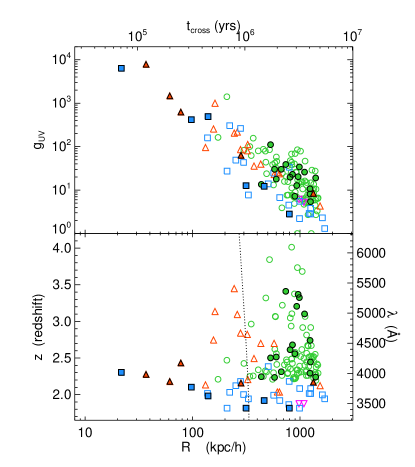
Figure 1.— Distribution of foreground quasar redshifts, transverse separations, and ionizing fluxes probed by the background quasar sightlines. The upper plot shows ionizing flux versus proper separations, which explains the general $R^{-2}$ trend. The lower plot shows foreground quasar redshift versus proper separations and the y-axis on the right indicates the wavelength of the Ly$\alpha~{}\lambda 1215.67$ Å transition at this redshift. The (blue) squares have a Keck (LRIS-B) spectrum of the background quasar, (red) triangles have Gemini (GMOS) background spectra, (magenta) upside down triangles have MMT (Blue Channel) background spectra, and (green) circles have SDSS background spectra. Filled symbols outlined in black have an optically thick absorber at the foreground quasar redshift (see Table 1) and open symbols have no absorber. The region to the left of the dotted line is excluded by the SDSS fiber collision limit of $\theta=55^{\prime\prime}$, which explains the paucity of SDSS background spectra there. The follow-up Keck/Gemini/MMT spectra probe angular separations an order of magnitude smaller than the fiber collision limit, allowing us to probe the foreground quasar environment down to $20~{}{\rm\ kpc}/h$ where the ionizing flux is $\sim 10,000$ times the UV background.

3.3. Voigt Profile Fitting

For all of the systems which were flagged by the initial visual inspection, we estimated the H I column density by fitting the Ly$\alpha$ profiles using standard practice. Namely, we over-plotted a Voigt profile on the Ly$\alpha$ transition, and centered the profile according to the redshift of metal-lines, if present. Otherwise, the redshift of the absorber was allowed to be a free parameter in the fit. The fits are done ‘by-eye’, which is to say we do not minimize a $\chi^{2}$ because the error in the fit is dominated by systematic uncertainty related to the quasar continuum placement and line-blending. Conservative error estimates are adopted to account for this uncertainty. In all cases, we assume a Doppler parameter $b$, which is typical of the high $z$ Ly$\alpha$ forest (e.g. Kirkman & Tytler 1997). In general, the fits are insensitive to the Doppler parameter parameter because most of the leverage in the fit comes from the damping wings of the line-profile; we assume $b=30\rm\ km\ s^{-1}$. See Prochaska et al. (2005) for more discussion on Voigt profile fits to Ly$\alpha$ absorption profiles.

The completeness and false positive rate of our survey are sources of concern. Line-blending, in particular, can significantly depress the continuum near the Ly$\alpha$ profile and mimic a damping wing, biasing the column density high. To investigate these issues we consider three objects in our sample for which we have both SDSS spectra and independent echelle observations. We obtained archived spectra of the background quasars SDSSJ 0303$-$0023, and SDSSJ 1204$+$0221, observed with the High Resolution Echelle Spectrometer (HIRES; Vogt et al. 1994) (FWHM $\approx 10~{}{\rm km~{}s}^{-1}$) on the Keck-I telescope, and SDSSJ 1429$-$0145, observed with the Magellan Inamori Kyocera Echelle spectrograph (MIKE; Bernstein et al. 2003) (FWHM $\approx 10~{}{\rm km~{}s}^{-1}$). For SDSSJ0303$-$0023, the column density of $\log N_{\rm HI}=18.95\pm 0.2$ measured form the SDSS spectrum is in good agreement $\log N_{\rm HI}=18.9\pm 0.2$ from the echelle spectrum. Likewise, for SDSSJ 1204$+$0221 we measured $\log N_{\rm HI}=19.7\pm 0.25$ from the SDSS data and $\log N_{\rm HI}=19.7\pm 0.2$ from HIRES. However, for SDSSJ1429$-$0145 we measure a total column of $\log N_{\rm HI}=19.55\pm 0.3$ from the SDSS data; whereas the echelle data gives $\log N_{\rm HI}=18.8\pm 0.2$, a value $2.5\sigma$ lower than the SDSS value. The source of the error is line blending, but we note that this absorber was located blueward of the quasars Ly$\beta$ emission line, in a ‘crowded’ part of the spectrum because of the presence of both the Ly$\alpha$ and Ly$\beta$ forests.

Based on visually inspecting 149 background quasar spectra and and the comparison with the echelle data for three systems, we suspect that our survey is $\sim 90\%$ complete for $\log N_{\rm HI}>19.3$ for all the Keck/Gemini/MMT spectra and the SDSS spectra with SNR${}_{\rm bg}>3$ (75%), or 123 of the 149 spectra we searched. For SDSS spectra with lower SNR${}_{\rm bg}>2$, our completeness limit is probably closer to $\log N_{\rm HI}>20$. A more careful examination of the completeness and false positive rate of Lyman limit systems identified in spectra of the resolution and SNR used here is definitely warranted. Statistical studies based on our sample which attempt to quantify the abundance of absorbers near foreground quasars (Hennawi & Prochaska 2006a), will suffer from a ‘Malmquist’ type bias because line-blending biases lower column densities upward, and the line density of absorbers $dN/dz$, is a steep function of column density limit. Finally, our completeness is likely to be higher and the false positive rate lower at $z\sim 2$, as compared higher redshifts ($z\sim 3$), because the mean flux decrement of the Ly$\alpha$ forest absorption decreases with decreasing redshift, and thus line blending causes less confusion.

3.4. Quasar-Absorber Sample

We present relevant quantities for the quasar-absorber pairs discovered in our survey in Table 1. All systems with $\log N_{\rm HI}>17.2$ are included; however those systems with column densities $\log N_{\rm HI}<18.3$ are included as LLSs based on the identification of definite Lyman limit absorption (i.e. $z_{\rm fg}>3.2$). In the next section (§ 4), we describe in detail how we estimated the foreground quasar redshifts and redshift errors which are listed in Table 1. The emission line which was used to compute this redshift is also noted in the Table.

The quantity $g_{\rm UV}=1+F_{\rm QSO}/F_{\rm UVB}$ in Table 1, is the maximum enhancement of the quasars ionizing photon flux over that of the extragalactic ionizing background, at the location of the background quasar sightline, assuming that the quasar emission is isotropic. It is the maximal enhancement because we assumed the distance is given by the transverse component alone. A discussion of how $g_{\rm UV}$ was computed is provided in Appendix A.

The distribution of foreground quasar redshifts, transverse separations, and ionizing fluxes probed by all of our projected pair sightlines is illustrated by the scatter plot in Figure 1. The filled symbols outlined in black indicate the sightlines which have an optically thick absorption line system (see Table 1) and open symbols are sightlines without an absorber. Note that the closest pairs are predominantly at redshift $z\sim 2$, because this is where quasar pair selection is most efficient (see Richards et al. 2002a; Hennawi et al. 2006a).

A list of tentative absorbers near quasars, for which we could not be sure that $\log N_{\rm HI}>17.2$, is published in Table 2 of Appendix B. Higher SNR and higher resolution spectra are required to make definitive conclusions about these systems; they are a valuable set of targets for future research. Coordinates and SDSS five band photometry of the quasar pairs in Tables 1 and 2 are provided in Tables 3 and 4, respectively, of Appendix C.

To summarize, we searched 149 projected quasar pair sightlines with transverse proper distances $22~{}h^{-1}{\rm\ kpc}<R<1.7~{}h^{-1}{\rm\ Mpc}$ away from foreground quasars in the redshift range $1.8<z<4.0$. Keck spectra accounted for 25 of the background quasar spectra, 19 came from Gemini, 2 from the MMT and the remaining 103 were from the SDSS. Of these sightlines, 25 had angular separations below the SDSS fiber collision limit ($\Delta\theta<55^{\prime\prime}$) with the Keck/Gemini/MMT accounting for all but three of these. We discovered 27 LLSs within $\Delta v=1500~{}{\rm km~{}s}^{-1}$ of the foreground quasar redshifts, of which 17 are super-LLSs with $\log N_{\rm HI}>19$.

4. Estimating Systemic Redshifts

The primary rest-frame ultraviolet quasar emission lines which are redshifted into the optical for $z\gtrsim 2$ quasars are: Ly$\alpha$ $\lambda 1216$, N V $\lambda 1240$, C IV $\lambda 1549$, C III] $\lambda 1908$, and Mg II $\lambda 2798$. The redshifts determined from these lines can differ by up to $\sim 3000~{}{\rm km~{}s}^{-1}$ from systemic, due to outflowing/inflowing material in the broad line regions of quasars (Gaskell 1982; Tytler & Fan 1992; Vanden Berk et al. 2001; Richards et al. 2002b). A redshift determined from the narrow ($\sigma\lesssim 200~{}{\rm km~{}s}^{-1}$) forbidden emission lines [O II] $\lambda 3727$ or [O III] $\lambda 5007$, are the best predictors of systemic redshift; but at $z\gtrsim 2$, measurements of these lines would require spectra covering the near infrared.

For example, redshifts are most uncertain when estimated from the C IV emission line: Richards et al. (2002b) found a median blueshift of 824$~{}{\rm km~{}s}^{-1}$ from Mg II with a dispersion about the median of 511$~{}{\rm km~{}s}^{-1}$, but with a tail extending to blueshifts as large as 3000 $~{}{\rm km~{}s}^{-1}$. Furthermore, Mg II has a median shift of 97$~{}{\rm km~{}s}^{-1}$ and a dispersion of 269$~{}{\rm km~{}s}^{-1}$ about [O III], which is used to define the systemic frame (Richards et al. 2002b). The implied average redshift uncertainty between C IV and [O III] (systemic) is thus $\gtrsim 600~{}{\rm km~{}s}^{-1}$. In addition, the C IV blueshift is luminosity dependent Gaskell82;Richards02, such that simply adding a median offset to a C IV line center can bias redshifts and result in larger errors. The quasar redshifts computed by the SDSS spectroscopic pipeline are the result of a maximum likelihood procedure which involves fitting of multiple emission lines simultaneously (see e.g. Stoughton et al. 2002), a procedure which will not result in robust systemic redshift estimates.

In light of these issues, we recompute the systemic redshifts of all the foreground quasars published in Table 1. Note that the spectra of foreground quasars used to compute these redshifts come from a variety of instruments (see Table 1) and they have varying SNRs and spectral coverage. Some are from the SDSS, for others we have high SNR Keck LRIS-R spectra covering $\lambda=5000-9500$ Å, and for others we have only Gemini GMOS spectra with $\sim 1500$ Å of coverage centered on the Ly$\alpha$ forest and typically extending to $\sim 1350$ Å in the quasar rest-frame.

For our spectra with full wavelength coverage (SDSS and LRIS-R), we begin by fitting the sum of a Gaussian plus a linear continuum (both in $\log\lambda$) to the primary emission lines C IV, C III], and Mg II if present, where the line-widths and centers are free parameters. We also include components for the weaker lines He II $\lambda 1640$ and Al III$\lambda 1857$, since they can be significantly blended with C IV and C III], respectively, thus contributing to the background and influencing the placement of the continuum. Guided by these fits, we calculate the mode of each line using the relation mode = 3 $\times$ median - 2$\times$ mean, applied to the upper $\approx$ 60% of the emission line. This is a more robust estimator than the centroid or median for slightly skewed profiles in noisy data. Specifically, we compute the mode of all spectral pixels within $\pm 1.5\sigma$, of the Gaussian line center which have flux

$$f_{\rm\lambda}>\frac{0.6A_{i}}{\sqrt{2\pi\sigma_{i}}}+C_{\rm\lambda}+\sum_{j\neq i}\frac{A_{j}}{\sqrt{2\pi\sigma_{j}}}e^{-\left(\log_{10}\lambda-\log_{10}\lambda_{j}\right)^{2}/2\sigma_{j}^{2}}$$ (2)

where $A_{i}$, $\log_{10}\lambda_{i}$, and $\sigma_{i}$, are the amplitude, central wavelength, and dispersion, of the best fit Gaussian to the $i$th emission line and $C_{\rm\lambda}$ is the linear continuum. The sum represents the effective background due to other nearby lines.

Given these line centers, a redshift is computed for each line. Redshifts are computed using the average velocity shift from systemic, defined with respect to the [O III] emission lines, where we use the shifts measured by Vanden Berk et al. (2001) and Richards et al. (2002b). A median SNR $>5$ over the line is required for it to be used as a redshift estimator. At high SNR, the intrinsic velocity shifts and line asymmetries will dominate over errors in line centering. In this case, our error estimates are motivated by the dispersion measurements of Richards et al. (2002b). For lower SNR, line centering errors can become significant, however we do not explicitly estimate this error contribution. Instead, we simply flag low SNR redshift determinations and dilate their errors by ‘hand’. Redshifts and errors are assigned to the 27 foreground quasars in Table 1 according to the following procedure:

• Use Mg II if it is present ($z\lesssim 2.2$). The redshift error is $\pm 300~{}{\rm km~{}s}^{-1}$ (6 systems).

• If Mg II is not present or has low SNR, C III] is used. The error is $\pm 500~{}{\rm km~{}s}^{-1}$ (13 systems)

• If neither Mg II nor C III] can be used, the redshift is computed from C IVThe error is $\pm 1000~{}{\rm km~{}s}^{-1}$ (3 systems).

• If neither Mg II, C III], or C IV have SNR $<$ 5, all are fit simultaneously for the redshift, using Gaussians plus continua (similar to SDSS pipeline procedure). The error is $\pm 1500~{}{\rm km~{}s}^{-1}$ (1 system).

• If C IV is unavailable because of limited spectral coverage (i.e. Gemini GMOS spectra), the redshift is computed from cross correlation with a composite quasar template (Vanden Berk et al. 2001). The redshift error is $\pm 1500~{}{\rm km~{}s}^{-1}$ (4 systems).

5. Notes on Individual Absorption Systems

The Keck, Gemini, and SDSS spectra of both the foreground and background quasars from Table 1 are shown in Figure 2. The right panels show show closeups of the H I absorption in the background quasar spectra and our best fit Ly$\alpha$ profiles. Below we describe how each system was fit and highlight interesting details.

SDSSJ 0036$+$0839 The SDSS spectrum of the background quasar reveals strong absorption features of C II $\lambda 1334$, Si IV $\lambda 1393,1403$, C IV $\lambda 1548,1550$, Si II $\lambda 1526$ and possibly O I $\lambda 1302$ and Si II $\lambda 1304$. A strong feature is coincident with Si II $\lambda 1260$, but this could be a Ly$\alpha$ forest absorption line. Centered on the redshift of the metal lines at $z=2.5647\pm 0.00005$, our Voigt profile fit to the H I Ly$\alpha$ gives $\log N_{\rm HI}=18.95\pm 0.35$. A redshift of $z_{\rm fg}=2.569$ is measured from the foreground quasars C III] emission line with an error of $\pm 500~{}{\rm km~{}s}^{-1}$. The velocity difference of $|\Delta v|=360~{}{\rm km~{}s}^{-1}$ from the absorber is within this error estimate.

SDSSJ 0127$+$1507 While most of the systems in Table 1 contain only two quasars, there are five quasars within $5^{\prime}$ of each other in the region surrounding SDSSJ 0127+1507 at redshifts $2.60$, $2.38$, $2.18$,$2.08$, and $1.81$ (denoted ABCDE). Along these sightlines, we identify two absorption systems in SDSSJ 0127+1507A ($z_{\rm bg}=2.60$; $\Delta\theta=131.0^{\prime\prime}$) and SDSSJ 0127+1507B ($z_{\rm bg}=2.38$; $\Delta\theta=51.9^{\prime\prime}$) with Ly$\alpha$ profiles indicating an optically thick absorber near the redshift of the foreground quasar SDSSJ 0127+1507E ($z_{\rm fg}=1.818$). No significant metal-line absorption is observed in either background quasar spectrum. Voigt profile fits to the two profiles give $z=1.819\pm 0.001$ and $\log N_{\rm HI}=18.6\pm 0.4$ toward SDSSJ0127+1508A and $z=1.1818\pm 0.001$ with $\log N_{\rm HI}=18.9\pm 0.3$ toward SDSSJ0127+1507B. We further identify additional strong Ly$\alpha$ absorption features in the spectrum of the background quasar J0127+1507C $(z_{\rm bg}=2.18;\Delta\theta=35^{\prime\prime})$, but we cannot precisely determine their $N_{\rm HI}$ values, and hence whether an optically thick absorber is present (see Table 2). The fourth background quasar SDSSJ 0127+1507D ($(z_{\rm bg}=2.18;\Delta\theta=163.1^{\prime\prime})$ shows no signs of significant Ly$\alpha$ absorption at the redshift $z_{\rm fg}=1.818$. Coordinates and photometry for all five members of this projected group of quasars are given in Table 5 of Appendix B.

SDSSJ 0225$-$0739 We detect strong Si II $\lambda 1526$ and Al II $\lambda 1670$ in the background quasar spectrum, which identify the redshift of the absorber at $z=2.4476\pm 0.0007$, coincident with the foreground quasar at $z_{\rm fg}=2.440$. Our fit to the Ly$\alpha$ profile is complicated by O VI emission from the quasar but yields the value $\log N_{\rm HI}=19.55\pm 0.2$ dex. The velocity difference of $|\Delta v|=690~{}{\rm km~{}s}^{-1}$ from the absorber is in excess of our estimated foreground quasar redshift error of $\pm 500~{}{\rm km~{}s}^{-1}$.

SDSSJ 0239$-$0106 The SDSS spectrum of the background quasar reveals strong absorption features of Si II $\lambda 1526$, Fe II $\lambda 1608$ and Al II $\lambda 1670$ at a redshift $z=2.3025\pm 0.0007$. Our estimate of the foreground quasar redshift is $z_{\rm fg}=2.308$ is particularly uncertain ($\pm 1500~{}{\rm km~{}s}^{-1}$) because of large BAL features. There is an apparently strong Ly$\alpha$ profile at this redshift in the SDSS spectrum but the SNR${}_{\rm fg}=1.8$ in this region is too low for a meaningful fit. As described in § 2, we acquired a low-dispersion LRIS-B spectrum of this pair to improve the fit, and it is these spectra which are shown in Figure 2. The metal-lines are detected in the LRIS-B spectrum of the background quasar, and a fit to the Ly$\alpha$ profile gives $\log N_{\rm HI}=20.45\pm 0.2$ dex. This absorber, therefore, satisfies the damped Ly$\alpha$ threshold ($\log N_{\rm HI}>20.3$). It was not included in the Prochaska et al. (2005) compilation, however, because of the low SNR of the SDSS spectrum in this region.

SDSSJ 0256$+$0039 The SDSS spectrum of the background quasar shows a weak C IV absorption system at $z=3.387\pm 0.001$ and a Lyman limit system with consistent redshift. There may also be weak absorption from Si II $\lambda 1260$ and Si IV $\lambda 1393,1402$. An examination of the Ly$\alpha$ profile at this redshift shows a significant feature, centered at $z_{Ly\alpha}=3.387$. A fit indicates an H I column density of $\log N_{\rm HI}=19.25\pm 0.25$ is allowed by the data, but this value is very uncertain because of the low SNR and lack of evidence for significant damping wings. The presence of an LLS sets a lower limit of to the H I column density $\log N_{\rm HI}>17.2$, unless the limit corresponds to another absorber nearby in redshift. The redshift of the foreground quasar $z_{\rm fg}=3.387$ is consistent with the redshift of the absorber.

SDSSJ 0303$-$0023 There is an absorption system showing very strong Si IV and C IV lines at $z=2.7243\pm 0.0007$ in the spectrum of the background quasar, which is $500~{}{\rm km~{}s}^{-1}$ away from the foreground quasar at $z=2.718$ ($\pm 1000~{}{\rm km~{}s}^{-1}$). Weak absorption consistent with Al II $\lambda 1670$ is observed at this redshift, but no significant detection of Fe II $\lambda 1608$ ($W_{\lambda}<100$mÅ). A strong Ly$\alpha$ profile is consistent with the C IV lines, although with nominal line centroid blueward of the metal-line absorption ($z_{Ly\alpha}=2.723$). If we constrain the fit by the C IV redshift, the red wing of Ly$\alpha$ provides the only constraint on the fit and we find $\log N_{\rm HI}=18.95\pm 0.20$. If we allow the redshift to be a free parameter, the best fit solution is $\approx 0.1$ dex larger. As mentioned in the previous section, we have independent echelle data for this background quasar and a fit to the Ly$\alpha$ profile gave $\log N_{\rm HI}=18.9\pm 0.20$, consistent with our measurement from the lower resolution SDSS spectrum.

SDSSJ0338-0005 This damped Ly$\alpha$ system shows a series of metal-line transitions including the Mg II doublet. The redshift of the gas is $z=2.2290\pm 0.0007$ and the foreground quasar is at $z=2.239$, but with large error, $\pm 1500~{}{\rm km~{}s}^{-1}$. The absorber is a member of the SDSS-DR3 DLA catalog and Prochaska et al. (2005) report an H I column density of $\log N_{\rm HI}=20.9\pm 0.15$ dex.

SDSSJ0800+3542 This absorber is notable for showing strong N V $\lambda 1238,1242$ absorption, which is rarely ever observed in LLSs. There is also significant absorption due to Si II $\lambda 1260$ and C II $\lambda 1334$, as well as the Fe II $\lambda 1608$ and Al II $\lambda 1670$ transitions. The metal line profiles are centered at $z=1.9828\pm 0.0007$ and are accompanied by a Ly$\alpha$ profile with $\log N_{\rm HI}=19.0\pm 0.15$, according to our fit. The absorber redshift is in good agreement with that of the foreground quasar, $z_{\rm fg}=1.983$.

SDSSJ0814+3250 Similar to SDSSJ0800+3524, this absorption system shows remarkably strong N V absorption in the spectrum of the background quasar, as well as several other metal transitions (Si II, C II, Si IV). The redshift of these metal-lines is $z=2.1792\pm 0.0007$. At the corresponding position of H I Ly$\alpha$ there is significant absorption, although oddly, the largest optical depth occurs 1.2Å away from the line centroid predicted by the metal lines. We have fit the Ly$\alpha$ profile with two H I components, one centered at $z=2.1792$ and an additional component at $z=2.1778$. Our best solution has $\log N_{\rm HI}=18.50\pm 0.2$ for each component. There is significant degeneracy between the two components, especially if one does not demand a component at $z=2.1792$. However, the total column density is well constrained and has a value of $\log N_{\rm HI}=18.80\pm 0.2$ dex. The foreground quasar is at $z_{\rm fg}=2.182\pm 1500~{}{\rm km~{}s}^{-1}$, which is $|\Delta v|=280~{}{\rm km~{}s}^{-1}$ away from the absorber (at $z=2.1792$), but well within the uncertainty of the foreground quasar redshift.

SDSSJ0833+0813 This system shows likely Si II $\lambda 1526$ and possible C IV absorption at $z=2.505\pm 0.001$ and a strong corresponding Ly$\alpha$ profile. If we adopt the metal line redshift, our best fit is a multi-component model with $\log N_{\rm HI}=19.45\pm 0.3$. But, there is a small chance that this profile is the blend of several $\log N_{\rm HI}\approx 18$ absorbers and that the total $\log N_{\rm HI}<19$. The metal line redshifts are $980~{}{\rm km~{}s}^{-1}$ from the foreground quasar at $z_{\rm fg}=2.516$, but this velocity difference is comparable to its redshift error $\pm 1000~{}{\rm km~{}s}^{-1}$.

SDSSJ0852+2637 The foreground quasar redshift ($z=3.203$) is sufficiently high that the SDSS spectrum covers the Lyman limit region. We do detect a break due to the Lyman limit at $912$ Å  and its corresponding Ly$\alpha$ profile at $z=3.211\pm 0.001$, in the background quasar spectrum. There are no detected metal-line transitions, which is not uncommon for Lyman limit systems at the resolution of the SDSS spectra. We estimate the column density to be $\log N_{\rm HI}=19.25\pm 0.4$. There is a $|\Delta v|=550~{}{\rm km~{}s}^{-1}$ between the absorber and the foreground quasar redshift ($z_{\rm fg}=3.203$), but this is within our estimated $\pm 1500~{}{\rm km~{}s}^{-1}$ margin of error on the latter.

SDSSJ0902+2841 Similar to SDSSJ0852+2637, the background quasar spectrum covers the Lyman limit at the redshift of the foreground quasar. The SDSS spectrum of the background quasar reveals a Lyman limit system at $z=3.342\pm 0.005$, corresponding to an offset by $|\Delta v|=1200~{}{\rm km~{}s}^{-1}$ from the foreground quasar redshift $z_{\rm fg}=3.325$. This offset is more than twice the estimated redshift error ($\pm 500~{}{\rm km~{}s}^{-1}$) from the C III] emission line of the foreground quasar. No significant metal-line absorption is identified. There is a Ly$\alpha$ absorption profile with centroid consistent with the Lyman limit redshift. There appears to be residual flux in the line profile, but the data has insufficient SNR in this region to say definitively. While a column density $\log N_{\rm HI}>19$ is permitted by the data, we suspect the actual value is less than this. Thus we set a conservative lower limit of $\log N_{\rm HI}>17.2$ based on the presence of a limit.

SDSSJ1134+3409 This quasar exhibits a very strong C IV system at $z=2.2879\pm 0.005$ and possible detections of Si II $\lambda 1526$ and Al II $\lambda 1670$ in the background quasar spectrum. There is a corresponding Ly$\alpha$ profile with rest equivalent width $W_{\lambda}=4.9\pm 0.2$Å. Our fit to this profile gives $\log N_{\rm HI}=19.5\pm 0.3$ if we tie the redshift to the C IV absorption. We derive a $+0.3$ dex larger value if we allow the redshift to vary as a free parameter to $z=2.2865$. Either redshift is in good agreement ($|\Delta v|<400~{}{\rm km~{}s}^{-1}|$) with the foreground quasar at $z_{\rm fg}=2.291$.

SDSSJ1152+4517 The background quasar spectrum has a strong Ly$\alpha$ absorption feature at $z=2.3158\pm 0.0010$ and a C IV absorption system at $z=2.31323\pm 0.0007$, significantly offset from the Ly$\alpha$ feature. Our profile fit to Ly$\alpha$ gives $\log N_{\rm HI}=19.1\pm 0.3$ assuming the redshift $z=2.3158$. The absorber is offset by $|\Delta v|=370~{}{\rm km~{}s}^{-1}$ from the foreground quasar at $z_{\rm fg}=2.312\pm 500~{}{\rm km~{}s}^{-1}$, but this is within the redshift error.

SDSSJ1204+0221 For this quasar, we have both GMOS and SDSS spectra. Figure 2 shows the GMOS spectra (left) of both pairs, but we used the SDSS data to fit the Ly$\alpha$ profile (right), because this spectrum gave coverage of more of the metal lines. A series of strong metal transitions were identified at $z=2.4402\pm 0.0003$ and our fit to the Ly$\alpha$ profile gives $\log N_{\rm HI}=19.7\pm 0.25$. A fit to the column density using an echelle spectrum (HIRES) of this object gives the same value. The absorber redshift is offset by $|\Delta v|=370~{}{\rm km~{}s}^{-1}$ from that of the foreground quasar $z_{\rm fg}=2.436\pm 1500~{}{\rm km~{}s}^{-1}$, but the error on this determination is large.

SDSSJ1213+1207 A strong Ly$\alpha$ absorption feature is identified at $z=3.4110\pm 0.0007$ in the background quasar spectrum, which is in good agreement with the foreground quasar redshift $z_{\rm fg}=3.411$. A likely coincident C IV absorption feature is also identified. The SDSS data provide coverage of the Lyman limit at this redshift, and the break is detected, although the SNR of the data in this region is poor. Our Voigt profile fit to the Ly$\alpha$ feature gives $\log N_{\rm HI}=19.25\pm 0.3$.

SDSSJ1306+6158 The LRIS-B spectrum of the background quasar shows a damped Ly$\alpha$ system at $z=2.1084\pm 0.0007$, consistent ($|\Delta v|=200~{}{\rm km~{}s}^{-1}$) with the redshift of the foreground quasar, $z_{\rm fg}=2.111\pm 300~{}{\rm km~{}s}^{-1}$. A series of metal-line transitions outside the Ly$\alpha$ forest are identified, which constrain the redshift well. Our single component fit to the Ly$\alpha$ profile gives $\log N_{\rm HI}=20.30\pm 0.15$.

SDSSJ1312+0002 The low SNR spectrum of the background quasar shows the following metal-line transitions at $z=2.6688\pm 0.0007$: O I $\lambda 1302$, Si II $\lambda 1304$, C II $\lambda 1334$, Si IV $\lambda 1393,1402$, Si II $\lambda 1526$, C IV $\lambda 1548,1550$, Al II $\lambda 1670$, and likely Fe II $\lambda 2382$. A strong Ly$\alpha$ absorption profile is consistent with this redshift. Although the SNR is low ($\approx 2$ per pixel), the H I column density is consistent with the DLA threshold $\log N_{\rm HI}=20.3\pm 0.3$. This profile was fit with a similar value by Prochaska et al. (2005) but not included in their sample because of the low SNR. The absorber redshift is offset by $|\Delta v|=200~{}{\rm km~{}s}^{-1}$ from that of the foreground quasar $z_{\rm fg}=2.671$, but within its error ($\pm 500~{}{\rm km~{}s}^{-1}$).

SDSSJ1426+5002 We identify an absorption system in this SDSS background quasar spectrum with very strong metal-lines including detections of the weak Si II $\lambda 1808$ and Zn II $\lambda 2026$ transitions at $z=2.2247\pm 0.0007$. Prochaska et al. (2005) reported an $N_{\rm HI}$ column density for this absorber below the DLA threshold ($\log N_{\rm HI}>20.3$) and we similarly find $\log N_{\rm HI}=20.00\pm 0.15$ here. This low column density is rather remarkable relative to the the strong metal-line absorption. The redshift of the absorber is offset by $|\Delta v|=1330~{}{\rm km~{}s}^{-1}$ from the foreground quasar redshift $z_{\rm fg}=2.239$, which is more than twice our estimated redshift error of $\pm 500$ from the C III] emission line of the foreground quasar.

SDSSJ1427-0121 Our high SNR GMOS spectrum of the background quasar reveals several metal-line absorption features redward of Ly$\alpha$. Near the redshift of the foreground quasar, we identify Si II $\lambda 1260$, C II $\lambda 1334$, and Si IV absorption. These lines show multiple components spanning over $1000~{}{\rm km~{}s}^{-1}$. We identify similar structure in the Ly$\alpha$ profile, although, the bluest component of the metal lines does not correspond to significant H I absorption, similar to the case for SDSSJ 0814$+$3250. We have fit the Ly$\alpha$ complex with 3 components at $z=2.2762,2.2788$, and $2.2828$ with $\log N_{\rm HI}=14,18.85$, and $18.80$, respectively. The low column density $\log N_{\rm HI}=14$ component results from the lack of significant optical depth in the bluest component. Because the features are well separated, there is minimal degeneracy in the fit, although the uncertainty is still $\approx 0.25$ dex for each component. The two features at $z=2.2788$ and $z=2.2828$ differ in redshift by $366~{}{\rm km~{}s}^{-1}$, greater than the $300~{}{\rm km~{}s}^{-1}$ maximum value suggested by O’Meara et al. (2006) in combining multiple component absorption systems to one. Thus, we take the component at $z=2.2788$ with $\log N_{\rm HI}=18.85$ as the quasar companion, since it is closest to the foreground quasar systemic redshift $z_{\rm fg}=2.278$, differing by only $|\Delta v|=50~{}{\rm km~{}s}^{-1}$.

SDSSJ1429-0145 The SDSS spectrum of the background quasar shows an absorption system with large EW metal-line features of Si II $\lambda 1526$, C IV $\lambda 1548,1550$, Fe II $\lambda 1608$ and Al II $\lambda 1670$ at a redshift $z=2.6235\pm 0.0007$, in relatively good agreement with the foreground quasar redshift at $z_{\rm fg}=2.628$. We identify a strong Ly$\alpha$ profile with rest equivalent width $W_{\lambda}=3.8$Å; however, the centroid of this profile lies blueward of the peak in the optical depth of the metal-line transitions. There is also evidence for weak absorption in the metal-line profiles redward of the dominant absorption. Fitting the profile with two components, we derive $\log N_{\rm HI}=19.3\pm 0.3$ at $z=2.6235$ and $\log N_{\rm HI}=19.2\pm 0.3$ at $z=2.6267$. Similar to the absorbers associated with SDSSJ0814+3250, the two values for the two components are degenerate, but their total H I column density, $N_{\rm HI}=19.55\pm 0.3$ is well constrained. As mentioned in § 3, we have also examined echelle spectra of this background quasar, and a significantly lower column density was measured, $\log N_{\rm HI}=18.8\pm 0.2$, with the difference being caused by unresolved line-blending in the SDSS spectrum. It is this lower value which is listed in Table 1.

SDSSJ1430-0120 The background quasar exhibits a pair of damped Ly$\alpha$ systems from the Prochaska et al. (2005) compilation at $z=3.0238$ and $z=3.115$ with $\log N_{\rm HI}=21.10\pm 0.2$ and $\log N_{\rm HI}=20.50\pm 0.2$, respectively. The DLA at $z=3.115$ is $|\Delta v|=960~{}{\rm km~{}s}^{-1}$ away from the foreground quasar $z_{\rm fg}=3.102$; however the foreground quasar redshift has a large associated error $\pm 1500~{}{\rm km~{}s}^{-1}$. Also, there is no apparent metal-line absorption for the DLA coincident with the quasar, and the redshift is not tightly constrained by the Ly$\alpha$ profile fit: we estimate an uncertainty of $\delta z=\pm 0.002$ ($\pm 150~{}{\rm km~{}s}^{-1}$).

SDSSJ1545+5112 We identify a strong Ly$\alpha$ profile at $z=2.243\pm 0.001$ in the background quasar spectrum of this pair, in good agreement with the foreground quasar redshift $z_{\rm fg}=2.240$. Weak absorption features consistent with O I $\lambda 1302$, C II $\lambda 1334$ and possibly C IV are present; but we note the absence of any obvious Si II $\lambda 1260$, calling these identifications into question, because the oscillator strengths of these transitions are comparable. A Voigt profile fit to the Ly$\alpha$ gives $\log N_{\rm HI}=19.45\pm 0.3$.

SDSSJ1621+3508 Our LRIS-R spectrum of this bright background quasar exhibits a Mg II system at $z=1.9309\pm 0.0007$, in good agreement with the foreground quasar redshift $z_{\rm fg}=1.931$. It also shows metal absorption from C II, C IV, and Si II. A corresponding strong H I Ly$\alpha$ absorption profile is identified in our LRIS-B spectra and the best fit column density is $\log N_{\rm HI}=18.7\pm 0.2$.

SDSSJ1635+3013 The SDSS spectrum of this background quasar shows metal-line absorption from Si II $\lambda 1526$ and Al II $\lambda 1670$ at a $z=2.5025\pm 0.001$. The foreground quasar at $z_{\rm fg}=2.493\pm 500~{}{\rm km~{}s}^{-1}$ is offset from the absorber by $|\Delta v|=820~{}{\rm km~{}s}^{-1}$ which is significant compared to the foreground quasar redshift error. The Ly$\alpha$ profile at the redshift of the metals lines appears significantly blended with other coincident Ly$\alpha$ absorption transitions. The H I value is thus poorly constrained. We obtain a fit of $\log N_{\rm HI}=19.35\pm 0.3$ but report a conservative lower limit of $\log N_{\rm HI}>19$.

SDSSJ2347+1501 This triple system consists of a background quasar at SDSSJ2347$+$1501A at $z_{\rm bg}=2.29$, and two foreground quasars: SDSSJ2347$+$1501B ($z_{\rm fg}=2.157$; $\Delta\theta=47.3$) and SDSSJ2347$+$1501C ($z_{\rm fg}=2.171$; $\Delta\theta=223.0$). We identify S IV absorption at $z=2.176\pm 0.001$, near the redshifts of the foreground quasars. There is a corresponding strong Ly$\alpha$ absorption feature, but it appears to be a blend of two components. Our best fit profile, which is not very well constrained, gives $\log N_{\rm HI}=18.55$ at $z=2.174$ and $\log N_{\rm HI}=18.1$ at $z=2.177$. These values are highly correlated but the absence of significant damping wings limits the total H I column density to be $\log N_{\rm HI}<19$, and we place a lower limit on the total column density of $\log N_{\rm HI}<18.3$. The absorber is offset by $|\Delta v|=1770~{}{\rm km~{}s}^{-1}$ from SDSSJ2347$+$1501B at $z_{\rm fg}=2.157\pm 1000~{}{\rm km~{}s}^{-1}$, and $|\Delta v|=380~{}{\rm km~{}s}^{-1}$ from SDSSJ2347$+$1501C at $z_{\rm fg}=2.171\pm 500~{}{\rm km~{}s}^{-1}$. The large offset from SDSSJ2347$+$1501B exceeds the limit of our search ($\pm 1500~{}{\rm km~{}s}^{-1}$). If part of this offset is due to Hubble flow, the quasar would be separated from the absorber by $\gtrsim>5h^{-1}{\rm\ Mpc}$ in the radial direction, much larger than the $R=282~{}h^{-1}{\rm\ kpc}$ transverse separation.

6. Cosmological Applications of Optically Thick Absorbers Near Quasars

The cosmological applications of optically thick absorption line systems near quasars are many. They include measurement of the clustering of absorbers around quasars, determining the spatial distribution of neutral gas in LLSs and DLAs, fluorescent Ly$\alpha$ emission from LLSs, constraints on the emission geometry and lifetimes of quasars, and studying the enrichment and velocity fields in the environs of luminous quasars. We discuss each of these in turn.

6.1. Clustering of Absorbers around Quasars

A conspicuous feature of Figure 1 is the high covering factor of absorbers for small separations. Six out of eight projected sightlines with $R<150~{}h^{-1}{\rm\ kpc}$ have a LLS coincident with the foreground quasar, of which four are super-LLSs ($\log N_{\rm HI}>19$). We previously estimated that the probability of a random quasar-super-LLS coincidence is $\sim 2\%$ (see beginning of § 3); thus the average number expected in eight sightlines is $\sim 0.16$. This factor of $\sim 25$ increase in the number of small scale quasar-absorber coincidences provides significant evidence that these absorbers are strongly clustered around quasars. It is particularly interesting that in the projected pairs which show absorption, an LLS is seen in the transverse direction only – none of the foreground quasars show an intrinsic or proximate optically thick absorber along the line of sight.

Although they are rare, proximate absorbers with $z_{\rm abs}\sim z_{\rm em}$ are occasionally observed in single lines of sight. In a recent study, Russell et al. (2005), found that the abundance of DLAs is enhanced by a factor of $\sim 2$ near quasars, which they attributed to the clustering of the DLA counterpart galaxies around quasars. The high covering factor for $R<150~{}h^{-1}{\rm\ kpc}$ in Figure 1 suggests a significantly larger enhancement in the transverse direction. We measure the transverse quasar-absorber correlation function and compare it to the abundance of proximate absorbers in the second paper of this series (Hennawi & Prochaska 2006a).

An asymmetry between the strength of clustering in the radial and transverse direction could be the hallmark of anisotropy or obscuration of quasar emission. If the emission were highly anisotropic, optically thick absorbers along the line-of-sight might be evaporated by the ionizing flux; whereas, transverse absorbers could lie in shadowed regions, and hence survive. This speculation gains some credibility in light of the recent null detections of the transverse proximity effect in the Ly$\alpha$ forests of projected quasar pairs (Crotts 1989; Dobrzycki & Bechtold 1991; Fernandez-Soto, Barcons, Carballo, & Webb 1995; Liske & Williger 2001; Schirber, Miralda-Escudé, & McDonald 2004; Croft 2004, but see Jakobsen et al.2003). Although these studies are each based only on a handful of projected pairs, they all come to similar conclusions: the amount of (optically thin) Ly$\alpha$ forest absorption, in the background quasar sightline near the redshift of the foreground quasar, is larger than average rather than smaller – the opposite of what is expected from the transverse proximity effect. Our Keck, Gemini, MMT, and SDSS spectra will be used to study the transverse proximity effect in an upcoming paper (Hennawi et al. 2006b).

Finally, if obscuration of the quasars emission is indeed the explanation for the anisotropic clustering pattern suggested by Figure 1, we would naively expect the transverse covering factor to be approximately equal to the average fraction of the solid angle obscured. Studies of Type II quasars and the X-ray background suggest that quasars with luminosities comparable to our foreground quasar sample ($M_{\rm B}<-23$) have $\sim 30\%$ of the solid angle obscured (Ueda et al. 2003; Barger et al. 2005; Treister & Urry 2005), although these estimates are highly uncertain. This seems to be at odds with the high covering factor (6/8) for having an absorber with $\log N_{\rm HI}>17.2$) that we observe on the smallest scales ($R<150~{}h^{-1}{\rm\ kpc}$), although our statistics are clearly very poor.

6.2. Fluorescent Ly$\alpha$ Emission: Shedding Light On Lyman Limit Systems

Are there LLSs or DLAs that can self-shield the intense ionizing flux of a nearby quasar? How do we know if these systems are being illuminated? – By observing the fluorescent glow of their recombination radiation. Optically thick H I clouds in ionization equilibrium with a photoionizing background, re-emit $\sim 60\%$ of the ionizing radiation they absorb as fluorescent Ly$\alpha$ recombination line photons (Gould & Weinberg 1996; Zheng & Miralda-Escudé 2002; Cantalupo et al. 2005; Adelberger et al. 2005; Kollmeier et al. 2006). All attempts to detect this fluorescent radiation from LLSs illuminated by the ambient UV background have been unsuccessful (Bunker et al. 1998; Marleau et al. 1999; Becker 2005), despite $\gtrsim 60$ hour integrations on 10m telescopes (Becker 2005). However, if a nearby quasar illuminates an absorber, as could be the case for the quasar-absorber pairs in Table 1 the fluorescent surface brightness is enhanced by a factor of $g_{\rm UV}$, making it much easier to detect. Indeed, Adelberger et al. (2005) reported a possible detection of fluorescence from a quasar-DLA pair at $z=2.84$, which was serendipitously discovered in their LBG survey(Steidel et al. 1999; Adelberger et al. 2003). The ionizing flux is enhanced by a factor of $g_{\rm UV}\simeq 4850$, owing to their extremely luminous foreground quasar $r\simeq 16$ (but also see Francis & Bland-Hawthorn 2004, who failed to detect fluorescence around a bright $B=17.6$ quasar).

In Table 1 we publish seven new quasar-absorber pairs with enhancements $g_{\rm UV}>100$, with largest being $\sim 7900$ for SDSSJ1427$-$0121. This corresponds to fluorescent surface brightnesses of $\mu_{{\rm Ly}\alpha}=19.5-24.3~{}{\rm mag~{}arcsec}^{-2}$, if the foreground quasars emit isotropically. This potential 5-10 magnitude increase in the expected surface brightness would constitute a breakthrough for the study of fluorescence from optically thick absorbers. It is intriguing that two of the three systems which have enhancements of $g_{\rm UV}>1000$ (SDSSJ0814$+$3250 and SDSSJ1427$-$0121) for which we have high SNR ratio moderate resolution spectra, both have H I Ly$\alpha$ absorption misaligned with the regions of highest metal line optical depth. These peculiar absorption profiles are suggestive of emission in the LLS trough (see Figure 2 and § 5). This suggestion is particularly intriguing when one considers that proximate DLAs observed along the line of sight to single quasars, seem to preferentially exhibit Ly$\alpha$ emission superimposed on the Ly$\alpha$ absorption trough (Moller et al. 1998; Ellison et al. 2002). We present a detailed discussion of fluorescent emission from our quasar-LLS pairs in the third paper of this series (Hennawi & Prochaska 2006b).

Finally, because the fluorescent emission from a LLS comes from the a thin ionized ‘skin’ where $\tau_{\rm LL}\sim 1$ (Gould & Weinberg 1996), the size of this region can be measured if fluorescent emission is detected. Indeed, Adelberger et al. (2005) constrained the emitting region from their fluorescing DLA to be $\gtrsim 1.5^{\prime\prime}$, or a proper size of $r_{\rm DLA}=8.5~{}h^{-1}{\rm\ kpc}$. A statistical study of fluorescent emission from LLSs illuminated by quasars, can measure the distribution of sizes for optically thick absorbers, as well as the relationship between size and observed H I column. The fluorescent flux also measures the ionizing flux at the self-shielding boundary, which, when combined with the size, constrains the density and distribution of gas in LLSs and DLAs, providing physical insights into the morphologies of high redshift galaxies which are difficult to derive from the resonance line observations of absorption line spectroscopy.

6.3. Constraining Quasar Lifetimes

In addition to serving as a valuable laboratory for studying fluorescent emission and the size and nature of LLSs, the detection of fluorescence from an LLS illuminated by a quasar can place interesting constraints on the lifetimes of individual quasars. A LLS near a quasar acts like a mirror, ‘reflecting’ $\sim 60\%$ of the ionizing photons absorbed from the quasar towards us. However, this reflection can only be detected provided that ionizing flux of the quasar has not changed significantly for a time longer than the light crossing time to the LLS. The light crossing time corresponding to $60^{\prime\prime}$ ($1.2~{}h^{-1}{\rm\ Mpc}$) from a $z=2.5$ quasar is $1.1\times 10^{6}$ yr.

Currently, the lower limit on the intermittency of quasar emission comes from observations of the proximity effect (Bajtlik et al. 1988; Scott et al. 2000), in the Ly$\alpha$ forests near quasars. The presence of a proximity effect implies that the IGM has had time to reach ionization equilibrium with the quasars increased ionizing flux, giving the lower limit $t_{\rm burst}\gtrsim 10^{4}$ yr (Martini 2004). However, owing to the large amplitude of intrinsic Ly$\alpha$ forest fluctuations, many quasars must be averaged over to detect the proximity effect, hence the intermittency of individual quasars cannot be constrained with this technique (Scott et al. 2000). A positive detection of fluorescence allows one to place much stronger constraints on quasar intermittency and lifetimes, with the added advantage that the lifetimes of individual quasars can be constrained.

6.4. Probing the AGN Environment with High-Resolution Spectroscopy

If the background quasar is sufficiently bright ($R\lesssim 19$), then one can obtain a high-resolution spectrum on a 10m class telescope. These data provide more accurate measurements of $N_{\rm HI}$ for absorbers with $\log N_{\rm HI}<20$. More importantly, these data yield accurate ionic column density measurements critical to the analysis of physical conditions (e.g. ionization state, gas density, metallicity). It is noteworthy that several of the absorbers exhibit the N V doublet in the low-dispersion data. This ion is rarely observed in quasar absorption line systems and suggests an environment with a significantly enhanced UV radiation field. The spectra also reveal the velocity field of gas in the vicinity of bright AGN where feedback processes (e.g. jets, merger activity) may be important. In the case of SDSS1204 we measure a velocity width $\Delta v\approx 600~{}{\rm km~{}s}^{-1}$ for the Si⁺, C⁺, and C⁺³ ions. We will present and analyze these observations in Paper IV of the series (Prochaska & Hennawi 2006).

7. Summary

We searched 149 moderate resolution background quasar spectra, from Gemini, Keck, MMT, and the SDSS for optically thick absorbers in the vicinity of $1.8<z<4.0$ foreground quasars. We presented 27 new quasar-LLS pairs with column densities $17.2<\log N_{\rm HI}<20.9$ and transverse distances of $22~{}h^{-1}{\rm\ kpc}<R<1.7~{}h^{-1}{\rm\ Mpc}$ from the quasars, corresponding to factors of $g_{\rm UV}=5-8000$ larger ionizing fluxes than the ambient UV background, if the quasars emit isotropically. The observed probability of intercepting an absorber is very high for small separations: six out of eight projected sightlines with transverse separations $R<150~{}h^{-1}{\rm\ kpc}$ have an absorber coincident with the foreground quasar, of which four have $N_{\rm HI}>10^{19}{\rm cm}^{-2}$. The covering factor of $N_{\rm HI}>10^{19}{\rm cm}^{-2}$ absorbers is thus $\sim 50\%$ (4/8) on these small scales, whereas $\lesssim 2\%$ would have been expected at random.

Techniques for estimating quasar systemic redshifts from noisy rest frame UV spectra were presented and used to compute the systemic redshifts of the foreground quasars in our sample. An important area for future work is to obtain near-IR ($H$-band) spectra of the $z\gtrsim 2$ foreground quasars to determine more accurate redshifts from the narrow ($\sigma\lesssim 200~{}{\rm km~{}s}^{-1}$) forbidden emission lines [O II] $\lambda 3727$ or [O III] $\lambda 5007$, which are the best predictors of systemic redshift.

Much larger samples of optically thick absorbers near quasars are easily within reach, and can be compiled in a modest amount of observing on a 6-10m class telescopes. Richards et al. (2004) constructed a photometric catalog of $z<3$ quasars from the SDSS imaging data which has high completeness and efficiency, and photometric redshifts accurate to $|\Delta z|\lesssim 0.3$. Indeed, many of the projected quasar pairs shown in Figure 1 were selected from this catalog (see Hennawi et al. 2006a). The number density of $z_{\rm phot}>1.8$ quasars in the photometric catalog is $10.5$ deg², so that the total number of projected sightlines expected with $\Delta\theta<25^{\prime\prime}$ ($R\lesssim 150~{}h^{-1}{\rm\ kpc}$) for the current $\sim 8000~{}{\rm deg}^{2}$ of SDSS imaging is 140, of which $\sim 70$ would have super-LLSs if we extrapolate from the $\sim 50\%$ covering factor of such systems observed in this study. At moderate resolution, sufficient SNR can be obtained in a 30 minute exposure at Keck, and about 2.5 times longer at the MMT. Thus, a 7 night program on a 10m class telescope, or 18 nights at 6m class, targeting the closest projected pairs would result in a factor of about 20 more quasar-absorber pairs, with $R<150~{}h^{-1}{\rm\ kpc}$ and $\log N_{\rm HI}\gtrsim 19$, than the four published here. If a multi-slit setup were used, wider separation projected pairs come for ‘free’, since these quasars can be targeted and observed simultaneously on the same masks, as was done for our Keck observations. Finally, we note that a similar survey of projected quasar pairs using the techniques presented here can be used to search for Mg II, C IV or other absorption lines sytem near foreground quasars (Bowen et al. 2006b; Prochter, Hennawi, & Prochaska 2006).

A sample of $\sim 100$ LLSs near quasars would be of tremendous cosmological interest, providing new opportunities to characterize the environments, emission geometry, and radiative histories of quasars, as well as new laboratories for studying fluorescent emission from optically thick absorbers and the physical nature of LLSs and DLAs.

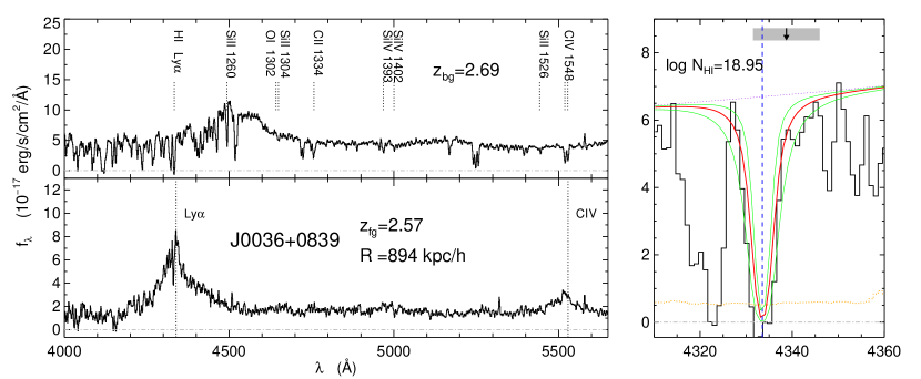
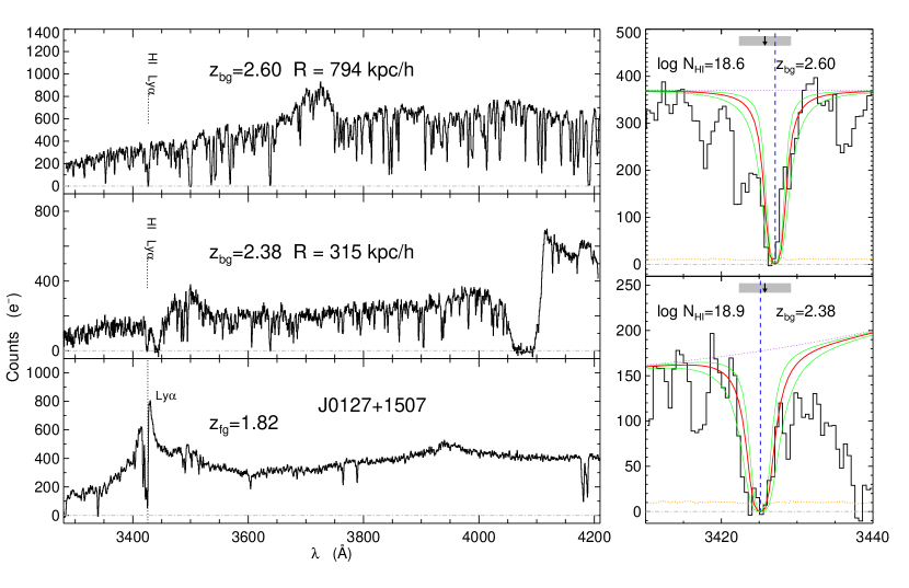
Figure 2.— Spectra of projected quasar pairs with optically thick absorbers coincident with the foreground quasar redshift. The left panels show the background (upper) and foreground (lower) quasars. Some of the metal line transitions discussed in § 5 and indicated by labels and dotted lines on the background quasar spectrum. Quasar emission lines are indicated on the foreground quasar spectrum. The panels on the right show a closeup of the H I Ly$\alpha$ absorption in the background quasar spectrum. The (red) central curves indicate the best Voigt profile fit, (green) upper and lower curves show the fits corresponding to our $\pm 1\sigma$ column density errors, and (blue) dashed lines indicate the redshifts of absorption components. The upper (purple) dotted line indicates the continuum level used for the fit and the lower (orange) dotted line indicates the noise level. The arrow indicates the foreground quasar redshift and the (gray) rectangle indicates our estimate of the redshift error. Three quasars are shown on the left for the triple systems SDSSJ0127$+$1507 and SDSSJ2347$+$1501. Cross hatched regions in the spectra of SDSSJ1204$+$0221 and SDSSJ2347$+$1501 indicate gaps in the spectral coverage of the Gemini GMOS spectrograph.

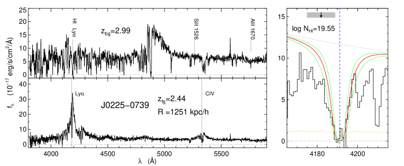
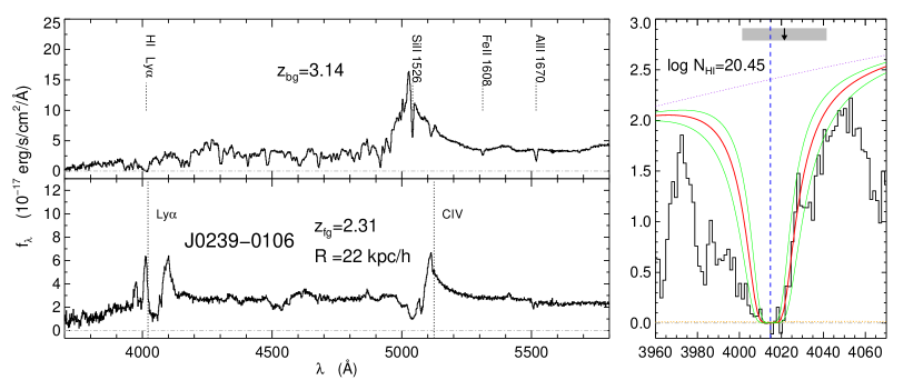
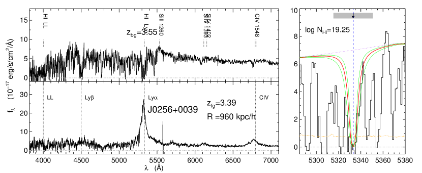
Figure 2.— continued.

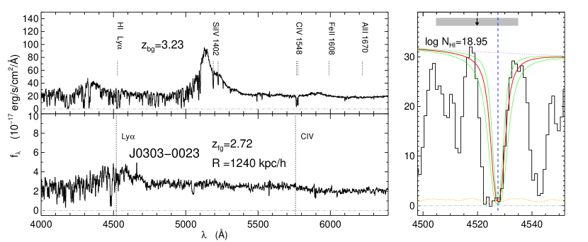
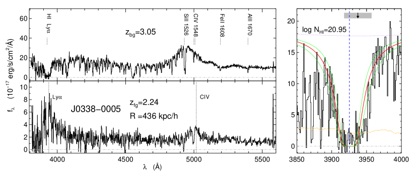
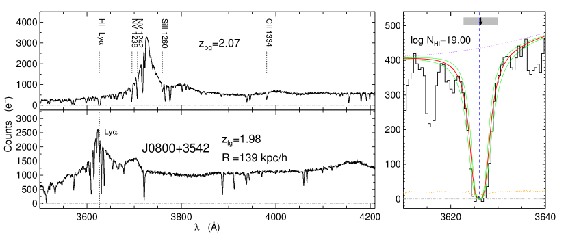
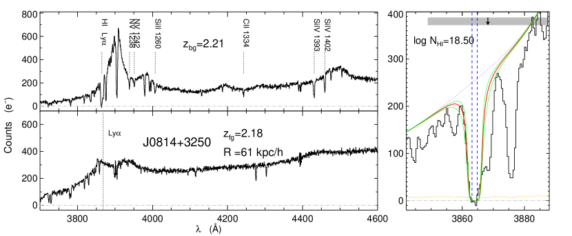
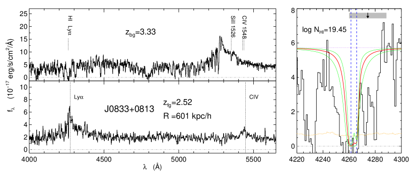
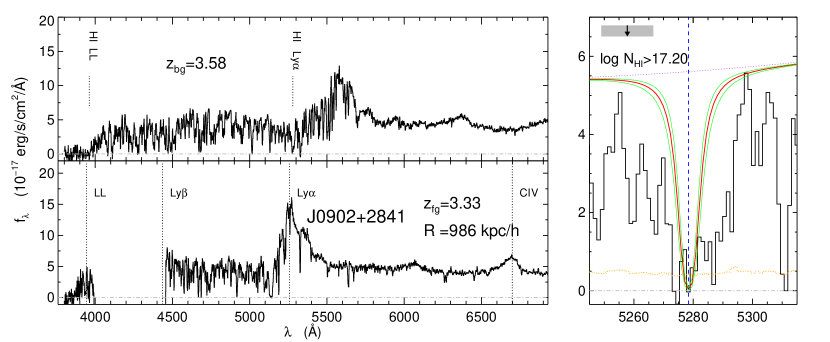
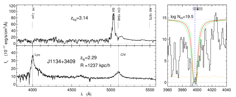
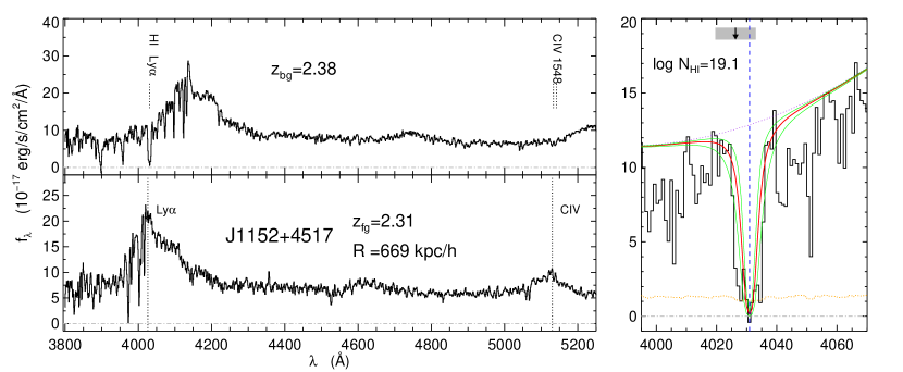
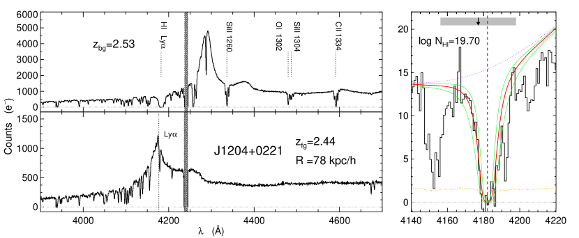
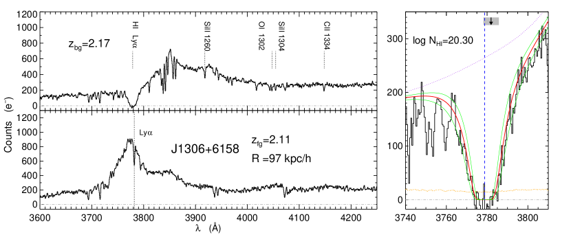
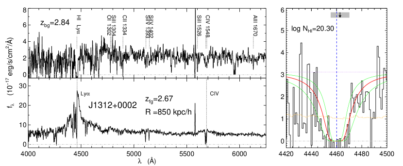
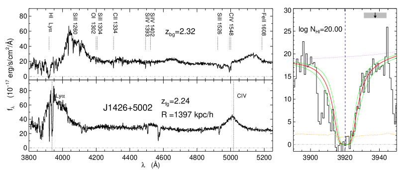
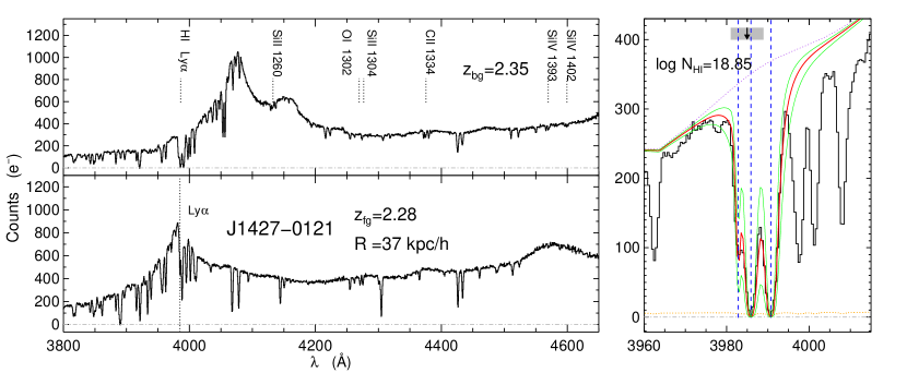
Figure 2.— continued.

Figure 2.— continued.

Figure 2.— continued.

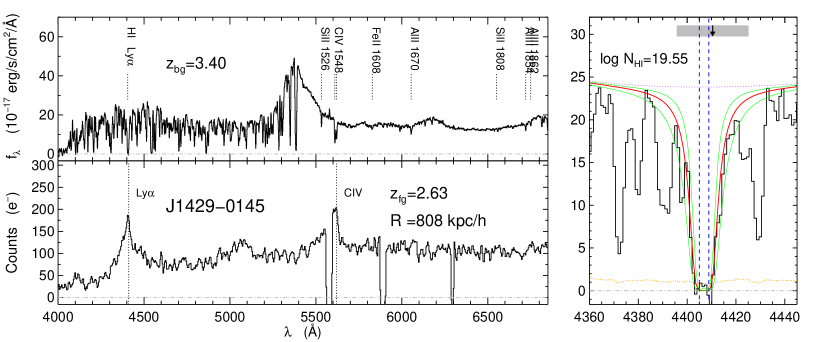
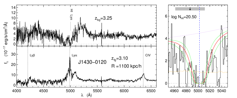
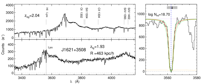
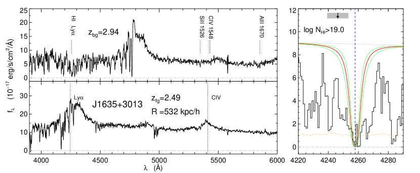
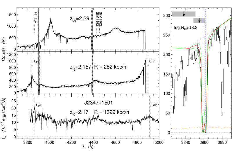
Figure 2.— continued.

Figure 2.— continued.

Figure 2.— continued.

Figure 2.— continued.

Figure 2.— continued.

Appendix A UV Enhancement

In this appendix we describe how we computed the quantity

$$g_{\rm UV}\equiv 1+\frac{F_{\rm QSO}}{F_{\rm UVB}},$$ (A1)

which is the maximum enhancement of the quasars’ ionizing photon flux over that of the extragalactic ionizing background, at the location of the background quasar sightline, assuming that the quasar emits isotropically.

The ionizing photon number flux $F_{\rm UVB}$ (photons s^-1 cm^-2) due to the UV background is

$$F_{\rm UVB}=\pi\int_{\nu_{\rm LL}}^{\infty}\frac{J_{\nu}}{h\nu}d\nu,$$ (A2)

where $\nu_{\rm LL}=13.6~{}{\rm eV}/h$ is the Lyman limit frequency, $h$ is Planck’s constant, and $J_{\nu}$ is the mean specific intensity of the UV background (erg s^-1 cm^-2 ster^-1 Hz^-1). For the intensity of the UV background, we use the version computed by F. Haardt & P. Madau (2006, in preparation), which considers the emission from observed quasars and galaxies after it is filtered through the IGM to yield the UVB as a function of redshift.

The ionizing photon number flux from a quasar of specific luminosity $L_{\rm\nu}$ (erg s^-1 cm^-2 Hz^-1) at a proper distance $r_{\rm Q}$ is

$$F_{\rm QSO}=\frac{1}{4\pi r^{2}_{\rm Q}}\int_{\nu_{\rm LL}}^{\infty}\frac{L_{\nu}}{h\nu}d\nu.$$ (A3)

We assume that the quasars’ spectral energy distribution obeys the power law form $L_{\nu}=L_{\nu_{\rm LL}}(\nu/\nu_{\rm LL})^{-\alpha_{\rm Q}}$, blueward of $\nu_{\rm LL}$. Telfer et al. (2002) measured an average power law slope of $\alpha_{\rm Q}=1.57$ blueward of wavelengths $\lesssim 1200$ Å, with the transition to this slope occurring in the range $\lambda=1200-1300$ Å.

The luminosity density at the Lyman limit for a quasar at redshift $z$ is,

$$L_{\nu_{\rm LL}}=\frac{4\pi d_{L}^{2}(z)}{\left(1+z\right)}f_{\nu_{0}},$$ (A4)

where $d_{\rm L}$ is the luminosity distance and $f_{\nu_{0}}$ is the specific flux of the quasar as observed on Earth at the redshifted frequency $\nu_{0}=\nu_{\rm LL}/(1+z)$. We define the apparent magnitude at the Lyman limit, measured by an observer on Earth at the redshifted frequency $\nu_{0}$ according to

$$f_{\nu_{0}}=10^{-0.4\left(48.60+m_{912}\right)}~{}{\rm erg}~{}{\rm s}^{-1}~{}{\rm cm}^{-2}~{}{\rm Hz}^{-1}.$$ (A5)

For the majority of the quasars in Table 1 the Lyman limit is below the atmospheric cutoff. Furthermore, even for higher redshifts, determining $m_{912}$ from our spectroscopic observations or the SDSS broad band magnitudes is complicated by the absorption from the Lyman-$\alpha$ forest and LLSs. Our goal is then to compute $m_{\rm 912}$ given the SDSS apparent magnitude of a quasar, measured in the rest frame near-UV. To this end, we tie the Telfer et al. (2002) power law spectrum to the composite quasar spectrum of Vanden Berk et al. (2001) at the wavelength $1285$Å, which is a clean region free of emission lines and in the wavelength range ($\lambda=1200-1300$ Å) where (Telfer et al. 2002) observed the transition to a spectral index of $\alpha_{\rm Q}$. We then compute the ‘k-correction’ between $m_{\rm 912}$ and the bluest SDSS filter, which is also redward of the Ly$\alpha$ line in the observed frame, by convolving the Vanden Berk et al. (2001) template with the SDSS filter curve. We work with a filter redward of Ly$\alpha$ to avoid the Ly$\alpha$ forest of the quasar, which is not correctly included in the quasar template.

Appendix B Tentative Optically Thick Absorbers Near Quasars

Relevant quantities for a sample of tentative quasar-absorber pairs, for which we could not be sure that $\log N_{\rm HI}>17.2$ are given in Table 2. Higher SNR and higher resolution spectra are required to make definitive conclusions about these systems, making them an interesting set of targets for future research. Coordinates and SDSS five band photometry of these objects are given in Table 4 of Appendix C.

Table 2Tenative Optically Thick Absorbers Near Quasars

Name	zbg	zfg	$\Delta\theta$	$R$	zabs	$\left|\Delta v\right|$	$\Delta v_{\rm fg}$	$g_{\rm UV}$	Redshift	Fg	Bg
			(′′)	($h^{-1}{\rm\ kpc}$)		($~{}{\rm km~{}s}^{-1}$)	($~{}{\rm km~{}s}^{-1}$)			Inst.	Inst.
SDSSJ0127$+$1507	2.38	2.173	46.9	280	2.177	0370	300	261	Mg II	SDSS	LRIS-B
SDSSJ0225$+$0048	2.82	2.692	100.3	574	2.710	1430	500	023	C III]	SDSS	GMOS
SDSSJ0340$+$0018	3.34	2.661	207.8	1192	2.6788	1420	500	007	C III]	SDSS	SDSS
SDSSJ1132$+$5338	3.34	2.919	188.9	1060	2.914	0350	500	010	C III]	SDSS	SDSS
SDSSJ1314$+$6213	3.14	2.335	69.3	409	2.328	670	500	079	C III]	SDSS	SDSS
SDSSJ1356$+$6133	2.17	2.013	22.9	138	2.026	1290	1500	159	C III]	SDSS	LRIS-B
SDSSJ1719$+$2919	3.29	3.072	106.4	588	3.069	0220	1000	030	C IV	SDSS	SDSS

Appendix C Coordinates and Photometry

Coordinates and SDSS five band photometry of the quasars in Tables 1 and 2 are listed below. We also list coordinates and photometry for all five members of the projected group of quasars associated with SDSSJ 0127$+$1507 in Table 5.

Table 3Coordinates and Photometry for Projected Quasar Pairs in Table 1

Name	RA (2000)	Dec (2000)	z	$u$	$g$	$r$	$i$	$z$
SDSSJ0036$+$0839A	00:36:43.45	$+$08:39:44.4	2.69	20.13	19.54	19.28	19.30	19.00
SDSSJ0036$+$0839B	00:36:53.85	$+$08:39:36.2	2.57	20.90	20.37	20.34	20.30	20.33
SDSSJ0127$+$1508A	01:27:44.85	$+$15:08:58.0	2.60	20.95	20.56	20.50	20.38	20.33
SDSSJ0127$+$1507B	01:27:42.57	$+$15:07:38.4	2.38	21.21	20.61	20.55	20.71	20.70
SDSSJ0127$+$1506E	01:27:43.53	$+$15:06:48.4	1.82	21.21	21.25	21.14	20.94	20.99
SDSSJ0225$-$0739A	02:25:59.78	$-$07:39:38.9	3.04	21.92	19.53	19.17	19.07	19.06
SDSSJ0225$-$0743B	02:25:56.50	$-$07:43:07.3	2.44	20.70	19.95	19.82	19.58	19.30
SDSSJ0239$-$0106A	02:39:46.44	$-$01:06:44.1	3.12	22.20	20.28	19.99	20.00	19.93
SDSSJ0239$-$0106B	02:39:46.43	$-$01:06:40.4	2.31	21.26	20.61	20.56	20.54	20.19
SDSSJ0256$+$0039A	02:56:47.15	$+$00:39:01.2	3.55	18.22	17.08	16.65	30.89	16.47
SDSSJ0256$+$0036B	02:56:50.89	$+$00:36:11.3	3.39	22.23	20.23	19.96	19.87	20.08
SDSSJ0303$-$0023A	03:03:41.01	$-$00:23:21.9	3.22	19.48	17.48	17.27	17.25	17.26
SDSSJ0303$-$0020B	03:03:35.42	$-$00:20:01.1	2.72	20.38	19.89	19.67	19.46	19.26
SDSSJ0338$-$0005A	03:38:54.78	$-$00:05:21.0	3.05	19.65	18.42	18.21	18.18	18.14
SDSSJ0338$-$0006B	03:38:51.83	$-$00:06:19.6	2.24	21.67	20.99	20.74	20.53	20.18
SDSSJ0800$+$3542A	08:00:48.74	$+$35:42:31.3	2.07	19.55	19.54	19.55	19.42	19.27
SDSSJ0800$+$3542B	08:00:49.90	$+$35:42:49.6	1.98	19.25	19.14	19.13	18.94	18.75
SDSSJ0814$+$3250A	08:14:19.59	$+$32:50:18.7	2.21	20.79	20.33	20.33	20.17	19.70
SDSSJ0814$+$3250B	08:14:20.38	$+$32:50:16.1	2.18	20.28	19.93	19.80	19.73	19.46
SDSSJ0833$+$0813A	08:33:28.07	$+$08:13:17.5	3.34	21.64	19.63	19.17	19.19	19.11
SDSSJ0833$+$0812B	08:33:21.61	$+$08:12:38.6	2.52	20.82	20.20	20.04	20.11	19.78
SDSSJ0852$+$2637A	08:52:37.93	$+$26:37:58.5	3.32	22.94	19.64	19.18	19.07	19.12
SDSSJ0852$+$2635B	08:52:32.16	$+$26:35:26.2	3.20	24.74	20.70	20.34	20.19	20.18
SDSSJ0902$+$2841A	09:02:34.54	$+$28:41:18.6	3.58	25.96	20.09	19.14	19.00	18.77
SDSSJ0902$+$2839B	09:02:23.33	$+$28:39:30.2	3.33	22.93	19.71	19.26	19.19	19.16
SDSSJ1134$+$3409A	11:34:44.22	$+$34:09:33.8	3.14	20.58	18.58	18.37	18.43	18.42
SDSSJ1134$+$3406B	11:34:53.94	$+$34:06:42.8	2.29	19.21	18.82	18.82	18.81	18.62
SDSSJ1152$+$4517A	11:52:00.54	$+$45:17:41.5	2.38	19.75	19.12	19.13	19.08	18.87
SDSSJ1152$+$4518B	11:52:10.43	$+$45:18:25.9	2.31	19.46	18.99	18.98	18.98	18.76
SDSSJ1204$+$0221A	12:04:16.69	$+$02:21:11.0	2.53	19.68	19.06	19.02	18.96	18.67
SDSSJ1204$+$0221B	12:04:17.47	$+$02:21:04.7	2.44	20.99	20.52	20.46	20.49	20.05
SDSSJ1213$+$1207A	12:13:10.72	$+$12:07:15.1	3.48	22.85	20.15	19.58	19.50	19.53
SDSSJ1213$+$1208B	12:13:03.26	$+$12:08:39.0	3.41	25.74	20.55	19.86	19.76	19.69
SDSSJ1306$+$6158A	13:06:03.55	$+$61:58:35.2	2.17	20.88	20.31	20.33	20.39	20.10
SDSSJ1306$+$6158B	13:06:05.19	$+$61:58:23.7	2.11	20.33	20.23	20.17	20.19	20.01
SDSSJ1312$+$0002A	13:12:13.30	$+$00:02:31.3	2.88	22.32	20.71	20.03	19.45	19.02
SDSSJ1312$+$0000B	13:12:13.84	$+$00:00:03.0	2.67	20.42	19.36	19.17	18.84	18.55
SDSSJ1426$+$5002A	14:26:28.02	$+$50:02:48.3	2.32	18.87	18.27	18.16	18.06	17.85
SDSSJ1426$+$5004B	14:26:05.79	$+$50:04:26.6	2.24	18.40	17.88	17.81	17.73	17.52
SDSSJ1427$-$0121A	14:27:58.73	$-$01:21:36.2	2.35	20.07	19.32	19.27	19.27	18.99
2QZJ1427$-$0121B	14:27:58.89	$-$01:21:30.4	2.28	19.83	19.26	19.15	19.13	19.08
SDSSJ1429$-$0145A	14:29:03.04	$-$01:45:19.4	3.39	21.51	18.58	17.96	17.78	17.64
2QZJ1429$-$0146B	14:29:10.81	$-$01:46:37.3	2.63	20.08	19.45	19.41	19.43	19.27
SDSSJ1430$-$0120A	14:30:06.42	$-$01:20:20.0	3.26	22.95	20.47	20.05	19.94	19.82
SDSSJ1429$-$0117B	14:29:57.09	$-$01:17:57.1	3.10	21.97	19.52	19.02	18.84	18.62
SDSSJ1545$+$5112A	15:45:34.60	$+$51:12:29.3	2.45	20.07	19.43	19.38	19.35	19.15
SDSSJ1545$+$5113B	15:45:44.15	$+$51:13:07.5	2.24	19.65	19.18	19.19	19.17	18.91
SDSSJ1621$+$3508A	16:21:45.42	$+$35:08:07.2	2.03	18.76	18.71	18.65	18.55	18.42
SDSSJ1621$+$3507B	16:21:41.02	$+$35:07:12.8	1.93	20.73	20.57	20.54	20.45	20.23
SDSSJ1635$+$3013A	16:35:00.06	$+$30:13:21.7	2.94	20.60	19.05	18.85	18.82	18.93
SDSSJ1634$+$3014B	16:34:56.16	$+$30:14:37.8	2.49	19.08	18.52	18.26	18.26	18.13
SDSSJ2347$+$1501A	23:47:03.24	$+$15:01:01.5	2.29	20.22	19.52	19.44	19.34	19.06
SDSSJ2347$+$1501B	23:47:04.25	$+$15:01:46.4	2.16	20.05	20.04	20.02	19.80	19.44
SDSSJ2346$+$1457C	23:46:57.26	$+$14:57:35.9	2.18	19.50	18.99	18.74	18.62	18.48

Note. — Coordinates, redshifts, and extinction corrected SDSS five band PSF photometry are given in the columns $u$, $g$, $r$, $i$, and $z$ for the projected quasar pairs in Table 1. The background and foreground quasars are labeled ‘A’ and ‘B’, respectively.

Table 4Coordinates and Photometry for Projected Quasar Pairs in Table 2

Name	RA (2000)	Dec (2000)	z	$u$	$g$	$r$	$i$	$z$
SDSSJ0127$+$1507A	01:27:42.57	$+$15:07:38.4	2.38	21.21	20.61	20.55	20.71	20.70
SDSSJ0127$+$1506B	01:27:41.20	$+$15:06:55.9	2.17	18.73	18.51	18.36	18.36	18.17
SDSSJ0340$+$0018A	03:40:14.25	$+$00:18:47.9	3.34	22.02	20.28	19.92	19.85	19.78
SDSSJ0340$+$0019B	03:40:00.92	$+$00:19:44.7	2.66	20.80	20.11	19.94	19.92	19.65
SDSSJ1132$+$5338A	11:32:06.14	$+$53:38:08.7	3.34	24.66	20.42	20.08	19.91	19.74
SDSSJ1131$+$5335B	11:31:50.70	$+$53:35:59.0	2.92	21.17	20.02	19.92	19.80	19.57
SDSSJ1314$+$6213A	13:14:29.24	$+$62:13:00.1	3.13	22.01	19.94	19.65	19.50	19.51
SDSSJ1314$+$6212B	13:14:19.52	$+$62:12:46.6	2.34	19.90	19.21	19.00	19.00	18.70
SDSSJ1356$+$6133A	13:56:29.54	$+$61:33:10.4	2.17	20.43	20.18	20.13	19.78	19.59
SDSSJ1356$+$6133B	13:56:32.44	$+$61:33:00.7	2.01	20.67	20.43	20.32	20.24	20.16
SDSSJ1719$+$2919A	17:19:32.94	$+$29:19:29.7	3.29	23.00	20.16	19.86	19.71	19.77
SDSSJ1719$+$2918B	17:19:37.87	$+$29:18:05.0	3.07	22.72	20.56	20.20	20.19	20.30

Note. — Coordinates, redshifts, and extinction corrected SDSS five band PSF photometry are given in the columns $u$, $g$, $r$, $i$, and $z$ for the projected quasar pairs in Table 2. The background and foreground quasars are labeled ‘A’ and ‘B’, respectively.

Table 5Coordinates and Photometry for the Five Quasars In the Projected Group SDSSJ0127$+$1507

Name	RA (2000)	Dec (2000)	z	$u$	$g$	$r$	$i$	$z$
SDSSJ0127$+$1508A	01:27:44.85	$+$15:08:58.0	2.60	20.95	20.56	20.50	20.38	20.33
SDSSJ0127$+$1507B	01:27:42.57	$+$15:07:38.4	2.38	21.21	20.61	20.55	20.71	20.70
SDSSJ0127$+$1506C	01:27:41.20	$+$15:06:55.9	2.18	18.73	18.51	18.36	18.36	18.17
SDSSJ0127$+$1504D	01:27:40.77	$+$15:04:10.3	2.08	19.93	20.07	20.03	19.86	19.57
SDSSJ0127$+$1506E	01:27:43.53	$+$15:06:48.4	1.82	21.21	21.25	21.14	20.94	20.99

Note. — Coordinates, redshifts, and extinction corrected SDSS five band PSF photometry are given in the columns $u$, $g$, $r$, $i$, and $z$ for the projected quasar pairs in Table 1. The background and foreground quasars are labeled ‘A’ and ‘B’, respectively.

References

- Abazajian et al. (2003) Abazajian, K., et al. 2003, AJ, 126, 2081
- Abazajian et al. (2004) Abazajian, K., et al. 2004, AJ, 128, 502
- Abazajian et al. (2005) Abazajian, K., et al. 2005, AJ, 129, 1755
- Adelberger et al. (2003) Adelberger, K. L., Steidel, C. C., Shapley, A. E., & Pettini, M. 2003, ApJ, 584, 45
- Adelberger & Steidel (2005) Adelberger, K. L., & Steidel, C. C. 2005, ApJ, 630, 50
- Adelberger et al. (2005) Adelberger, K. L., Steidel, C. C., Kollmeier, J. A., & Reddy, N. A. 2005, ArXiv Astrophysics e-prints, arXiv:astro-ph/0509229
- Alcock & Paczyński (1979) Alcock, C. & Paczyński, B. 1979, Nature, 281, 358
- Bahcall & Chokshi (1991) Bahcall, N. A. & Chokshi, A. 1991, ApJ, 380, L9
- Bahcall, Schmidt, & Gunn (1969) Bahcall, J. N., Schmidt, M., & Gunn, J. E. 1969, ApJ, 157, L77
- Bajtlik et al. (1988) Bajtlik, S., Duncan, R. C., & Ostriker, J. P. 1988, ApJ, 327, 570
- Barger et al. (2005) Barger, A. J., Cowie, L. L., Mushotzky, R. F., Yang, Y., Wang, W.-H., Steffen, A. T., & Capak, P. 2005, AJ, 129, 578
- Becker (2005) Becker, G. D., Presentation at IAU Colloquium 199, “Probing Galaxies Through Quasar Absorption Lines”, March 14-18, 2005 , Shanhai, China
- Bernstein et al. (2003) Bernstein, R., Shectman, S. A., Gunnels, S. M., Mochnacki, S., & Athey, A. E. 2003, Proc. SPIE, 4841, 1694
- Bouché & Lowenthal (2004) Bouché, N., & Lowenthal, J. D. 2004, ApJ, 609, 513
- Bowen et al. (2006b) Bowen, D. V., et al. 2006, submitted
- Brown, Boyle, & Webster (2001) Brown, M. J. I., Boyle, B. J., & Webster, R. L. 2001, AJ, 122, 26
- Bunker et al. (1998) Bunker, A. J., Marleau, F. R., & Graham, J. R. 1998, AJ, 116, 2086
- Cantalupo et al. (2005) Cantalupo, S., Porciani, C., Lilly, S. J., & Miniati, F. 2005, ApJ, 628, 61
- Castander et al. (2001) Castander, F. J., et al. 2001, AJ, 121, 2331
- Coil et al. (2006) Coil, A. L., et al. 2006, submitted
- Cooke et al. (2006) Cooke, J., Wolfe, A. M., Gawiser, E., & Prochaska, J. X. 2006, ApJ, 636, L9
- Croft (2004) Croft, R. A. C. 2004, ApJ, 610, 642
- Croom et al. (2004) Croom, S. M., Smith, R. J., Boyle, B. J., Shanks, T., Miller, L., Outram, P. J., & Loaring, N. S. 2004, MNRAS, 349, 1397
- Crotts (1989) Crotts, A. P. S. 1989, ApJ, 336, 550
- Dobrzycki & Bechtold (1991) Dobrzycki, A. & Bechtold, J. 1991, ApJ, 377, L69
- D’Odorico et al. (2002) D’Odorico, V., Petitjean, P., & Cristiani, S. 2002, A&A, 390, 13
- Ellison et al. (2002) Ellison, S. L., Yan, L., Hook, I. M., Pettini, M., Wall, J. V., & Shaver, P. 2002, A&A, 383, 91
- Faber et al. (2003) Faber, S. M., et al. 2003, Proc. SPIE, 4841, 1657
- Fernandez-Soto, Barcons, Carballo, & Webb (1995) Fernandez-Soto, A., Barcons, X., Carballo, R., & Webb, J. K. 1995, MNRAS, 277, 235
- Francis & Bland-Hawthorn (2004) Francis, P. J., & Bland-Hawthorn, J. 2004, MNRAS, 353, 301
- Fukugita et al. (1996) Fukugita, M., Ichikawa, T., Gunn, J. E., Doi, M., Shimasaku, K., & Schneider, D. P. 1996, AJ, 111, 1748
- Gaskell (1982) Gaskell, C. M. 1982, ApJ, 263, 79
- Gawiser et al. (2001) Gawiser, E., Wolfe, A. M., Prochaska, J. X., Lanzetta, K. M., Yahata, N., & Quirrenbach, A. 2001, ApJ, 562, 628
- Gould & Weinberg (1996) Gould, A., & Weinberg, D. H. 1996, ApJ, 468, 462
- Gunn et al. (1998) Gunn, J. E., et al. 1998, AJ, 116, 3040
- Gunn et al. (2006) Gunn, J. E., Siegmund, W. A., & Mannery, E. J. 2006, ArXiv Astrophysics e-prints, arXiv:astro-ph/0602326
- Haardt & Madau (1996) Haardt, F.,& Madau, P. 1996,ApJ, 461, 20
- Hennawi et al. (2006a) Hennawi, J. F., et al. 2006, AJ, 131, 1
- Hennawi et al. (2006b) Hennawi, J. F., et al. 2006, in preparation
- Hennawi & Prochaska (2006a) Hennawi, J. F. & Prochaska, J. X. 2006, in preparation
- Hennawi & Prochaska (2006b) Hennawi, J. F. & Prochaska, J. X. 2006, in preparation
- Hogg et al. (2001) Hogg, D. W., Finkbeiner, D. P., Schlegel, D. J., & Gunn, J. E. 2001, AJ, 122, 2129
- Hook et al. (2004) Hook, I. M., Jørgensen, I., Allington-Smith, J. R., Davies, R. L., Metcalfe, N., Murowinski, R. G., & Crampton, D. 2004, PASP, 116, 425
- Hui, Stebbins, & Burles (1999) Hui, L., Stebbins, A., & Burles, S. 1999, ApJ, 511, L5
- Jakobsen et al. (2003) Jakobsen, P., Jansen, R. A., Wagner, S., & Reimers, D. 2003, A&A, 397, 891
- Kirkman & Tytler (1997) Kirkman, D., & Tytler, D. 1997, ApJ, 484, 672
- Kollmeier et al. (2006) Kollmeier, J. A., et al., in preparation
- Liske & Williger (2001) Liske, J., & Williger, G. M. 2001, MNRAS, 328, 653
- Lupton et al. (2001) Lupton, R. H., Gunn, J. E., Ivezić, Z., Knapp, G. R., Kent, S., & Yasuda, N. 2001, ASP Conf. Ser. 238: Astronomical Data Analysis Software and Systems X, 10, 269
- Martini (2004) Martini, P. 2004, Coevolution of Black Holes and Galaxies, 169
- Marleau et al. (1999) Marleau, F. R., Bunker, A. J., & Graham, J. R. 1999, ASP Conf. Ser. 193: The Hy-Redshift Universe: Galaxy Formation and Evolution at High Redshift, 193, 262
- McDonald & Miralda-Escudé (1999) McDonald, P. & Miralda-Escudé, J. 1999, ApJ, 518, 24
- Meiksin (2005) Meiksin, A. 2005, MNRAS, 356, 596
- Moller et al. (1998) Moller, P., Warren, S. J., & Fynbo, J. U. 1998, A&A, 330, 19
- Møller et al. (2002) Møller, P., Warren, S. J., Fall, S. M., Fynbo, J. U., & Jakobsen, P. 2002, ApJ, 574, 51
- Oke et al. (1995) Oke, J. B., et al. 1995, PASP, 107, 375
- O’Meara et al. (2006) O’Meara, J. M., et al. 2006, in preparation
- Péroux et al. (2005) Péroux, C., Dessauges-Zavadsky, M., D’Odorico, S., Sun Kim, T., & McMahon, R. G. 2005, MNRAS, 363, 479
- Pier et al. (2003) Pier, J. R., Munn, J. A., Hindsley, R. B., Hennessy, G. S., Kent, S. M., Lupton, R. H., & Ivezić, Ž. 2003, AJ, 125, 1559
- Prochaska (1999) Prochaska, J. X. 1999, ApJ, 511, L71
- Prochaska et al. (2003) Prochaska, J. X., Gawiser, E., Wolfe, A. M., Cooke, J., & Gelino, D. 2003, ApJS, 147, 227
- Prochaska et al. (2005) Prochaska, J. X., Herbert-Fort, S., & Wolfe, A. M. 2005, ApJ, 635, 123
- Prochaska & Hennawi (2006) Prochaska, J. X., & Hennawi, J. F. 2006, in preparation
- Prochter, Hennawi, & Prochaska (2006) Prochter, G. E., Hennawi,J. F., & Prochaska, J. X. 2006, in preparation
- Richards et al. (2002a) Richards, G. T., et al. 2002, AJ, 123, 2945
- Richards et al. (2002b) Richards, G. T., Vanden Berk, D. E., Reichard, T. A., Hall, P. B., Schneider, D. P., SubbaRao, M., Thakar, A. R., & York, D. G. 2002, AJ, 124, 1
- Richards et al. (2004) Richards, G. T., et al. 2004, ApJS, 155, 257
- Russell et al. (2005) Russell, D. M., Ellison, S. L., & Benn, C. R. 2005, ArXiv Astrophysics e-prints, arXiv:astro-ph/0512210
- Schirber, Miralda-Escudé, & McDonald (2004) Schirber, M., Miralda-Escudé, J., & McDonald, P. 2004, ApJ, 610, 105
- Schneider et al. (2005) Schneider, D. P., et al. 2005, AJ, 130, 367
- Scott et al. (2000) Scott, J., Bechtold, J., Dobrzycki, A., & Kulkarni, V. P. 2000, ApJS, 130, 67
- Serber et al. (2006) Serber, W., et al.2005, about to be submitted.
- Smith et al. (2002) Smith, J. A., et al. 2002, AJ, 123, 2121
- Smith, Boyle, & Maddox (2000) Smith, R. J., Boyle, B. J., & Maddox, S. J. 2000, MNRAS, 313, 252
- Spergel et al. (2003) Spergel, D. N., et al. 2003, ApJS, 148, 175
- Steidel et al. (1999) Steidel, C. C., Adelberger, K. L., Giavalisco, M., Dickinson, M., & Pettini, M. 1999, ApJ, 519, 1
- Stoughton et al. (2002) Stoughton, C., et al. 2002, AJ, 123, 485
- Telfer et al. (2002) Telfer, R. C., Zheng, W., Kriss, G. A., & Davidsen, A. F. 2002, ApJ, 565, 773
- Treister & Urry (2005) Treister, E., & Urry, C. M. 2005, ApJ, 630, 115
- Tytler & Fan (1992) Tytler, D., & Fan, X.-M. 1992, ApJS, 79, 1
- Ueda et al. (2003) Ueda, Y., Akiyama, M., Ohta, K., & Miyaji, T. 2003, ApJ, 598, 886
- Vanden Berk et al. (2001) Vanden Berk, D. E., et al. 2001, AJ, 122, 549
- Vogt et al. (1994) Vogt, S. S., et al. 1994, Proc. SPIE, 2198, 362
- Yee & Green (1984) Yee, H. K. C. & Green, R. F. 1984, ApJ, 280, 79
- Yee & Green (1987) Yee, H. K. C. & Green, R. F. 1987, ApJ, 319, 28
- York et al. (2000) York, D. G., et al. 2000, AJ, 120, 1579
- Zheng & Miralda-Escudé (2002) Zheng, Z., & Miralda-Escudé, J. 2002, ApJ, 578, 33