Newtonian and Pseudo-Newtonian Hill Problem

Abstract

A pseudo-Newtonian Hill problem based on the Paczyński-Wiita pseudo-Newtonian potential that reproduces general relativistic effects is presented and compared with the usual Newtonian Hill problem. Poincaré maps, Lyapunov exponents and fractal escape techniques are employed to study bounded and unbounded orbits. In particular we consider the systems composed by Sun, Earth and Moon and composed by the Milky Way, the M2 cluster and a star. We find that some pseudo-Newtonian systems - including the M2 system - are more stable than their Newtonian equivalent.

1 Introduction

In the 19th century G.W. Hill [1] presented an approximation of the Moon-Earth-Sun system, where the movement of the Moon around the Earth was just perturbed by a distant Sun. This approximation became known as the Hill Problem. Nowadays, this approximation is still applied in solar system models where bodies in nearly circular orbits are perturbed by other far away massive bodies. Also, the Hill problem is very useful in the study of the stellar dynamics, e.g., consider a star in a star cluster this last orbiting around a galaxy. The star, the cluster, and the galaxy can be considered as the Moon, the Earth, and the Sun, respectively. Despite the fact that the potentials of the cluster and the galaxy are far from being the potentials of a point masses and their orbits are far from being circular the Hill problem can be taken as a first approximation and can easily accommodate necessary modifications, see for instance, Heggie [2].

The Hill Problem was first formulated in the realm of Newtonian dynamics. However, there exists extreme cases, like very massive bodies, black holes, and systems at great velocities, etc. wherein the Newtonian mechanics is no longer valid and relativistic corrections or a fully general relativistic approach is needed. The Hill problem was proved to be non-integrable by Meletlidou et al. [3], and is chaotic, as shown by Simó and Stuchi [4].

The aim of this paper is first to study a pseudo-Newtonian Hill problem obtained replacing the Newtonian potential by the Paczyński-Wiita [5] potential that reproduces in a rather simple way some aspects of the general relativistic dynamics. This is can be considered as a “zeroth order” approach to a general relativistic Hill problem. A more rigorous approach should consider a schema of systematic approximations within the realm of Einstein theory of gravitation like the schema of post-Newtonian approximations. Due to the mathematical complexity of the post-Newtonian approximations in this case it is worth to begin with the simpler, but not rigorous, treatment of the Hill problem based on the pseudo-Newtonian potential above mentioned. The results obtained will be used as a starting point for a more complete treatment of the same problem in a future work.

We shall compare the stability of orbits of the third body in the pseudo-Newtonian general relativistic simulation with the equivalent classical Newtonian system. In particular we shall study the Sun-Earth-Moon system and the three body problem associated with the Milky Way, the M2 cluster and a star.

In the Section 2 we review the Newtonian Hill problem, with its only integral of motion, the Jacobi integral. In Section 3 we present the pseudo-Newtonian Hill problem obtained obtained replacing the Newtonian potential by the Paczyński-Wiita potential. In the Section 4 we study the stability of the third body (Moon) orbits. The techniques used are: Poincaré sections, fractal escapes and fractal dimensions, and Lyapunov exponents. Finally, in Section 5, we present our conclusions.

2 Hill’s Equations of Motion

The Hill’s lunar problem is a special case of the circular, planar restricted three-body problem, as described by Murray [6] and Arnold [7]. In this problem there is a system of two massive bodies with masses $m_{1}$ and $m_{2}$, $m_{2}<<m_{1}$, in circular orbits around their center of mass and a third massless body moving under influence of this system without perturbating it. We can choose units of mass such that $G(m_{1}+m_{2})=1$. In this way, we can take the masses of the two massive bodies respectively as $1-\mu$ and $\mu$, where $\mu=Gm_{2}$ (note that in this units $m_{2}<m_{1}$ implies $\mu<1/2$) . If we consider the center of mass of the two massive bodies as the origin of the coordinate system, The massive bodies with masses $\mu$ and $1-\mu$ are situated respectively at the positions $(1-\mu)R$ and $\mu R$ of a rotating $x$-axis (see Fig.1), where $R$ is the distance between the massive bodies. We have

Figure 1: The planar, circular restricted three-body problem, on a inertial coordinate system $(\xi,\eta)$ and on a rotating coordinate system $(x,y)$. Note that on the rotating coordinate system the positions of the two massive bodies are fixed.

$$R=\left(\frac{G(m_{1}+m_{2})}{\omega^{2}}\right)^{1/3}$$ (1)

for this distance, where $\omega$ is the angular velocity of the rotating frame. By using the unit of mass above defined and a unit of time such that $\omega=1$, we have $R=1$. In these units, the equations of the motion for the third body read

$$\ddot{x}=2\dot{y}+x-\frac{\partial V}{\partial x},$$ (2)

$$\ddot{y}=-2\dot{x}+y-\frac{\partial V}{\partial y},$$ (3)

where

$$V=-\frac{(1-\mu)}{r_{1}}-\frac{\mu}{r_{2}}$$ (4)

with

$$r_{1}=\sqrt{\left(x+\mu\right)^{2}+y^{2}},$$ (5)

$$r_{2}=\sqrt{\left[x-(1-\mu)\right]^{2}+y^{2}}.$$ (6)

To obtain Hill’s equations, we perform the transformation

$$x\rightarrow(1-\mu)+\mu^{1/3}x,$$ (7)

$$y\rightarrow\mu^{1/3}y.$$ (8)

This transformation corresponds to transfer the origin of the coordinate system to the body of mass $\mu$ and to consider the motion in a disk of radius $\mu^{1/3}$ centred in this body. By considering $\mu$ small and taken in expansion terms up to $\mathcal{O}(\mu^{1/3})$, we obtain the Hill’s equations

$$\ddot{x}=2\dot{y}+3x-\frac{x}{r^{3}},$$ (9)

$$\ddot{y}=-2\dot{x}-\frac{y}{r^{3}},$$ (10)

where $r=\sqrt{x^{2}+y^{2}}$. These equations can also be written as

$$\ddot{x}-2\dot{y}=-\frac{\partial U}{\partial x},$$ (11)

$$\ddot{y}+2\dot{x}=-\frac{\partial U}{\partial y},$$ (12)

where $U$ is the Hill potential

$$U=-\frac{3}{2}x^{2}-\frac{1}{r}.$$ (13)

The Hill equations can also be obtained from the Hamiltonian

$$H=\frac{1}{2}\left(p_{x}^{2}+p_{y}^{2}\right)-\frac{1}{r}+\left(yp_{x}-xp_{y}\right)+\frac{1}{2}\left(y^{2}-2x^{2}\right),$$ (14)

where $p_{x}=\dot{x}-y$ and $p_{y}=\dot{y}+x$ are the generalized momenta. $H$ is the Jacobi Integral, and can be written in the form

$$C_{J}=H=\frac{1}{2}\left(\dot{x}^{2}+\dot{y}^{2}\right)-\frac{1}{r}-\frac{3}{2}x^{2}.$$ (15)

Meletlidou et al. [3] proved that $C_{J}=H$ is the only motion integral of the Hill equations, therefore the Hill problem is non-integrable.

3 A pseudo-Newtonian Hill problem

The restricted three-body problem with general relativistic corrections (post-Newtonian corrections) is unknown, and as in the simpler case of the two body problem it should lead to equations that are not simple for a first approach. By this reason we shall simulate general relativistic effects via the pseudo-Newtonian potential introduced by Paczyński-Wiita [5] to the study of accretion disks in black holes. Also this potential has been used to study black holes with halos by Guéron and Letelier [8]). Other pseudo-Newtonian models can be found in literature, e.g., the one studied by Semerák and Karas [9] to describe rotating black holes. The potential introduced by Paczyński-Wiita [5] changes the usual $GM/r$ Newtonian potential by $GM/(r-r_{S})$, where $r_{S}$ is the Scharzschild radius, as in the General Relativity, $r_{S}=2GM/c^{2}$. This potential exactly reproduces the marginally bound circular orbit, $r_{mb}=2r_{S}$, and the last stable circular orbit, $r_{ms}=3r_{S}$, and yields efficiency factors in close agreement with the Schwarzschild solution. In particular, in the system under consideration, the third body moves in the vicinity of the second body with mass $\mu$. The first body with mass $1-\mu$ is far away from the second and third bodies. Then we change the potential of the second body by $\mu/(r-r_{S2})$, and we kept the potential of the first body, $(1-\mu)/(r-r_{S1})\approx(1-\mu)/r$, where $r_{S1}$ and $r_{S2}$ are the Scharzschild radius of the first and second body, respectively. The modified Hill equations are

$$\ddot{x}-2\dot{y}=3x-\frac{x}{r(r-r_{S}^{*})^{2}}=-\frac{\partial U_{P}}{\partial x},$$ (16)

$$\ddot{y}+2\dot{x}=-\frac{y}{r(r-r_{S}^{*})^{2}}=-\frac{\partial U_{P}}{\partial y},$$ (17)

where $U_{P}$ is the modified Hill potential

$$U_{P}=-\frac{3}{2}x^{2}-\frac{1}{r-r_{S}^{*}},$$ (18)

and $r_{S}^{*}=\mu^{-1/3}r_{S2}$, in units such that the separation between the two massive bodies is $R=1$, like in the Newtonian case. The modified Jacobi constant, in this case, is given by

$$C_{JP}=\frac{1}{2}\left(\dot{x}^{2}+\dot{y}^{2}\right)-\frac{1}{r-r_{S}^{*}}-\frac{3}{2}x^{2}.$$ (19)

From the condition that the horizons of the massive bodies do not intersect we have an upper limit for $r_{S}^{*}$. This implies $r_{S1}+r_{S2}<R$. From the condition $\mu<1/2$ we find (after some algebra) that $r_{S}^{*}<2^{-2/3}\approx 0.63$.

4 Stability of orbits

We compare the Newtonian system ($r_{S}^{*}=0$) and pseudo-Newtonian systems with parameters $r_{S}^{*}$ varying from $10^{-12}$ to $10^{-3}$. The value $r_{S}^{*}=4\times 10^{-12}$ corresponds to the Sun-Earth-Moon system, and $r_{S}^{*}=5\times 10^{-10}$ to a system involving the Milky Way, the M2 cluster and a typical star. The others represent systems with a very massive second body.

a) Poincaré sections

The orbits in the Newtonian as well in the pseudo-Newtonian Hill problem are the solutions of a four dimensional dynamical system with variables $(x,y,\dot{x},\dot{y})$. Since we have an integral of motion, $C_{J}$, the motion is reduced to a three dimensional system, we can take $(x,\dot{x},y)$ as independent variables. We shall study surface of section (Poincaré sections) evaluating the orbits for different values of the Jacobi constant and registering the crossings of the hypersurface $y=0$ with $\dot{y}>0$. The results for $C_{J}=-2.17$ are shown on the Fig. 2. We see that some Kolmogorov-Arnold-Moser (KAM) tori are destroyed, indicating the transition of the system from regular to chaotic behaviour. Note that the picture for $r_{S}^{*}=0$ and for $r_{S}^{*}=5\times 10^{-6}$ are similar. Another remarkable feature of this maps is the presence, for $r_{S}^{*}=5\times 10^{-4}$ case, of island chains. These structures usually give rise to more destroyed tori indicating less stability of the system.

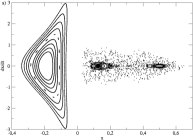
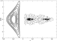
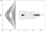
Figure 2: Poincare sections for a) the Newtonian system ($r_{S}^{*}=0$) , b) pseudo-Newtonian system with $r_{S}^{*}=5\times 10^{-10}$, c) $r_{S}^{*}=5\times 10^{-6}$ and d) $r_{S}^{*}=5\times 10^{-4}$. The figures a) and c) are very similar, and in d) it can be seen the formation of island chains around the stable region in the middle.

b) Lyapunov exponents

We shall study the Lyapunov exponents for the systems above described to better analyze the orbits stability. We shall use the Lyapunov characteristic number ($\lambda$) that is defined as the double limit

$$\lambda=\lim_{\scriptsize\begin{array}[]{l}\delta_{0}\rightarrow 0\\ t\rightarrow\infty\end{array}}\left[\log(\delta/\delta_{0})\over t\right],$$ (20)

where $\delta_{0}$ and $\delta$ are the deviation of two nearby orbits at times $0$  and $t$  respectively (see Alligood et al. [10]). We get the largest $\lambda$ using the technique suggested by Benettin et al. [11], in particular we use an algorithm due to Wolf et al. [12].

The Lyapunov exponents are not absolute, but dependent on the choice of the time scale. We recall that we have fixed the time scale by the requirement that $\omega=1$. This defines a time unit that is natural to each particular system. In these time units, for two different systems with equal Lyapunov exponents measured in inverse seconds and different angular frequencies $\omega_{1}$ and $\omega_{2}$ such that $\omega_{1}<\omega_{2}$, we will have that the system with larger frequency will have small Lyapunov exponent in the natural units of time, and vice versa. In other words, in this case, the separation of nearby orbits of the third body in each revolution of the first body will be larger for the system with smaller $\omega$. So we shall consider that, even though the two systems have equal Lyapunov exponents measured in inverse seconds the system with smaller angular frequency is more unstable that the one with larger $\omega$.

For $r_{S}^{*}=0$ we get $\lambda=0.185\pm 0.003$. The Lyapunov exponents for $r_{S}^{*}=4\times 10^{-12},5\times 10^{-10},5\times 10^{-8},5\times 10^{-6},5\times 10^{-4}$ are shown in the Fig. 3. We have a local minimum around $r_{S}^{*}=5\times 10^{-10}$.

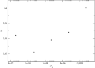
Figure 3: Lyapunov exponents for different values of $r_{S}^{*}$. Note that there is a minimum around $r_{S}^{*}=5\times 10^{-10}$.

c) Fractal escape and fractal dimension

Figure 4: Contour plot of the potential $U$ for the Newtonian system. For “energies” above $-2.16$ there are two escape routes, $x\rightarrow+\infty$ and $x\rightarrow-\infty$.

The Poincaré sections were obtained for values of the Jacobi constant such that the systems are bounded. For values larger than $C_{Jbounded}=-2.16$ the systems are unbounded and the third body escapes. In Fig. 4 we compute contour plot for the potential $U$ of the Newtonian system. The pseudo-Newtonian system is quite similar and will not be presented her. We see two escape routes, $x\rightarrow+\infty$ and $x\rightarrow-\infty$.

For open systems that have more than one route to escape we can apply the fractal escape technique used by Moura and Letelier [13] in the study of the classical Hénon-Heiles problem. In this method the basins of the escape routes are obtained for a set of initial conditions. For chaotic systems, we have the existence of fractal basin boundaries (FBB) indicating a great instability of the orbits. In our case we chose a subset of the accessible phase space at a fixed Jacobi constant, defined by a segment $|x|\leq a$, $y=b$ and $0\leq\theta\leq 2\pi$, where $a$ and $b$ are constants to be chosen appropriately and $\theta$ is the angle that defines the direction of the velocity with respect the $x$-axis. Then the trajectories are integrated numerically, we have three different cases: (1) the body escapes to $x\rightarrow+\infty$, (2) it escapes to $x\rightarrow-\infty$, and (3) the particle does not scape during the integration time. We take the integration time long enough to be sure that our results do not depend on this time. Fig. 5(a) shows the basins obtained for the Newtonian case. The pseudo-Newtonian basins are very similar and will not be shown here. In the figures, grey means initial conditions for particles that escape to $x\rightarrow+\infty$, black means that the particles escape to $x\rightarrow-\infty$ and white are the initial conditions for particles that do not escape. A zoom of a portion of 5(a) is shown in Fig. 5(b), we see self-similarity of the basin boundaries, a fractal characteristic.

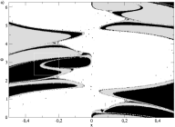
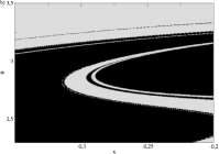
Figure 5: (a) Escape basins for the Newtonian system. Grey (black) means initial conditions for particles that escape to $x\rightarrow+\infty$ ( $x\rightarrow-\infty$) and white are the initial conditions for particles that do not escape during the integration time. (b) A zoom of the portion of the precedent figure enclosed by the square.

To show the diference between systems with different values of the parameter $r_{S}^{*}$, we calculate the dimension of the basin boundaries obtained for the different systems. The dimension used is the box-counting dimension that can be easily obtained, see for instance, Ott [14] and Grebogi et al. [15]. If we displace a determined point of a basin to another on a distance $\epsilon$, the probability that this new initial condition does not belong to the same basin of the old one is, for small $\epsilon$, $P(\epsilon)\propto\epsilon^{D-d}$, where $D$ is the dimension of the set ($2$ in our case) and $d$ is the box counting dimension, also called exterior or fractal dimension when not integer. In order to calculate this fractal dimension, for several values of $\epsilon$, we displace the $x$ coordinate of all the points from one of the basins ($x\rightarrow+\infty$), and count the number of points that does not belong to the same basin. Then we compute the the fraction of numbers that does not belong to the same basin, $P(\epsilon)$. We plot $\ln P(\epsilon)$ in function of $\ln\epsilon$. The inclination of the straight line gives us $D-d$. The obtained values for the fractal dimension, $d$, are shown in the Table 1. Some of the values obtained are indistinguishable one from each other in the precision used. Due to his high instability, we were not able to calculate the fractal dimension of the $r_{S}^{*}=4\times 10^{-4}$ system. This value is probably near $2$, the higher value.

Table 1: Fractal dimensions for Newtonian and pseudo-Newtonian systems

$r_{S}^{*}$	Fractal Dimension
$0$ (Newtonian system)	$1.452\pm 0.003$
$4\times 10^{-12}$	$1.451\pm 0.003$
$5\times 10^{-10}$	$1.452\pm 0.003$
$5\times 10^{-8}$	$1.459\pm 0.003$
$5\times 10^{-6}$	$1.466\pm 0.003$

5 Conclusions

We can see directly from the Lyapunov exponents and confirmed by the Poincaré sections that the pseudo-Newtonian systems (a relativistic simulation) are not always more unstable than their equivalent Newtonian systems.

It could be guessed a priori that the pseudo-Newtonian systems should be more unstable due to the fact that the Paczynski-Wiita potential introduces a saddle point in the dynamical system. However this happens only for $r_{S}^{*}>(9/4)^{1/3}\approx 1.31$. As we mention before, due to the approximation used for the Hill problem, we have $r_{S}^{*}<0.63$. Thus in the cases under consideration the number of saddle points is the same for both Newtonian and pseudo-Newtonian systems. Another feature is the presence of a local minimum for the Lyapunov exponents, indicating that there exists a more stable configuration for pseudo-Newtonian systems that is even more stable than the equivalent Newtonian configuration. This minimum corresponds to a known physical system, the Milky Way-M2-star system. This is an evidence that relativistic effects can made a system more stable. This is related to the fact that the addition of extra spherical terms in the Newtonian potential can be used to damp the influence of the non-spherical perturbation, making the motion more regular, see, for instance, Ivanov et al. [16]. This needs to be confirmed by a fully General Relativistic treatment of the Hill problem. We hope to comeback to this subject soon.

6 Acknowledgements

We want to thank CNPq and FAPESP for financial suport.

References

- [1] G.W. Hill, Am. J. Math. 1 (1878) 129.
- [2] D. Heggie, in: B.A. Steves, A.J. Maciejewski (Eds.), The Restless Universe, Scottish Universities Summer School in Physics and Institute of Physics Publishing, Bristol, 2001, p. 109.
- [3] E. Meletlidou, S. Ichtiroglou, F.J. Winterberg, Celest. Mech. Dynam. Astron. 80 (2001) 145.
- [4] C. Simó, T.J. Stuchi, Physica D 140 (2000) 1.
- [5] B. Paczyński, P. Wiita, Astron. Astrophys. 88 (1980) 23.
- [6] C.D. Murray, S.F. Dermott, Solar System Dynamics, Cambridge Univ. Press, Cambridge, 1999.
- [7] V.I. Arnold, Mathematical Aspects of Classical and Celestial Mechanics, Springer-Verlag, Berlin, 1997, p. 88.
- [8] E. Guéron, P.S. Letelier, Astron. Astrophys. 368 (2001) 716.
- [9] O. Semerák, V. Karas V. Astron. Astrophys. 343 (1999) 325.
- [10] K. Alligood, T. Sauer, J. Yorke, Chaos - An Introduction to Dynamical Systems, Springer-Verlag, Berlin, 1996, p. 203.
- [11] G. Benettin, L. Galgani, A. Giorgilli, J.W. Strelcyn, Meccanica 15 (1980) 9.
- [12] A. Wolf, J.B. Swift, H.L. Swinney, J.A. Vastano, Physica D 16 (1985) 285.
- [13] A.P.S. Moura, P.S. Letelier, Phys. Lett. A 256 (1999) 362.
- [14] E. Ott, Chaos in Dynamical Systems, Cambridge University Press, Cambridge, 1993.
- [15] C. Grebogi, H.E. Nusse, E. Ott, J.A. Yorke, in: J.C. Alexander (Ed.), Dynamical Systems, Springer-Verlag, Berlin, 1988, p. 220.
- [16] P.B. Ivanov, A.G. Polnarev, P. Saha, Mon. Not. R. Astron. Soc. 358 (2005) 1361.