SWIFT XRT OBSERVATIONS OF THE AFTERGLOW OF XRF 050416A

Abstract

Swift discovered XRF 050416A with the Burst Alert Telescope and began observing it with its narrow field instruments only 64.5 s after the burst onset. Its very soft spectrum classifies this event as an X-Ray Flash. The afterglow X-ray emission was monitored up to 74 days after the burst. The X-ray light curve initially decays very fast (decay slope $\alpha\sim 2.4$), subsequently flattens ($\alpha\sim 0.44$) and eventually steepens again ($\alpha\sim 0.88$), similar to many X-ray afterglows. The first and second phases end $\sim 172$ and $\sim 1450$ s after the burst onset, respectively. We find evidence of spectral evolution from a softer emission with photon index $\Gamma\sim 3.0$ during the initial steep decay, to a harder emission with $\Gamma\sim 2.0$ during the following evolutionary phases. The spectra show intrinsic absorption in the host galaxy with column density of $\sim 6.8\times 10^{21}$ cm^-2. The consistency of the initial photon index with the high energy BAT photon index suggests that the initial fast decaying phase of the X-ray light curve may be the low-energy tail of the prompt emission. The lack of jet break signatures in the X-ray afterglow light curve is not consistent with empirical relations between the source rest-frame peak energy and the collimation-corrected energy of the burst. The standard uniform jet model can give a possible description of the XRF 050416A X-ray afterglow for an opening angle larger than a few tens of degrees, although numerical simulations show that the late time decay is slightly flatter than expected from on-axis viewing of a uniform jet. A structured Gaussian-type jet model with uniform Lorentz factor distribution and viewing angle outside the Gaussian core is another possibility, although a full agreement with data is not achieved with the numerical models explored.

1. INTRODUCTION

The Swift Gamma-Ray Burst Explorer (Gehrels et al., 2004), successfully launched on 2004 November 20, is dedicated to the discovery and study of gamma-ray bursts (GRBs) and their X-ray and optical afterglows. Its fast-pointing capability, compared with previous satellites, allows us to repoint towards GRB sources approximately 100 s after the burst detection by the Burst Alert Telescope (BAT; Barthelmy et al., 2005a) and to study, for the first time, the early phases of the afterglow evolution. Moreover, the very broad energy coverage allows a simultaneous study of the phenomenon in the optical, soft and hard X-ray bands.

One of the main Swift results has been the direct observation of the transition between the prompt and the afterglow emission. A growing number of early rapidly-fading X-ray afterglows have been observed by Swift, that have been successfully interpreted as the tail of the prompt GRB emission (e.g. Tagliaferri et al., 2005; Cusumano et al., 2006a; Barthelmy et al., 2005b; Nousek et al., 2006; Chincarini et al., 2005; Zhang et al., 2006). The emergence of the true X-ray afterglow component has been identified with a break in the X-ray light curve to a less steep (often flat) decay rate, sometimes accompanied by spectral variation across the break. Further breaks in the X-ray light curve have been related to standard afterglow evolution. The light curve of the X-ray counterpart of XRF 050416A show all these characteristic features.

BAT detected and located XRF 050416A on 2005 April 16, 11:04:44.5 UT, at the coordinates RA${}_{\rm J2000}=12^{\rm h}33^{\rm m}57\fs 6$, Dec${}_{\rm J2000}=+21\arcdeg 03\arcmin 10\farcs 8$, with an uncertainty of 3$\arcmin$ (Sakamoto et al., 2005a, b). The light curve showed a single peak followed by a small bump with duration $T_{90}$=2.4$\pm 0.2$ s, with most of the energy emitted in the $15-50$ keV band. The time-averaged energy distribution was well described by a power law ($N(E)\propto E^{-\Gamma}$) with photon index $\Gamma=3.1\pm 0.2$ (90% confidence level) (Sakamoto et al., 2005c). The soft spectrum and the fact that the fluence in the $15-30$ keV energy band is $6.1\times 10^{-7}$ erg cm^-2, larger than the fluence in the $30-400$ keV band ($1.3\times 10^{-7}$ erg cm^-2) classify this event as an X-ray flash (XRF; Heise et al., 2001; Lamb et al., 2005). A complete ground analysis of the BAT data is presented in Sakamoto et al. (2005c). These authors found that the best fit for the average energy distribution of the burst over the $T_{90}$ interval is given by a Band model (Band et al., 1993), with peak energy $E_{\rm p}=15.6^{+2.3}_{-2.7}$ keV, low-energy spectral slope $\alpha_{\rm Band}=-1$ (fixed) and high-energy slope $\beta_{\rm Band}<-3.4$ (68% confidence level). This represents a 3.1 $\sigma$ improvement with respect to a simple power law fit ($\Gamma=3.1\pm 0.2$ over the 14$-$150 keV energy band). Sakamoto et al. (2005c) also showed that spectral hard-to-soft evolution was present during the BAT observation, with the spectrum becoming considerably softer at the end of each peak, and estimated an isotropic energy $E_{\rm iso}\sim 1.2\times 10^{51}$ erg.

Following the burst detection, the satellite executed an immediate slew and promptly began collecting data at 11:05:49 UT (64.5 s after the trigger) with the Ultraviolet/Optical Telescope (UVOT; Roming et al., 2005) and at 11:06:00.6 UT (i.e. 76.1 s after the trigger) with the X-Ray Telescope (XRT; Burrows et al., 2005a).

In the first 100 s of observation UVOT revealed a new source in the $V$ filter at RA${}_{\rm J2000}=12^{\rm h}33^{\rm m}54\fs 56$, Dec${}_{\rm J2000}=+21\arcdeg 03\arcmin 27\farcs 3$ (with an uncertainty radius of $0\farcs 56$ (Holland et al., 2006)), with magnitude $V=19.38$ (Schady et al., 2005a). Starting with data taken 207 s after the trigger, the source was also detected in the $U$ and $B$ bands, with magnitudes $U=19.34\pm 0.20$ and $B=19.85\pm 0.20$ mag. There was no further detection in the $V$ band down to the 5 $\sigma$ limiting magnitude of 19.57 mag (Schady et al., 2005b), 173 s after the first $V$-band image. A fading source was also detected at 193 nm (UVW2 filter), placing an upper limit of 1 to the GRB redshift (Fox, 2005). The results and implications of the UVOT observations are discussed in Holland et al. (2006).

Ground-based optical, NIR, and radio follow-up observations were performed with several instruments. A fading source was detected with the ANU 2.3 m telescope in the $R$ band (Anderson et al., 2005), with the Palomar 200-inch Hale Telescope in the $K_{\rm s}$ band $\sim 6$ min after the BAT trigger (Cenko et al., 2005a), with the MAO telescope in the $R$ band ($R=20.85\pm 0.12$, with a 900 s exposure, 11 hr after the trigger; Kahharov et al., 2005), and, marginally, with the KAIT in a 60 s $I$-band image, 7.4 min after the trigger (Li et al., 2005). A late observation performed with the MAGNUM telescope equipped with the MIP dual-beam optical-NIR imager detected the afterglow with $R=21.3$ mag, 12.2 hr after the trigger. Spectra of the host galaxy of XRF 050416A were taken with the Low Resolution Imaging Spectrometer mounted on the 10-m Keck I telescope (Cenko et al., 2005b). The spectrum indicates that the host galaxy is faint and blue with a large amount of ongoing star formation. Spectral analysis revealed several emission lines including [OII], H$\beta$, H$\gamma$, and H$\delta$, at a redshift $z=0.6535\pm 0.0002$. This is consistent with the prediction of Fox (2005) based on the afterglow detection in the Swift UVOT UVW2 filter. XRF 050416A is thus one of the closest long GRBs discovered by Swift.

At radio frequencies, no source was detected with the VLA down to a limiting flux of 260 $\mu$Jy at 8.46 GHz 37 min after the burst (Frail & Soderberg, 2005) or with the Giant Meter-wave Radio Telescope at 1280 MHz $\sim 9$ d after the burst (placing an upper limit of 94 $\mu$Jy; Ishwara-Chandra et al., 2005), while a source with flux density $260\pm 55~{}\mu$Jy was detected with the VLA at 4.86 GHz, 5.6 d after the burst (Soderberg, 2005).

In the following, we report on the analysis of the prompt emission and of the X-ray afterglow observed by Swift. Details on the follow-up XRT observations and the XRT data reduction are described in § 2; the temporal and spectral analysis results are reported in § 3. In § 4 we discuss our results. Conclusions are drawn in § 5. Finally, in the Appendix we will show how our interpretation of the early XRT light curve as the tail of the prompt emission could be reconciled with the report of a peak energy $E_{\rm p}=15.6^{+2.3}_{-2.7}$ keV by Sakamoto et al. (2005c) and the observed hardness evolution of the BAT light curve.

Throughout this paper the quoted uncertainties are given at the 90% confidence level for one interesting parameter, unless otherwise specified. We also adopt the notation $F(\nu,t)\propto t^{-\alpha}\nu^{-\beta}$ for the afterglow monochromatic flux as a function of time, with $\nu$ representing the frequency of the observed radiation and with the energy index $\beta$ related to the photon index $\Gamma$ according to $\beta=\Gamma-1$.

Table 1XRT observation log of XRF 050416A

Obs. #	Sequence	Mode	Start time (UT)	Start time	Exposure
			(yyyy-mm-dd hh:mm:ss.s)	(s since trigger)	(s)
1	00114753000	LR	2005-04-16 11:05:49.0	64.5	8.2
1	00114753000	IM	2005-04-16 11:06:00.6	76.1	2.5
1	00114753000	WT	2005-04-16 11:06:08.6	84.1	9.6
1	00114753000	PC	2005-04-16 11:06:18.2	93.8	57360
2	00114753001	PC	2005-04-18 14:27:56.9	184992.4	35084
3	00114753003	PC	2005-04-26 00:53:32.7	827328.2	21279
4	00114753004	PC	2005-04-28 01:07:03.8	1000939.3	20710
5	00114753005	PC	2005-05-02 00:24:42.2	1343997.7	6892
6	00114753006	PC	2005-05-03 00:33:40.8	1430936.3	5696
7	00114753008	PC	2005-05-08 16:38:29.5	1920825.0	16702
8	00114753009	PC	2005-05-13 01:08:16.3	2297011.8	22628
9	00114753010	PC	2005-05-14 01:13:22.3	2383717.8	29625
10	00114753011	PC	2005-05-25 04:03:25.2	3344320.7	23897
11	00114753012	PC	2005-05-26 02:50:04.0	3426320.5	692
12	00114753013	PC	2005-05-27 01:06:28.8	3506504.3	5077
13	00114753014	PC	2005-05-29 01:18:21.3	3680016.8	19254
14	00114753018	PC	2005-06-21 00:46:21.1	5665296.6	27979
15	00114753019	PC	2005-06-22 00:46:54.2	5751729.7	24071
16	00114753020	PC	2005-06-23 00:55:53.8	5838669.3	24073
17	00114753021	PC	2005-06-25 01:07:54.8	6012190.3	14581
18	00114753022	PC	2005-06-28 00:04:59.1	6267614.6	13215
19	00114753023	PC	2005-06-29 00:05:00.2	6354015.7	11435

2. XRT OBSERVATIONS AND DATA REDUCTION

The Swift XRT is designed to perform automated observations of newly discovered bursts in the $0.2-10$ keV band. Four different read-out modes have been implemented, each dependent on the count rate of the observed sky region. The transition between two modes is automatically performed on board (see Hill et al., 2004, 2005a for a detailed description of XRT observing modes).

XRT was on target 76.1 s after the BAT trigger. It was operating in auto state and went through the standard sequence of observing modes, slewing to the GRB field of view in Low Rate Photodiode (LR) mode, taking a 2.5 s frame in Image (IM) mode followed by a LR frame (1.3 s), and 8 Windowed Timing (WT) mode frames (9.6 s), and then correctly switching to Photon Counting (PC) mode for the rest of the orbit. XRT was not able to automatically detect the source centroid on-board because of its low intensity, but ground analysis revealed a fading object identified as the X-ray counterpart of XRF 050416A (Cusumano et al., 2005). XRF 050416A was then observed intermittently over 29 consecutive orbits for a total exposure time of 57 454 s. During the 8th orbit (starting $\sim 35$ ks after the trigger), the brightening of a column of flickering pixels caused uncontrolled mode-switching between WT and PC modes. The WT data from this orbit are not usable because of their very low signal to noise (S/N) ratio. XRF 050416A was further observed several times up to 74 d later in PC mode. The observation log is presented in Table 1.

XRT data were downloaded from the Swift Data Center at NASA/GSFC (level 1 data products). They were then calibrated, filtered, and screened using the XRTDAS software package (v.2.3) developed at the ASI Science Data Center (ASDC) to produce cleaned photon list files. The temperature of the CCD was acceptably below $-50$ °C for the whole observation set. The total exposure times after all the cleaning procedures were 8.2 s, 9.6 s, and 368 815 s for data accumulated in LR, WT, and PC mode, respectively.

For both the spectral and timing analyses we used standard grade selections: $0-12$ for PC mode, $0-5$ for LR mode, and $0-2$ for WT mode. However, data in WT mode had insufficient statistics to allow for detailed spectral modeling and were used only in the light curve analysis. Ancillary response files for PC and LR spectra were generated through the standard xrtmkarf task (v0.5.1) using the response files swxpc0to12_20010101v007.rmf and swxpd0to5_20010101v007.rmf from CALDB (2006-01-04 release).

In the timing analysis, XRT times are referred to the XRF 050416A BAT trigger time $T=2005$ Apr 16.461626 UT (2005 Apr 16, 11:04:44.5 UT).

3. XRT DATA ANALYSIS

3.1. SPATIAL ANALYSIS

Figure 1 (left panel) shows the XRT image accumulated in PC mode with a $0.2-10$ keV energy selection during the first and second observations, together with the BAT and XRT error circles. The central portion of this field is expanded in the right panel of Fig. 1, in which we show the cumulative image of the follow-up observations # 3 to 13. Two sources are visible within the BAT error circle. The brighter one is coincident with the position of the optical counterpart as derived by UVOT (cross point) and it is clearly fading with time. Therefore we identify it as the afterglow of XRF 050416A. The fainter source lies 21$\farcs$6 away from the UVOT afterglow (Schady et al., 2005a) and it does not show any significant evidence of intensity variations during the XRT observations. Its count rate, as determined from the sum of the follow-up observations # 3 to 13 (chosen to minimize the contamination from the afterglow emission) is $(3.3\pm 0.7)\times 10^{-4}$ count s^-1.

The afterglow position derived with xrtcentroid (v0.2.7) is RA${}_{\rm J2000}=12^{\rm h}33^{\rm m}54\fs 62$, Dec${}_{\rm J2000}=+21\arcdeg 03\arcmin 27\farcs 7$, with an uncertainty of 3$\farcs$3. This position takes into account the correction for the misalignment between the telescope and the satellite optical axis (Moretti et al., 2006). The XRT boresight corrected coordinates are 45$\farcs$0 from the BAT position (Sakamoto et al., 2005b) and 0$\farcs$9 from the optical counterpart (Schady et al., 2005a).

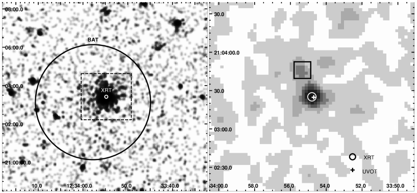
Figure 1.— Left: Photon Counting mode XRT image of the first and second observations (92 ks exposure), smoothed with a Gaussian filter with a 3 pixel standard deviation, showing the XRT and BAT error circles (Moretti et al., 2006, Sakamoto et al., 2005b, respectively). The dashed box identifies the area enlarged in the right panel. The UVOT afterglow position is not marked on this image because it is indistinguishable from the XRT one. Right: Cumulative image of the follow-up observations from 3 to 13 (152 ks exposure; Table 1), showing the XRT error circle, the UVOT position as given in Schady et al. (2005a) (cross) and the position of the second source detected within the BAT error circle (square).

Figure 2.— BAT and XRT light curves of XRF 050416A. The XRT count rate ($0.2-10$ keV) was converted into flux units by applying a conversion factor derived from the spectral analysis. The solid line represents the best-fit model with the doubly-broken power law. The dashed line is the extrapolation of the XRT best fit model prior to the first XRT observation. The BAT light curve was extrapolated into the $0.2-10$ keV XRT energy band by converting the $15-150$ keV BAT count rate through the single power law best fit model with photon index $\Gamma=3.1$ presented in Sakamoto et al. (2005c).

3.2. TIMING ANALYSIS

The X-ray emission from the counterpart of XRF 050416A was detected for the first time in the settling data (i.e. those data collected during the satellite slew, when the XRT pointing direction was less than 10′ off the target position). We have a total of 8.2 s of data in which the source is significantly detected before the “official” beginning of the pointed XRT observation. In these data the maximum offset of the source is lower than 3$\arcmin$ and no vignetting correction was thus required. As LR is a non-imaging mode, the background has been extracted from pointed LR data taken at the beginning of an orbit, $1.5\times 10^{5}$ s after the burst trigger, when, as we know from the PC data (see below), the afterglow emission had faded to less than 1% of the initial value. This background subtraction allows us to correctly account for the emission of the serendipitous non-transient sources in the field of view in addition to the instrumental and cosmic X-ray background.

After settling, a single exposure (2.5 s) image mode frame was taken, which officially marks the beginning of pointed observation. We determined the total amount of charge above the background inside a circular region of 30 pixel radius centered at the source position in raw telemetry units (i.e. Data Number or DN units). We obtained 278 DN above a background of 0.5 DN. The DN value was converted to count rate by evaluating the mean energy of the LR spectrum in the $0.2-10$ keV band (1490 eV). Given a mean energy per DN of $\sim$79 eV in the low gain imaging mode we calculated a rate of $5.9\pm 1.5$ count s^-1.

WT data were extracted in a rectangular region 40 pixels wide along the image strip, which includes about 98% of the point spread function (PSF). The background level was extracted from a rectangular region of the same extension, far from the source and affected by minimal contamination from other sources in the field. The rapid decay of the source and the high background level in WT mode allow us to have a significant detection of the XRF 050416A only in the first 8 frames (9.6 s) of the WT data set.

Given the pile-up effect in the first part of the observation, the presence of the second source and the weakness of the afterglow after the first follow-up observation, the PC data require different extraction regions for different rate levels, in order to optimize the S/N ratio.
First orbit. The intensity of the source during the first orbit of the first observation (Table 1) was high enough to cause pile-up in the PC frames. In order to correct for this effect, we extracted counts from an annular region with an outer radius of 30 pixels (70$\farcs$8) and an inner radius of 3 pixels (7$\farcs$1). Such a region includes about 52% of the PSF. The optimal inner radius was evaluated by comparing the analytical PSF with the profile extracted in the first 2000 s of observation. The excluded region corresponds to pixels deviating more than one sigma from the best fit of the differential PSF wings (i.e. the fit performed on data from 7 pixels outwards). The light curve was corrected for the PSF fraction loss.
First observation (excluding the first orbit) and second observation. In the following 28 orbits of the first observation and throughout the second observation the intensity of the afterglow was lower than 0.1 count s^-1 and the pile-up was negligible. The data were extracted from the entire circular region of 30 pixels radius in order to have the maximum available statistics, particularly important in the last part of the afterglow decay. This circle encloses 93% of the PSF. Both here and in the previous case, the contribution of the second, fainter source detected within the BAT error box is negligible with respect to the afterglow intensity.
Observations 3 to 13. The afterglow had faded to a count rate comparable to that of the serendipitous source. In order to avoid significant (i.e. greater than 10%) contamination, we reduced the extraction radius to 6.5 pixels (15$\arcsec$). Such a region includes about 71% of the source PSF and the possible contamination from the nearby source within this region amounts to about 12% of its PSF. Given the faintness of the afterglow in this final part of the light-curve, this choice also improves the S/N ratio.

The background level for the PC data was extracted in an annular region with an inner radius of 40 pixels and an outer radius of 150 pixels centered at the source position. To eliminate contributions from faint sources in the background region, we produced a 380 ks image by summing all of the observations, and searched this image for faint sources within the background annulus. In addition to the serendipitous source shown in Fig. 1, 20 other sources were found with S/N ratio higher than 3, all of which were located more than 50 pixels from the afterglow. The contributions from these sources were excluded from the background region.

Data were binned in order to have a S/N ratio higher than 3. The source was not detectable after observation # 13; data from observations 14-19 were summed together and provide a single 3 $\sigma$ upper limit value of $2.3\times 10^{-4}$ count s^-1. Figure 2 shows the background-subtracted light curve in the $0.2-10$ keV energy band. The source is clearly fading with time.

The XRT light curve decay is not consistent with a single power law ($\chi_{\rm red}^{2}=1.43$, with 80 degrees of freedom, d.o.f.). A broken power law:

$$F(t)=\left\{\begin{array}[]{ll}K~{}t^{-\alpha_{\rm A}}&\textrm{ {\rm for}~{} $t<T_{\rm b}$ }\\ K~{}T_{\rm b}^{\alpha_{\rm B}-\alpha_{\rm A}}t^{-\alpha_{\rm B}}&\textrm{ {\rm for}~{} $t\geq T_{\rm b}$ }\\ \end{array}\right.$$

(where $\alpha_{\rm A}$ and $\alpha_{\rm B}$ are the power-law slopes before and after the break time $T_{\rm b}$, respectively) improves the fit, giving $\chi_{\rm red}^{2}=1.20$ (78 d.o.f.). However, the residuals show a systematic trend. Adding a second break to the model:

$$F(t)=\left\{\begin{array}[]{ll}K~{}t^{-\alpha_{\rm A}}&\textrm{ {\rm for}~{} $t<T_{\rm b,1}$ }\\ K~{}T_{\rm b,1}^{\alpha_{\rm B}-\alpha_{\rm A}}~{}t^{-\alpha_{\rm B}}&\textrm{ {\rm for}~{} $T_{\rm b,1}\leq t<T_{\rm b,2}$ }\\ K~{}T_{\rm b,1}^{\alpha_{\rm B}-\alpha_{\rm A}}~{}T_{\rm b,2}^{\alpha_{\rm C}-\alpha_{\rm B}}~{}t^{-\alpha_{\rm C}}&\textrm{ {\rm for}~{} $t\geq T_{\rm b,2}$ }\\ \end{array}\right.$$

the fit further improves yielding $\chi_{\rm red}^{2}=0.81$ (76 d.o.f.). The F-test for this model vs. the simple broken power-law gives a chance probability of $1.2\times 10^{-7}$. This last model reveals the presence of two breaks at $172\pm 36$ s and at (1.450 $\pm$ 0.013) $\times 10^{3}$ s. Table 2 shows the best fit results obtained with the three models. We also tried to fit the light curve with a single or broken power law allowing the reference time $t_{0}$ to be a free parameter. For the simple power law and the single break broken power-law $\chi^{2}_{\rm red}$ improved to 1.40 (79 d.o.f.) and 1.02 (77 d.o.f.), respectively, but the best-fit model is not able to account for the initial part of the light curve decay and the resulting $t_{0}$ is before the burst onset ($t_{0}=-201\pm 156$ s and $t_{0}=-153\pm 34$ s, respectively). For the doubly-broken power law the improvement is not significant and the value of $t_{0}$ is marginally consistent with the burst trigger time.

In Fig. 2 we plot the data as well as the best fit model obtained with the doubly-broken power law, with $t_{0}=0$. We also show the model extrapolation back to the time of the trigger. Hereafter, we will refer to the time intervals $t<T_{\rm b,1}$, $T_{\rm b,1}<t<T_{\rm b,2}$, and $t>T_{\rm b,2}$ as phases ‘A’, ‘B’, and ‘C’, respectively.

Note that the second observation starts after the second break in the light curve (see fifth column in Table 1), and all other observations contribute only to phase C. Observations from 3 to 13 correspond to the last seven points of the light curve shown in Fig. 2, and observations from 14 to 19 give the final upper limit.

Table 2XRF 050416A light curve best fit parameters

Parameter	Single PL	Broken PL	Doubly-broken PL
$\alpha_{\rm A}$	0.82 $\pm$ 0.02	3.28 $\pm$ 0.04	2.4 $\pm$0.5
$T_{\rm b,1}$ (s)	–	103 $\pm$ 9	172 $\pm$ 36
$\alpha_{\rm B}$	–	0.81 $\pm$ 0.02	0.44 $\pm$ 0.13
$T_{\rm b,2}$ (103 s)	–	–	1.450 $\pm$ 0.013
$\alpha_{\rm C}$	–	–	0.88 $\pm$ 0.02
$\chi_{\rm red}^{2}$ (d.o.f.)	1.43 (80)	1.20 (78)	0.81 (76)

Note. — $\alpha_{\rm A}$, $\alpha_{\rm B}$, and $\alpha_{\rm C}$ are the decay slopes for the distinct phases of the light curve (see § 3.2). $T_{\rm b,1}$ and $T_{\rm b,2}$ are the epochs at which the decay slope changes, measured from the XRF onset. The IM and LR points have been included in the fits.

Figure 3.— Phase A, B, and C spectra converted in the $E^{2}N(E)$ (or $\nu F_{\nu}$) representation together with their best fit absorbed power-law models. The panels showing residuals refer to phase A, B, and C, respectively from top to bottom.

3.3. SPECTRAL ANALYSIS

Detailed spectral analysis could be performed only for the LR data in settling mode acquired before the start of the first observation and on the PC data of the first and second observations; the following 11 observations did not add significant statistics to the spectra, thus they were not included in the analysis. The same holds for the WT data of the first observation consisting of only 31 (background-subtracted) photons.

Given the presence of three different phases in the XRF 050416A light curve decay, we first checked for spectral variability during the afterglow evolution. The LR spectrum and background were extracted as described in § 3.2. The two PC spectra for the phases A and B in Fig. 2 were extracted from the first observation with the same annular region used for the timing analysis, while the PC spectrum for the phase C was extracted from the remaining part of the first observation and the second observation (i.e. up to $2.8\times 10^{5}$ s) using the circular region of 30 pixel radius. The PC background spectra were extracted from the same region as for the timing analysis.

We fitted the spectra from phases A, B, and C separately with absorbed power laws. For phase A, the LR and PC spectra were fitted together leaving the normalization parameters free to take into account the different rate level due to the light curve decay. The four spectra are shown in Fig. 3 together with their absorbed power law best fits.

The best fit results show evidence for spectral variation among phases: the emission in phase A is significantly softer than in the phases B and C. In the latter two phases the best fit photon indices were consistent within the errors. Spectra extracted from phases B and C were, therefore, summed together and their ancillary response files, obtained from different extraction regions, were weighted according to the relative exposure. The fit of the resulting spectrum gave an absorption column density of $(2.6^{+0.4}_{-0.3})\times 10^{21}$ cm^-2 and a photon index $\Gamma=2.04_{-0.05}^{+0.11}$, with a reduced $\chi^{2}$ of 1.2 (83 d.o.f.). The observed column density is significantly larger than the Galactic value ($0.21\times 10^{21}$ cm^-2). We therefore checked for intrinsic absorption in the host galaxy by adding a redshifted absorption component (zwabs model in XSPEC v11.3.1) with the redshift fixed to 0.6535 (Cenko et al., 2005b) and the Galactic absorption column fixed to $0.21\times 10^{21}$ cm^-2. The fit gave a value of $6.8^{+1.0}_{-1.2}\times 10^{21}$ cm^-2 for the additional column density with an improvement of the reduced $\chi^{2}$ to 1.0 (83 d.o.f.). The phase A spectra, that also showed a column density significantly higher than the Galactic value, were fitted again with the addition of a redshifted absorption component. Because of the low statistics of the phase A data, the column density was kept fixed to the value obtained from the phase B$+$C spectral fit and the best fit photon index was $\Gamma=3.0^{+0.3}_{-0.4}$ ($\chi^{2}_{\rm red}=0.6$; 5 d.o.f.). Table 3 shows the final results of the spectral analysis.

Table 3XRF 050416A XRT spectral fit results

Parameter	Phase A	Phase B+C
Galactic column density ($10^{21}~{}{\rm cm}^{-2}$)	0.21 (frozen)	0.21 (frozen)
Host column density ($10^{21}~{}{\rm cm}^{-2}$)	6.8 (frozen)	$6.8^{+1.0}_{-1.2}$
Photon index	$3.0^{+0.3}_{-0.4}$	$2.04^{+0.11}_{-0.05}$
$N$ (photons keV-1 cm-2 s-1 at 1 keV)	$0.14\pm 0.03$	$(2.7\pm 0.3)\times 10^{-4}$
$0.2-10$ keV flux (erg cm-2 s-1)	($1.9\pm 0.1)\times 10^{-10}$	$(1.7\pm 0.2)\times 10^{-12}$
$0.2-10$ keV luminosity (erg s-1)	$5.7\times 10^{47}$	$3.1\times 10^{45}$
$\chi_{\rm red}^{2}$ (d.o.f.)	0.6 (5)	1.0 (83)

Note. — The intrinsic column density for the LR data was held fixed to the best fit value found from the PC spectrum. The (isotropic) luminosity was calculated for a redshift $z=0.6535$, with $H_{0}$=70 km s^-1 Mpc^-1, $\Omega_{\rm m}$=0.3, and $\Omega_{\Lambda}$=0.7. Unabsorbed fluxes and luminosities reported for the PC data are averaged over long time intervals: accurate instantaneous values for the unabsorbed flux can be derived from Fig. 2.

4. DISCUSSION

We have presented a detailed analysis of the X-ray afterglow of XRF 050416A. The prompt emission of this burst lasts $\sim 2.5$ s and is characterized by a first peak followed by a second much weaker one. The event belongs to the short tail of the long GRB population (Kouveliotou et al., 1993). It could also be consistent with the third class of bursts identified by Mukherjee et al. (1998) through multivariate analysis on the BATSE catalog. This class consists of bursts of intermediate duration and fluence as compared to the standard classes of short/faint/hard and long/bright/soft GRBs. The average energy distribution of the prompt emission is soft (well fitted by a power law with $\beta=\Gamma-1=2.1\pm 0.2$ at the 90% confidence level or by a Band model with $\alpha_{\rm Band}\equiv-1$, $E_{\rm p}=15.6_{-2.7}^{+2.3}$ keV, and $\beta_{\rm Band}<-3.4$ at the 68% confidence level) with significant evidence of hard to soft evolution within each peak (Sakamoto et al., 2005c). The gamma-ray spectral distribution of this burst, with fluence in the X-ray energy band $2-30$ keV larger than the fluence in $30-400$ keV band, classifies it as an X-ray flash (Lamb et al., 2005; Sakamoto et al., 2005d).

XRT monitored the XRF 050416A X-ray emission from $\sim 64.5$ s up to 74 d after the BAT trigger. XRF afterglows have been rarely detected in the past (XRF 011030, XRF 020427: Bloom et al., 2003; Levan et al., 2005a; XRF 030723: Butler et al., 2005; XRF 040701: Fox, 2004; XRF 050215B: Levan et al., 2005b; XRF 050315: Vaughan et al., 2006; XRF 050406: Burrows et al., 2005b; Romano et al., 2006a; XRF 050824: Krimm et al., 2005). The exceptionally long observational campaign of XRF 050416A has provided us with a unique data set and allowed one of the most accurate spectral and timing analyses ever performed for an XRF afterglow.

The XRF 050416A light curve of the first $10^{5}$ s after the trigger (Fig. 2) is fairly smooth and similar in shape to other Swift-detected XRF and GRB afterglows like XRF 050315 (Vaughan et al., 2006) or GRB 050319 (Cusumano et al., 2006a; see also Nousek et al., 2006; Chincarini et al., 2005; O’Brien et al., 2006). It shows evidence of three different phases (A, B, and C according to § 3.2), each of them characterized by a distinct decay slope (see Fig. 2 and Table 2). At the beginning of the XRT observation the light curve shows a steep decay ($\alpha_{\rm A}\sim 2.4$), followed by a short flat phase ($\alpha_{\rm B}\sim 0.44$) and then by a third long-lasting phase with a more rapid intensity decline ($\alpha_{\rm C}\sim 0.9$). We also found that the late extrapolation of the phase C decay is consistent with the flux upper limit measured $65-74$ d after the prompt emission (observations # $14-19$). There is no evidence of X-ray flares as seen in XRF 050406 (Romano et al., 2006a), GRB 050502B (Burrows et al., 2005b; Falcone, 2006), GRB 050607 (Pagani et al., 2006), and many other events.

The XRT spectra show significant excess absorption in the rest frame of XRF 050416A ($N_{\rm H}\sim 6.8\times 10^{21}$ cm^-2) and an energy distribution significantly softer in phase A ($\beta=2.0\pm 0.4$) than in phases B and C, which have consistent spectral slope with a weighted average energy index $\beta=1.04\pm 0.05$. This may indicate a different emission process acting during the initial phase of the XRF 050416A light curve.

4.1. PHASE A

In the internal/external shock scenario (Rees & Mészáros, 1994), the tails of GRB peaks are expected to be caused by the “high latitude effect” (Kumar & Panaitescu, 2000; Dermer, 2004). If a relativistic shell of matter suddenly stops shining, a distant observer receives photons emitted from increasing off-axis angles at later times due to the longer travel path. When the observed frequency is above the synchrotron cooling frequency (which is usually the case in the X-ray band), then the decay index expected for the observed light curve is $\alpha=2+\beta$, where $\beta$ is the spectral index measured during the decay. The decay slope of phase A ($\alpha_{\rm A}=2.4\pm 0.5$) is definitely lower than the value expected for high-latitude emission ($\sim 4.0\pm 0.4$). However, the high-latitude effect only provides an upper limit to the decay slope, since it assumes that the shell emission stops abruptly after the initial pulse. Residual emission may still be present from the shocked shells, so that slower decline rates are possible. The high-latitude emission would in this case contribute only a small fraction of the overall radiation. Another possibility is that the X-ray band was below the cooling frequency: in this case the expected decay slope of high latitude radiation would naturally be shallower than 2+$\beta$.

In this scenario the first break in the X-ray light curve would be due to the emergence of the afterglow light after fading of the prompt emission (see Sect. 4.2). The forward shock may therefore contaminate the tail emission. This component would however make the spectrum harder. Since most of the phase A counts come from the LR data, that correspond to the very first point in the X-ray light curve, we expect the afterglow to provide little contribution ($\sim 10$%) at this time.

4.2. PHASES B AND C

According to Zhang et al. (2006), the standard interpretation of the flat decay slope during phase B and of the second temporal break in the afterglow involves refreshed shocks (Sari & Mészáros, 2000). In the initial stages of the fireball evolution the forward shock, which emission produces the X-ray afterglow, may be continuously refreshed with the injection of additional energy. This could happen either because the central engine still emits continuously (Dai & Lu, 1998; Zhang & Mészáros, 2001; Dai, 2004), or because slower shells emitted at the burst time catch up the fireball which has already decelerated (Rees & Mészáros, 1998; Panaitescu et al., 1998; Kumar & Piran, 2000; Sari & Mészáros, 2000; Zhang & Mészáros, 2002). Within this scenario, a flat decay of the afterglow is expected as the refreshed forward shock decelerates less rapidly than in the standard case. A transition to the standard afterglow evolution (i.e. a break) with no remarkable spectral changes is also expected when the additional energy supply ends. According to the Zhang et al. (2006) analysis, the various refreshing mechanisms can be characterized by an effective index $q<1$ such that a decay slope $\alpha_{\rm inj}=(1+q/2)\beta+q-1$ is expected for the afterglow light curve until injection stops. For XRF 050416A, with $\beta\sim 1.0$ and $\alpha_{\rm inj}=\alpha_{\rm B}\sim 0.44$, we can derive $q\sim 0.3$.

Note that the phase C decay slope and spectral index are marginally consistent with $\alpha_{\rm C}=(3p-2)/4$ and $\beta_{\rm C}=p/2$ for $p\sim 2$. This is expected for a fireball propagating in a uniform interstellar medium or in a stellar wind environment when the synchrotron cooling frequency is below the X-ray region, and before the jet break (Sari et al., 1998; Chevalier & Li, 2000). Since phase C remarkably continues uninterrupted until the last XRT detection 42 days after the burst, this interpretation implies the absence of both a cooling break (expected in case of wind environment) or a jet break in the X-ray afterglow. Wind and magnetic field parameters can be easily adjusted to delay the cooling break after the end of the observational campaign of XRF 050416A, thus the circumburst environment cannot be distinguished based on X-ray data alone.

Figure 4.— Two model light curves plotted on the XRT data. The solid line shows the results for a uniform jet viewed on-axis ($\zeta=0^{\circ}$) with opening angle $\theta_{\rm jet}=17^{\circ}$, $\Gamma_{\rm blk}=80$, and $E=2\times 10^{51}$ erg. We have assumed $n=0.1$ cm^-3, and $p=2.08$. The dashed line shows the results for a structured jet with a Gaussian distribution of outflow energy and with a uniform distribution of $\Gamma_{\rm blk}$, viewed off-axis ($\zeta=10^{\circ}$). The 1$\sigma$ width of the Gaussian was $4^{\circ}$. The other parameters are the same as in the uniform case.

Figure 5.— The temporal evolution of the energy spectral index $\beta$ calculated for models with $n=0.1$ cm^-3, $E=2\times 10^{51}$ erg and three different values of the bulk Lorentz factor $\Gamma_{\rm blk}=100,80,70$ (dashed, dotted, and solid). The index was calculated as an arithmetic average of 5 values uniformly distributed within the XRT energy band.

4.3. JET MODELS

The long and well sampled X-ray light curve of XRF 050416A is one of the best suited for testing more realistic jet models. The leading jet models for XRFs include an on-beam uniform jet with a very wide opening angle (Lamb et al., 2005), an off-beam uniform jet with the line of sight outside the jet edge (Yamazaki et al., 2003), a structured Gaussian-like jet with the viewing angle outside the bright Gaussian core (Zhang et al., 2004a), and a two-component jet with the line of sight on the less energetic wider beam such as the cocoon surrounding a collapsar jet (Zhang et al., 2004b). The segment C displays a “normal” afterglow decay without significant features. This rules out the off-beam uniform jet which predicts an initial fast rise and a rapid decay (e.g. Granot et al., 2005). The lack of a rebrightening feature also greatly constrains the two-component jet. We therefore only focus on two possibilities, i.e. an on-beam uniform jet and an off-beam structured jet.

In this section we describe preliminary results of our efforts to model the light curve in the phase C through numerical simulations. We model the synchrotron radiation powered by the external shock propagating in a uniform medium with proton number density $n$. Our three dimensional code, which was developed by J. Dyks, can calculate afterglow emission of an arbitrary axially symmetric jet observed at any viewing angle. The code has been used to model the curvature effect in structured jets (Dyks et al., 2005) and more generally the GRB afterglow light curves (described in Zhang et al. 2005). The code takes into account all kinematic effects that affect the observed flux (e.g. Doppler boost, propagation time delays) in the way described by Salmonson (2003). The radial dynamics of the outflow is followed well into the non-relativistic regime using the equations of Huang et al. (2000). Sideways expansion is neglected. The evolution of the electron energy spectrum is followed with the simplified analytical method (Fan et al., 2004), except for the top-hat (i.e. uniform jet) case when the low run time has allowed exact integration of the continuity equation (Moderski, Sikora & Bulik, 2000). In the calculations discussed below, we have used the exact spectrally derived value of $p=2\beta_{\rm C}=2.08$, which assumes the cooling frequency was below the X-ray band.

Light curves calculated for a uniform jet viewed on-beam are notably steeper than the data (the predicted slope is $\alpha=1.1$, to be compared with the observed value $\alpha_{\rm C}=0.88\pm 0.02$). The one shown in Fig. 4 (solid line) has been calculated for the half opening angle of the uniform jet $\theta_{\rm jet}=17^{\circ}$, the viewing angle $\zeta=0$, the total explosion energy of the two-sided outflow $E=2\times 10^{51}$ erg, the bulk Lorentz factor $\Gamma_{\rm blk}=80$, the proton number density of the external medium $n=0.1$ cm^-3, and the electron and magnetic field energy equipartition parameters, $\epsilon_{\rm e}$ and $\epsilon_{\rm B}$, equal to 0.1 and 0.01, respectively. A “contrived” version of structured jets, with uniform distribution of $\Gamma_{\rm blk}$ as a function of $\theta$, but with the explosion energy $\epsilon(\theta)$ increasing towards the jet axis can produce light curves that are less inconsistent with the data (dashed line in Fig. 4). This is thanks to the well known flattening that appears near the jet break time for large viewing angles $\zeta>\theta_{\rm core}$, where $\theta_{\rm core}$ is the half opening angle of the most energetic central part of the outflow. However, the light curves typically have a slightly concave shape that is not observed in phase C. The dashed line in Fig. 4 is for a structured jet with the uniform $\Gamma_{\rm blk}$, and a Gaussian profile of $\epsilon(\theta)$ with standard deviation $\sigma=\theta_{\rm core}=4^{\circ}$ and $\zeta=10^{\circ}$. The other parameters are the same as in the top-hat case.

Standard theoretical parameter values of $\Gamma_{\rm blk}=$100, $n=1$ cm^-3 and an assumption of $E=2\times 10^{51}$ erg result in models in which the cooling frequency is below the X-ray band throughout phase B, with the result that the model slope is steeper than the observed slope in that phase. The flatter slope of phase B could be interpreted as a “cooling break” if the cooling frequency begins above the XRT energy band and crosses it at the phase B / phase C transition. This would require lower $\Gamma_{\rm blk}\sim 70-80$, lower $n\simeq 0.1$ cm^-3, or larger explosion energies $E\gtrsim 10^{52}$ erg. The low value of $n$ and large $E$ could also help explain the late jet break time without requiring a large solid angle for the uniform outflow. However, the presence of a cooling break at the phase B / phase C transition should be associated with a strong spectral change, which is not observed. In fact, the modeled energy spectral index in this case changes by 0.5 at this transition (see Fig. 5), in contrast to the observations. The hard model spectrum in phase B could in principle be compensated for a contribution from the softer, prompt emission, but this seems contrived, as it would have to balance perfectly to produce no change in the observed spectral index. The interpretation given above for phase B in terms of refreshed shocks seems more plausible.

5. CONCLUSIONS

The steep initial phase of the X-ray light curve of XRF 050416A can be interpreted as the tail of the prompt emission. The rest of the light curve shows evidence of forward shock refreshing mechanisms acting up to about 1450 s since the trigger and then an uninterrupted decay with no signature of jet breaks up to at least 42 days.

The overall phenomenology of XRF 050416A and other Swift detected XRFs provides evidence that both GRBs and XRFs arise from the same phenomenon (Lamb et al., 2005; Sakamoto et al., 2005d; D’Alessio & Piro, 2005), but the characteristics of XRF 050416A deviate somewhat from model expectations. Our preliminary numerical simulations confirm that the late-time decay of XRT 050416A is slightly flatter than expected for on-axis viewing of a uniform jet. Modeling of off-axis viewing of a structured jet with a uniform bulk Lorentz factor and a Gaussian internal energy distribution also could not reproduce the X-ray light curve satisfactorily for reasonable values of the model parameters. More realistic afterglow models should be investigated in detail to understand these effects and to fully explain the broad range of peak energies observed from XRFs through X-Ray Rich bursts to classical GRBs.

Swift XRT results are showing that jet breaks are rare for both XRFs and GRBs (XRF 050315, Vaughan et al., 2006; GRB 050318, Perri et al., 2005; GRB 050505, Hurkett et al., 2006; GRB 050525A, Blustin et al., 2005). Because of its relative slow decay rate and its exceptionally long X-ray light curve, XRF 050416A provides a particularly stringent case for understanding jet collimation and structure in GRBs. A jet opening angle $\theta_{\rm jet}\lower 2.15277pt\hbox{$\;\buildrel>\over{\sim}\;$}28^{\circ}$ can be estimated through Eq. 1 in Sari et al. (1999) assuming $t_{\rm jet}\lower 2.15277pt\hbox{$\;\buildrel>\over{\sim}\;$}42$ d (i.e. the time of the last detection in the XRT light curve), an isotropic energy $E_{\rm iso}\lower 2.15277pt\hbox{$\;\buildrel<\over{\sim}\;$}1.2\times 10^{52}$ erg (obtained from the BAT power law fit) and standard values of the proton number density of the external medium $n=3$ and the radiative conversion efficiency of the burst $\eta_{\gamma}=0.2$. This opening angle far exceeds the jet angle of $5^{\circ}-10^{\circ}$ generally considered to be typical for GRBs. Whether this is related to the soft nature of this event requires a larger sample of jet breaks for both GRBs and XRFs.

6. ACKNOWLEDGMENTS

This work is supported at INAF by funding from ASI on grant number I/R/039/04, at Penn State by NASA contract NASS5-00136 and at the University of Leicester by the Particle Physics and Astronomy Research Council. We gratefully acknowledge the contribution of dozens of members of the XRT team at OAB, PSU, UL, GSFC, ASDC and our sub-contractors, who helped make this instrument possible.

Appendix A XRF 050416A and the Band model

O’Brien et al. (2005) have shown that for most GRBs the X-ray afterglow light curves smoothly connect with the end of the prompt emission. To show this, it is necessary to compute the expected flux in the XRT energy range due to the prompt emission. In Fig. 2 we show that the the backward extrapolation of the X-ray light curve of XRF 050416A to the time of the trigger smoothly joins with the extrapolation of the BAT light curve in the XRT energy band obtained extending the BAT best fit power law with $\Gamma=3.1$ down to soft X-ray energies. However, the XRF nature of the source implies that the BAT light curve in Fig. 2 represents only an upper limit to X-ray emission during the prompt phase. A BAT light curve extrapolation computed by adopting the Band best fit model presented by Sakamoto et al. (2005c), or any Band model with $-2<\alpha_{\rm Band}<-0.5$ and $E_{\rm p}\sim 16$ keV, predicts a flux significantly below the backwards extrapolation of the phase A XRT light curve (more than one order of magnitude).

This would suggest that the steep decline phase is not tied to the prompt emission, but is, perhaps, due to a further burst peak or a flare (too faint to be detected by BAT) which occurred during the data gap not covered by XRT.

It is however interesting to note that the spectral index of the phase A XRT light curve is very soft, and is consistent, within the errors, with that of the high-energy slope of the main burst spectrum. The phase A light curve could therefore be indeed the prompt emission tail (as with most Swift GRBs), provided that the peak energy had shifted red-ward of the XRT range by the beginning of the XRT observation. Indeed, softening of GRB spectra is a common property of their prompt emission (Ford et al., 1995; Romano et al., 2006b). Ghirlanda et al. (2002) showed that in some cases this behavior is due to the lowering of $E_{\rm p}$. Thanks to Swift, this phenomenon might have now been observed over a much wider temporal and spectral span.

Figure 6.— Plots of $(25-50$ keV)/$(15-25$ keV) hardness ratio values from simulated BAT observations of a source with Band spectral energy distribution at the same position on the detector array as XRF 050416A. Top: Hardness ratio as a function of $E_{\rm p}$, for different values of $\beta_{\rm Band}$ with $\alpha_{\rm Band}$ fixed to $-1$. Bottom: Hardness ratio as a function of $E_{\rm p}$, for different values of $\alpha_{\rm Band}$ with $\beta_{\rm Band}$ fixed to $-3$.

The XRF 050416A BAT spectra showed spectral evolution (Sakamoto et al., 2005c), with the hardness ratio decreasing during each burst peak. Fig. 6 shows the expected values of the $(25-50$ keV)/$(15-25$ keV) hardness ratio in simulated BAT observations of a source with a Band spectral energy distribution located at the same detector position as XRF 050416A. The hardness ratio is plotted as a function of $E_{\rm p}$ for different choices of the indices $\alpha_{\rm Band}$ and $\beta_{\rm Band}$, covering their typical ranges of variation (Preece et al., 2000). Simulations of BAT spectra with a Band shape with $\alpha_{\rm Band}=-1$, $\beta_{\rm Band}=-3$, and $E_{\rm p}$ varying from 0.1 to 50 keV show that the observed hardness ratio of the XRF 050416A BAT peaks (which decreased from $\sim 1$ to $\sim 0.4$) can be reproduced by $E_{\rm p}$ evolving from $\sim 30$ to $\sim 10$ keV, consistent with the average value $E_{\rm p}\sim 16$ keV (Sakamoto et al., 2005c). A similar behavior could be obtained also allowing an evolution of $\alpha_{\rm Band}$ (from $\alpha_{\rm Band}>-1$ to $\alpha_{\rm Band}<-1$), while pure $\beta_{\rm Band}$ evolution (keeping fixed $E_{\rm p}=16$ keV and $\alpha_{\rm Band}=-1$) cannot easily account for the observed hardness ratio range.

To summarize, the BAT and XRT data are consistent with the peak energy evolving from $\sim 30$ keV (during the second GRB peak) down to $\lower 2.15277pt\hbox{$\;\buildrel<\over{\sim}\;$}1$ keV (at the beginning of the XRT observation). This would roughly correspond to $E_{\rm p}\propto t^{-1}$. Indeed, fixing the intrinsic absorption to the value obtained by the fit of the Phase B and phase C spectra, the phase A XRT spectrum may be fit by a Band model with $E_{\rm p}\hbox{\hskip 4.2679pt}\raise 2.0pt\vbox{\hbox{$<$}}\lower 2.0pt\vbox{\moveleft 9.0pt\hbox{$\sim$ }}\hbox{\hskip 0.14226pt}1$ keV (although the data do not require this). Otherwise, $E_{\rm p}$ could be even lower, close to or below the XRT range (so that the $E_{\rm p}$ evolution would be faster).

References

- Anderson et al. (2005) Anderson, G., Salvo, M., Rich, J., & Schmidt, B.P. 2005, GCN Circ. 3266
- Band et al. (1993) Band, D., et. al. 1993, ApJ, 413, 281
- Barthelmy et al. (2005a) Barthelmy, S.D., et al. 2005a, Space Science Rev., 120, 143
- Barthelmy et al. (2005b) Barthelmy, S.D., et al. 2005b, ApJ, 635, 133
- Bloom et al. (2003) Bloom, J.S., Fox, D., van Dokkum, P.G., Kulkarni, S.R., Berger, E., Djorgovski, S.G., & Frail, D.A. 2003, ApJ, 599, 957
- Blustin et al. (2005) Blustin, A. J., et al. 2005, ApJ, 637, 901
- Burrows et al. (2005a) Burrows, D.N., et al. 2005a, Space Sci. Rev., 120, 165
- Burrows et al. (2005b) Burrows, D.N., et al. 2005b, Science, 309, 1833
- Butler et al. (2005) Butler, N.R., et al. 2005, ApJ, 621, 884
- Cenko et al. (2005a) Cenko, S.B., Fox D.B., & Gal-Yam A. 2005a, GCN Circ. 3269
- Cenko et al. (2005b) Cenko S.B., Kulkarni S.R., Gal-Yam A., & Berger E. 2005b, GCN Circ. 3542
- Chincarini et al. (2005) Chincarini, G., et al. 2005, astro-ph/0506453
- Chevalier & Li (2000) Chevalier, R. A., & Li, Z. Y. 2000, ApJ, 536, 195
- Cusumano et al. (2005) Cusumano, G., et al. 2005, GCN Circ. 3275
- Cusumano et al. (2006a) Cusumano, G., et al. 2006a, ApJ, 639, 316
- Cusumano et al. (2006b) Cusumano, G., et al. 2006b, Nature, 440, 164
- Dai (2004) Dai, Z.G. 2004, ApJ, 606, 1000
- Dai & Lu (1998) Dai, Z.G. & Lu, T. 1998, A&A, 333, L87
- D’Alessio & Piro (2005) D’Alessio, V., Piro, L., & Rossi E.M. 2005, A&A, submitted, astro-ph/0511272
- Dickey & Lockman (1900) Dickey, J.M., & Lockman, F.J. 1990, ARA&A, 28, 215
- Dermer (2004) Dermer, C. 2004, ApJ, 614, 284
- Dyks et al. (2005) Dyks, J., Zhang, B., & Fan, Y. Z. 2005, ApJ, submitted, astro-ph/0511699
- Falcone (2006) Falcone, A., et al., 2006, ApJ, 641, 1010
- Fan et al. (2004) Fan, Y.Z., Wei, D.M., & Wang, C.F. 2004, A&A, 424, 477
- Ford et al. (1995) Ford, L.A., et al., 1995, ApJ, 439, 307
- Fox (2004) Fox, D.B 2004, GCN Circ. 2626
- Fox (2005) Fox, D.B. 2005, GCN Circ. 3408
- Frail & Soderberg (2005) Frail, D.A., & Soderberg, A.M., 2005, GCN Circ. 3267
- Gehrels et al. (2004) Gehrels, N., et al. 2004, ApJ, 611, 1005
- Ghirlanda et al. (2002) Ghirlanda, G., Celotti, A., & Ghisellini, G. 2002, A&A, 393, 409
- Granot et al. (2005) Granot, J., Ramirez-Ruiz, E., & Perna, R. 2005, ApJ, 630, 1003
- Greco et al. (2005) Greco, G., Bartolini, C., Guarnieri, A., Piccioni, A., Pizzichini, G., Poggiani, R., & Bruni, I. 2005, GCN Circ. 3290
- Heise et al. (2001) Heise J., in’t Zand J., Kippen R.M., & Woods, P.M., 2001, Gamma-Ray Bursts in the Afterglow Era, 16
- Hill et al. (2004) Hill, J.E., et al. 2004, SPIE, 5165, 217
- Hill et al. (2005a) Hill, J.E., et al. 2005a, SPIE, 5898, 325
- Holland et al. (2006) Holland, S.T. et al. 2006, ApJ, submitted, astro-ph/0604316
- Huang et al. (2000) Huang, Y.F., Gou, L.J., Dai, Z.G., & Lu, T. 2000, ApJ, 543, 90
- Hurkett et al. (2006) Hurkett, C. P., et al. 2006, MNRASS, 368, 1101
- Ishwara-Chandra et al. (2005) Ishwara-Chandra, C.H., Kamble, A.P., & Resmi, L. 2005, GCN Circ. 3269
- Kahharov et al. (2005) Kahharov, B., et al., 2005, GCN Circ. 3274
- Kouveliotou et al. (1993) Kouveliotou, C., Meegan, C. A., Fishman, G. J., Bhat, N.P., Briggs, M.S., Koshut, T.M., Paciesas, W.S., & Pendleton, G.N. 1993, ApJ, 413, L101
- Krimm et al. (2005) Krimm, H., et al., 2005, GCN Circ. 3871
- Kumar & Panaitescu (2000) Kumar, P., & Panaitescu, A. 2000, ApJ, 541, L51
- Kumar & Piran (2000) Kumar, P., & Piran, T. 2000, ApJ, 532, 286
- Lamb et al. (2005) Lamb, D.Q., Donaghy T.Q., & Graziani C. 2005, ApJ, 620,355
- Levan et al. (2005a) Levan, A., et al. 2005a, ApJ, 622, 977
- Levan et al. (2005b) Levan, A., et al. 2005b, ApJ, submitted
- Li et al. (2005) Li W., Chornock R., Jha S., & Filippenko A. V. 2005, GCN Circ. 3270
- Liang & Zhang (2005) Liang, E., & Zhang. B. 2005, ApJ, 633, 611
- Moderski, Sikora & Bulik (2000) Moderski, R., Sikora, M., & Bulik, T. 2000, ApJ, 529, 151
- Moretti et al. (2006) Moretti, A., et al. 2006, A&A, 448, L9
- Mukherjee et al. (1998) Mukherjee, S., et al. 1998, ApJ, 508, 314
- Nousek et al. (2006) Nousek, J. A., et al. 2006, ApJ, 642, 389
- O’Brien et al. (2006) O’Brien, P.T., et al. 2006, ApJ, in press, astro-ph/0601125
- Pagani et al. (2006) Pagani, C., et al. 2006, ApJ, 645, 131
- Panaitescu et al. (1998) Panaitescu, A., Mészáros, P., & Rees, M.J. 1998, ApJ, 503, 314
- Perri et al. (2005) Perri, M., et al. 2005, A&A, 442, L1
- Preece et al. (2000) Preece, R.D., Briggs, M.S., Mallozzi, R.S., Pendleton, G.N., Paciesas, W.S., & Band, D.L. 2000, ApJS, 126, 19
- Rees & Mészáros (1994) Rees, M.J., & Mészáros, P., 1994, ApJ, 430, L93
- Rees & Mészáros (1998) Rees, M.J., & Mészáros, P., 1998, ApJ, 496, L1
- Romano et al. (2006a) Romano P., et al. 2006a, A&A, 450, 59
- Romano et al. (2006b) Romano P., et al. 2006b, A&A, in press, astro-ph/0602497
- Roming et al. (2005) Roming, P.W.A., et al. 2005, Space Science Rev., 120, 95
- Sakamoto et al. (2005a) Sakamoto, T., et al. 2005a, GCN Circ. 3264
- Sakamoto et al. (2005b) Sakamoto, T., et al. 2005b, GCN Circ. 3273
- Sakamoto et al. (2005c) Sakamoto, T., et al. 2005c, ApJ, 636, L73
- Sakamoto et al. (2005d) Sakamoto, T., et al. 2005d, ApJ, 629, 311
- Salmonson (2003) Salmonson, J. D. 2003, ApJ, 592, 1002
- Sari et al. (1998) Sari, R., Piran, T., & Narayan, R. 1998, ApJ, 497, L17
- Sari et al. (1999) Sari, R., Piran, T., & Halpern, J.P. 1999, ApJ, 519, L17
- Sari & Mészáros (2000) Sari, R., & Mészáros, P. 2000, ApJ, 535, L33
- Schady et al. (2005a) Schady P., et al. 2005a, GCN Circ. 3276
- Schady et al. (2005b) Schady P., et al. 2005b, GCN Circ. 3280
- Soderberg (2005) Soderberg A.M. 2005, GCN Circ. 3318
- Tagliaferri et al. (2005) Tagliaferri, G., et al. 2005, Nature, 436, 985
- Vaughan et al. (2006) Vaughan, S., et al. 2006, ApJ, 639, 323
- Yamazaki et al. (2003) Yamazaki, R., Ioka, K., & Nakamura, T. 2003, ApJ, 593, 941
- Zhang & Mészáros (2001) Zhang, B., & Mészáros, P. 2001, ApJ, 552, L35
- Zhang & Mészáros (2002) Zhang, B., & Mészáros, P. 2002, ApJ, 566, 712
- Zhang et al. (2004a) Zhang, B., Dai, X., Lloyd-Ronning, N. M., & Mészáros, P. 2004a, ApJ, 601, L119
- Zhang et al. (2004b) Zhang, W., Woosley, S. E., & Heger, A. 2004b, ApJ, 608, 365
- Zhang et al. (2006) Zhang, B., Fan, Y. Z., Dyks, J., Kobayashi, S., Mészáros, P., Burrows, D.N., Nousek, J.A., & Gehrels, N. 2006, ApJ, 642, 354