INFRARED SPECTRA AND VISIBILITIES AS PROBES OF THE OUTER ATMOSPHERES OF RED SUPERGIANT STARS

Abstract

In the light of the recent results of the stellar interferometry, we examine the nature of the extra molecular layer outside the photosphere of red supergiant stars, so far studied mostly with the use of the infrared spectra. Although the visibility data are more direct probes of the spatial structure of the outer atmosphere, it is essential that they are analyzed in combination with the spectral data of a wide spectral coverage. In the case of the M2 supergiant $\mu$ Cephei, several sets of data, both spectra and visibilities, strongly suggested the presence of an extra-molecular layer (which we referred to as molsphere for simplicity) , and the basic parameters of the molsphere are estimated to be: excitation temperature $T_{\rm ex}\approx 1600$ K, column densities of CO and H₂O molecules $N_{\rm col}\approx 3.0\times 10^{20}$ cm^-2, and located at about one stellar radii above the photosphere or $R_{\rm in}\approx 2.0\,R_{*}$. The result shows reasonable agreement with the one based on the infrared spectra alone, and this may be because the infrared spectra already include some information on the spatial structure of the outer atmosphere. It is important, however, that the model inferred from the spectra is now fully supported with the recent visibility data. In the case of the M2 supergiant $\alpha$ Orionis, the infrared spectra and visibilities show a consistent picture in that its molsphere is closer to the photosphere ($R_{\rm in}\approx 1.3\,R_{*}$) with higher gas temperature ($T_{\rm ex}\approx 2250$ K) and lower gas column density ($N_{\rm col}\approx 10^{20}$ cm^-2), compared with that of $\mu$ Cep. Some controversy on the interpretation of the mid infrared data of $\alpha$ Orionis can be reconciled. Given that the presence of the extra molecular layer is reasonably well established, consistently with the spectral and visibility data, in at least two representative red supergiant stars $\alpha$ Orionis and $\mu$ Cephei, the major unsolved problem is how to understand the origin of such a rather warm and dense layer in the outer atmosphere.

1 Introduction

Detailed studies on the structure of the outer atmospheres of cool luminous stars started with high resolution infrared spectroscopy. Especially, Fourier Transform Spectroscopy (FTS) pioneered by P. & J. Connes (e.g. Connes, 1970) and developed at KPNO (Hall et al., 1979) played a major role for this purpose (e.g. Ridgway and Brault, 1984). The possible presence of an extra-molecular layer distinct from the cool expanding wind as well as from the hotter chromosphere was first noticed in Mira variables whose spectra of the CO 2-0 band showed extra absorption that remained stationary against the velocity shift of the photospheric lines due to pulsation (Hinkle et al., 1982). In the case of red supergiant stars, subtle excess absorption seen on the high resolution FTS spectra of the CO first overtone bands was interpreted as due to a quasi-static molecular layer above the photosphere (Tsuji, 1987). The presence of the strong photospheric absorption lines of CO, however, made it rather difficult to be fully convincing of such a result.

By hindsight, more clear evidence for the presence of the extra molecular layers was observed with the balloon-borne IR telescope, known as Stratoscope II, at the infancy of the infrared astronomy in the early 1960’s by Woolf et al. (1964) and by Danielson et al. (1965), who have correctly identified water vapor spectra in several early M giant and supergiant stars. Later, it was recognized that the Stratoscope data should be more convincing evidence for the extra molecular layers, since water cannot be formed in the photospheres of these early M giant and supergiant stars (Tsuji, 2000a). Also, another space IR observation by Russell et al. (1975), which showed flux excess in the 5-8 $\mu$m region of $\mu$ Cephei, was interpreted as due to the thermal emission of water in the circumstellar envelope (Tsuji, 1978a). The next major progress was provided by the Infrared Space Observatory (ISO) mission launched on 1995 (Kessler et al., 1996), and ISO uncovered that water exists everywhere in the Universe, including the early M giant stars (e.g. Tsuji et al., 1997; Decin et al., 2003). Finally, water was found in emission in the 6 - 7 $\mu$m region as well as in the 40 $\mu$m region of $\mu$ Cephei observed with Short Wavelength Spectrometer (SWS) (de Graauw et al., 1996) on board the ISO, and the extra-photospheric origin of water lines appeared to be more likely (Tsuji, 2000b).

The problem of water in cool stars, however, may involve some other aspects. Especially, water vapor lines were detected on the high resolution 12 $\mu$m spectrum of the K giant star $\alpha$ Boo by Ryde et al. (2002), who suggested that this result can be explained as due to an anomalous structure of the photosphere. Since it is not likely that such an early K giant star could have an extra molecular layer, it may be difficult to apply the molsphere scenario to this case. More recently, water vapor lines were clearly observed in the 12 $\mu$m region of $\alpha$ Ori by (Ryde et al., 2006), who argued the possibility of the photospheric origin as in the case of $\alpha$ Boo. This observation confirmed the previous detection of the pure rotation lines of H₂O in $\alpha$ Ori and $\alpha$ Sco by Jennings & Sada (1998), who suggested that the water lines may be formed in the temperature minimum region of the photosphere-chromosphere transition. Thus, to understand the full meaning of water spectra in cool stars (but not necessarily very cool such as Miras and IR stars), more works on cool stellar atmosphere, including the photosphere, chromosphere, and outer molecular layer, should be required.

For more detailed analysis of the structure of the extra molecular layers, direct information on the spatial structure should be indispensable. Direct evidence for the presence of the extended molecular envelope was first given for Mira variables $o$ Ceti and R Leo with the Speckle interferometry by Labeyrie et al. (1977), who showed that the angular diameters in the region strongly blanketed by the TiO bands are larger by two times than those in the region free from the TiO bands. In normal M giants and especially in M supergiants, the angular diameters in the TiO bands relative to those outside of the TiO bands were found to be larger by as much as 20 % by Quirrenbach et al. (1993), who pointed out that such an effect should not necessarily be related to the stellar pulsation and hence may be a more fundamental property of cool luminous stars. Recently, multi-wavelength measurements of the angular diameters are extended to the infrared region, including the $K$ band (Dyck et al., 1992, 1996, 1998; Perrin et al., 2004a), $L^{\prime}$ band (Chagnon et al., 2002; Mennesson et al., 2002), and mid-infrared (Weiner et al., 2003). For the case of $\alpha$ Ori, the resulting apparent diameter at 11 $\mu$m is $\approx$ 30% larger than that at the $K$ band while the $L^{\prime}$ band diameter showed little difference from the $K$ band diameter. These results can be interpreted as due to the differences of the atmospheric extensions due to the variations of the opacities with wavelength.

More recently, multi-wavelength spatial interferometry with 4 narrow band filters within the $K$ band has been done for $\mu$ Cep by Perrin et al. (2005). Such an observation is what we have been looking for during a long time, and should be regarded as a milestone towards the ultimate observations with high resolution both in the spectral and spatial domains. Thus, such an observation can be expected to provide a final confirmation of the molecular layers outside the photosphere by showing direct evidence for the dependence of the geometrical extensions on the molecular opacities. We had to know, however, that the situation is by no means so optimistic: The molsphere viewed with the visibility data by Perrin et al. (2005) is characterized by the radius of about 1.3 $R_{*}$ and excitation temperature near 2700 K while that viewed with the infrared spectra is characterized by the inner radius of about 2 $R_{*}$ and temperature about 1500 K (Tsuji, 2000b). Clearly, the discrepancies are too large to be attributed to the uncertainties of the observations, and we investigate in this paper if a more consistent solution can be obtained from the spectral and visibility data.

Even for the case of $\alpha$ Orionis, which has been a target of extensive observations with a wide spectral coverage and with a variety of methods, our picture of its outer atmosphere appears to have not fully converged yet. An extreme case is the water absorption lines observed with a high resolution around 12 $\mu$m by Ryde et al. (2006), who attributed the origin of the observed H₂O lines to the anomalies of the photospheric structure rather than of the outer atmosphere, as already noted before. Such an interpretation is apparently against the recent interferometric observations (Weiner et al., 2003; Perrin et al., 2004a) and the detailed analyses of the visibility data together with the spectroscopic data (Ohnaka, 2004; Verhoelst et al., 2006). Such a controversy may be a manifestation of the extreme complexity of the outer atmosphere of Betelgeuse, and hopefully be a clue to further progress.

2 Method of Analyses

Presently, we have no method of treating the outer atmospheres of cool luminous stars consistently. Under such a situation, we introduce an ad hoc model just to provide a frame by which numerical analysis such as of the spectra and visibilities can be done.

2.1 Basic Stellar Parameters

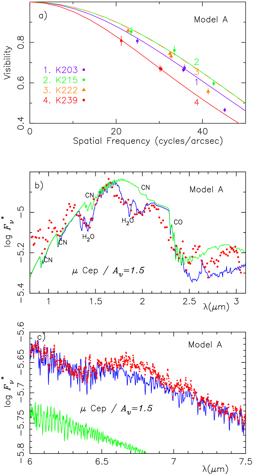
Figure 2: (a) The predicted band averaged visibilities (solid lines) based on the Model A for molsphere + photosphere ($T_{\rm eff}=3600$ K, $T_{\rm ex}=1500$ K, $R_{\rm in}\approx 2.0\,R_{*}$, $N_{\rm col}$(H₂O) = $N_{\rm col}$(CO) = $3.0\times 10^{20}$ cm^-2) are compared with the observed results for $\mu$ Cep (filled symbols) in the 4 narrow bands by Perrin et al. (2005). (b) The predicted near infrared spectrum based on the Model A is compared with the spectrum of $\mu$ Cep observed with the Stratoscope (resolution $R\approx 200$) and corrected for the interstellar reddening with $A_{v}=1.5$ mag. The predicted spectrum of the photosphere, which shows only CN and CO bands but not H₂O, is also shown. (c) The predicted spectrum based on the Model A is compared with the spectrum of $\mu$ Cep observed with the ISO SWS (resolution $R\approx 1600$) and corrected for the interstellar reddening with $A_{v}=1.5$ mag. The predicted spectrum of the photosphere appears at the lower left corner.

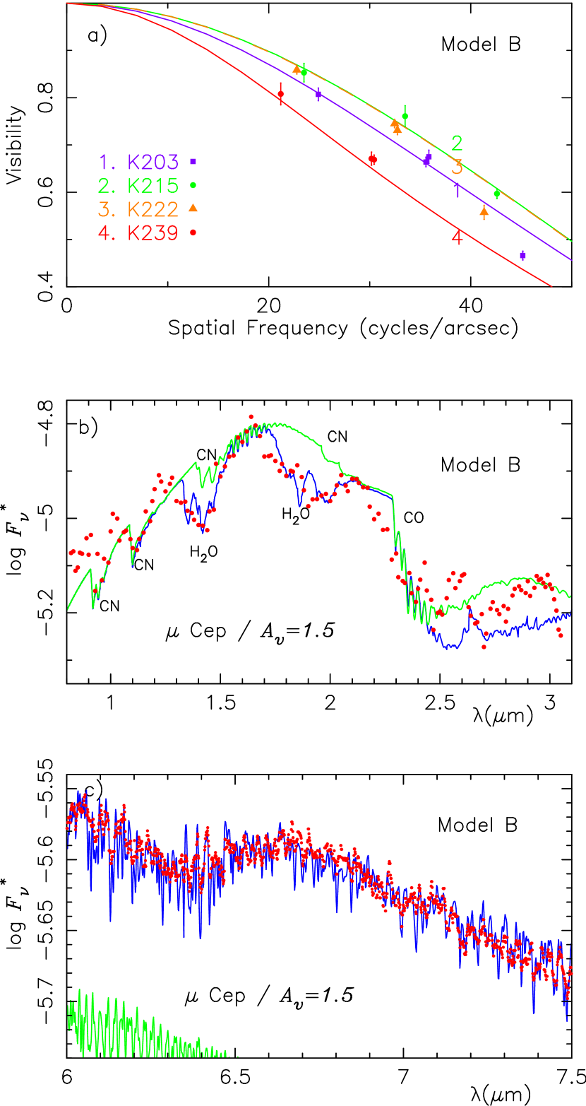
Figure 3: (a) The same as Fig.2a, but for the Model B ($T_{\rm eff}=3800$ K, $T_{\rm ex}=1500$ K, $R_{\rm in}\approx 2.2\,R_{*}$, $N_{\rm col}$(H₂O) = $N_{\rm col}$(CO) = $3.0\times 10^{20}$ cm^-2). (b) The same as Fig.2b, but for the Model B. (c) The same as Fig.2c, but for the Model B.

As a boundary condition to the outer atmosphere, we use the classical spherically extended LTE model photospheres in radiative and hydrostatic equilibrium. The basic parameters we have applied are summarized in Table 1. We keep most of the basic parameters of the photosphere we have used before (Tsuji 2000a,b). It is true that even the effective temperatures of red supergiants are not yet well established, and there is no definitive answer at present. We assumed $T_{\rm eff}=3600$,K for $\alpha$ Ori, which is consistent with the recent interferometry determinations (Dyck et al., 1992, 1996, 1998; Perrin et al., 2004a). We changed $T_{\rm eff}$ of $\mu$ Cep to be 3800,K by the reason to be discussed in Sect.3.2. The effect of $T_{\rm eff}$ on the predicted infrared spectra can be seen by comparing Fig.2b and Fig.3b, for example.

The CNO abundances are most important, since they give direct effect on the infrared spectra. We reanalyzed the equivalent width data of OH and NH measured on the FTS spectra of Betelgeuse by Lambert et al. (1984) with our model photosphere of $T_{\rm eff}=3600$ K, and we confirmed the N and O abundances for the case of $T_{\rm eff}=3600$ K determined by Lambert et al. (1984), who analyzed the effect of $T_{\rm eff}$ on the derived CNO abundances. As for the C abundance, we analyzed some weak lines of the CO first overtone bands measured from the high resolution FTS spectra and our C abundance, as shown in Table 1, is a factor of two smaller than the value of log $A_{\rm C}/A_{\rm H}\approx-3.7$ (for $T_{\rm eff}=3600$ K) by Lambert et al. (1984). The major motivation to have re-analyzed the carbon abundance is the poor fits of the CO features at 1.7 and 2.3 $\mu$m regions in our previous Figs. 2 & 3 (Tsuji 2000a). With our new C abundance, fits in these regions are considerably improved as can be seen in Figs .2b-4b, 7b, and 9a-12a. The micro and macro turbulent velocities are also found from the same analysis and will be discussed elsewhere with details on the abundance analysis (in preparation). The abundance analysis is more difficult for $\mu$ Cep, which shows very broad lines, and we assume the same abundances as for $\alpha$ Ori.

2.2 Model Photospheres

Our model photosphere code is essentially the same as our previous one (Tsuji, 1976), except that the photosphere is now assumed to be spherically symmetric rather than plane-parallel. Also opacity data are updated (see the Appendix of Tsuji (2002a)). We are including the radiation pressure $P_{\rm rad}$ and turbulent pressure $P_{\rm tur}$ in the hydrostatic equilibrium, and thus

$${1\over\rho}{dP_{\rm gas}\over dr}=-g_{\rm eff},$$

where $\rho$ is the density, $P_{\rm gas}$ is the gas pressure, and

$$g_{\rm eff}=g_{\rm grav}-g_{\rm rad}-g_{\rm tur}$$

with

$$g_{\rm grav}=G{M\over r^{2}},$$

$$g_{\rm rad}={4\pi\over c}{\int_{0}^{\infty}\kappa_{\nu}\pi F_{\nu}d\nu},$$

and

$$g_{\rm tur}=-{1\over\rho}{dP_{\rm tur}\over dr}.$$

The notations have their usual meanings, and we assume $P_{\rm tur}=\rho{\xi_{\rm tur}}^{2}$ with the turbulent velocity $\xi_{\rm tur}$. The photosphere is stable so long as $g_{\rm eff}>0$ and this stability limit was defined as the “Eddington limit” for the turbulent plus radiation pressure by De Jager (1984), in analogy with the Eddington’s well known stability limit for the radiation pressure.

Usually, integration of model photosphere starts at a very small optical depth in the continuum (or optical depth in the mean opacity, e.g. Rosseland mean optical depth $\tau_{R}$) such as $\tau_{0}=10^{-6}$. For $T_{\rm eff}=3600$ K and for the other parameters in Table 1, the photosphere extends to $r(\tau_{0}=10^{-6})\approx 730\,R_{\odot}$ with $r(\tau_{0}=1)\approx 650\,R_{\odot}$ as shown by the solid lines in Fig.1. However, it is possible to construct a highly extended model photosphere in radiative and hydrostatic equilibrium, just starting at a still smaller optical depth within the stability limit noted above. An example starting at $\tau_{0}=10^{-14}$ (again $T_{\rm eff}=3600$ K, and other parameters in Table 1) is shown by the dashed lines in Fig.1. The photosphere expands to $r(\tau_{0}=10^{-14})\approx 1700\,R_{\odot}$ for this case, again with $r(\tau_{0}=1)\approx 650\,R_{\odot}$. Thus, within the framework of the classical model photospheres, a model photosphere can be extended, at least formally, to as large as a few stellar radii due to the radiation and turbulent pressures. However, it is to be noted that such a model should not be regarded as physically realistic. In fact, the basic assumption such as LTE should certainly be not applied at such density as low as $10^{-20}$ gr cm^-3 (see Fig.1). For this reason, such a model will not be used in our actual analysis, but only be used as a reference for an ad-hoc model of the molsphere to be discussed in Sect. 2.3.

If we start the integration from a still smaller optical depth or if we assume a somewhat larger turbulent velocity, the photosphere can no longer stay within the De Jager’s generalized Eddington limit and expands without limit. Our purpose here is not to investigate such a stability limit, but we hope that such an extended photosphere may give some clues for medeling the molsphere. Unfortunately, however, the matter included in the extended part (e.g. outside of $\tau_{0}\approx 10^{-6}$) is very small and gives little effect on the spectra as well as on the visibilities. It is difficult to deposit more matter in the upper photosphere within the framework of the hydrostatic equilibrium model, even though a kind of dynamical effect is introduced through the turbulent pressure. One idea may be to consider some kind of shock wave by which the rarefied gas can be compressed and heated (e.g. Woitke et al., 1999), and the extended photosphere will provide the pre-shock condition for such a model.

2.3 Ad hoc Model of the Molspheres

We recognize it difficult to construct a self-consistent model of the molsphere at present, and we use an ad hoc model starting from the extended photosphere discussed in Sect.2.2. We consider a model of molsphere specified with the excitation temperature $T_{\rm ex}$, gas column density $N_{\rm col}$, and inner radius $R_{\rm in}$. Then, in the layers above $r=R_{\rm in}$ in the extended LTE photosphere, the temperatures are replaced with $T_{\rm ex}$ and the matter densities are increase by a factor $N_{\rm col}/N_{\rm LTE}$, where $N_{\rm LTE}$ is the LTE column density of the extended photosphere above $r=R_{\rm in}$. The resulting molsphere is isothermal at $T_{\rm ex}$, with the column density $N_{\rm col}$, and extending between $r=R_{\rm in}$ and the outer radius $r=R_{\rm out}$, which is near that of the starting extended photosphere (e.g. $R_{\rm out}\approx 1700\,R_{\odot}$ if starting from the model of Fig.1). Since the matter density is rather high near the inner radius, the effect of the outer radius is not important, but outer radius can be changed, if necessary, by starting from the extended photospheric model with different $\tau_{0}$ . The matter densities and temperatures below $R_{\rm in}$ conserve the original LTE values of the extended photosphere, but they give little effect on the resulting spectra and visibilities because the matter densities there are very low.

Our model of the molsphere is not a physical model at all, and no longer in radiative and hydrostatic equilibrium, but will be used as a means by which to compute spectra and visibilities, and to infer the physical parameters such as temperature, column density and size of the molsphere from the observed data. This model is essentially the same as just to assume an envelope or shell of given parameters, as is usually done. An advantage of our formulation is that the spectral synthesis and related computer codes being used for the photospheres can directly be used for our molsphere plus photosphere models with almost no changes.

2.4 Spectra and Visibilities

We compute the specific intensity $I_{\nu}(\mu)$ with our spectral synthesis code for 98 values of $\mu$, where $\mu=cos\,\theta$ ($\theta$ is the angle between the normal and the direction to the observer). Then, the flux $F_{\nu}(r)$ is given by:

$$F_{\nu}(r)=2\int_{0}^{1}{\mu I_{\nu}(\mu)d\mu}=2\sum_{i=1}^{98}{w_{i}\mu_{i}I_{\nu}(\mu_{i})}.$$

with the abscissa $\mu_{i}$ and weight factor $w_{i}$ for Gaussian integration . Then, $F_{\nu}^{*}(r)$ corrected for the dilution effect is obtained by

$$F_{\nu}^{*}(r)=r^{2}F_{\nu}(r)/R_{*}^{2},$$

where $R_{*}$ is the stellar radius at $\tau_{R}\approx 1$ and defines the effective temperature $T_{\rm eff}$ through $L_{*}=4\pi R_{*}^{2}\sigma T_{\rm eff}^{4}$ ($L_{*}$ is the stellar luminosity and $\sigma$ is the Stefan-Boltzmann constant).

The spectra are computed with the resolving powers of $5\times 10^{4}$ - $10^{5}$ and convolved with the slit functions matching to the resolutions of the observed spectra. We use the line list including H₂O (Partridge & Schwenke, 1997), OH (Jacquinet-Husson et al., 1999), CO (Guelachivili et al., 1983; Chackerian & Tipping, 1983), SiO (Lavas et al., 1981; Tipping & Chackerian, 1981; Langhoff & Bauschlicher, 1993), and CN(Cerny et al., 1978; Bauschlicher et al., 1988). All these molecular species (H₂O, OH, CO, SiO, CN) are included in the calculation of photospheric spectra, but only H₂O and CO are included in the molsphere.

For a spherically symmetric object with the radius $R$, the visibility $V_{\nu}$ is obtained through the Fourier transform of the strip intensity distribution, $\Phi_{\nu}(x)$, defined by

$$\Phi_{\nu}(x)=2\int_{0}^{\sqrt{(}R^{2}-x^{2})}{I_{\nu}(x,y)dy},$$

where $I_{\nu}(x,y)$ is the intensity at $(x,y)$ on the object surface, and the baseline of the interferometer is in the $x$-direction (Michelson & Pease, 1921). In the numerical analysis of the extended envelope around central star, we follow the formulation we have used before (Tsuji, 1978b): We introduce

$$p={x\over d}/{\theta_{*}\over 2},$$

where $\theta_{*}$ and $d$ are the angular diameter of the central star and distance to the object, respectively, and

$$v={l\over\lambda}/{\theta_{*}\over 2},$$

where $l$ and $\lambda$ are the separation of the two telescopes on the interferometer baseline and wavelength, respectively. Then, the monochromatic visibility $V_{\nu}$ is given by

$$V_{\nu}(v)={\int_{0}^{\infty}{\Phi_{\nu}(p)cos(2{\pi}vp)dp}}/{\int_{0}^{\infty}{\Phi_{\nu}(p)dp}}.$$

For comparison with observed visibilities, which are usually obtained through wide or narrow band filters, the monochromatic visibilities are squared and averaged with the filter transmissions as weights to have the band averaged visibility, following Perrin et al. (2004a).

3 The M Supergiant Star $\mu$ Cephei

With the use of the recent visibility data, we first examine our previous model of the molsphere of $\mu$ Cep based on the infrared spectra alone (Tsuji 2000a,b) and confirm that the model is already reasonably consistent with the recent visibility data (Sect.3.1). We further show that the model can be revised to be more consistent with both the visibility and spectral data (Sect. 3.2). The resulting model, however, does not agree with the model based primarily on the visibility data (Perrin et al., 2005), and we show that the spectral data are as important as the visibility data in modeling the outer atmospheres of cool luminous stars (Sect.3.3).

3.1 Molsphere as Seen by the Infrared Spectra

First, we examine a model based on the parameters derived from the infrared spectra (Tsuji 2000a,b), as summarized in Table 2 under Model A. It is to be remembered that the temperature and column density were estimated from the width and depth of the H₂O 1.9 $\mu$m bands, respectively, on the Stratoscope spectra. The inner radius was estimated from the strength of the H₂O 6.3 $\mu$m bands in emission on the ISO spectrum. Thus, our model consists of the photospheric model of $T_{\rm eff}=3600$ K and the molsphere model characterized by the excitation temperature $T_{\rm ex}=1500$ K, H₂O and CO column densities of $N_{\rm col}\approx 3.0\times 10^{20}$ cm^-2, and inner radius of $R_{\rm in}\approx 1300\,R_{\odot}$ ($\approx 2\,R_{*}$). The molsphere, starting from the extended photosphere of Fig.1, actually extends from $R_{\rm in}\approx 1300\,R_{\odot}$ to $R_{\rm out}\approx 1700\,R_{\odot}$, but effective contribution comes from the layers close to the inner radius where the density is relatively high.

We now examine this model of the photosphere-molsphere with the recent visibility data for the four narrow band regions within the $K$ band by Perrin et al. (2005). We compute the intensity $I_{\nu}(\mu)$ at the spectral resolution of 0.1 cm^-1 for our combined model of the photosphere and molsphere, and the strip intensity distributions and visibilities are evaluated, as outlined in Sect. 2.4. We apply the angular diameter of the central stellar disk of $\theta_{*}=14.11$ mas as estimated by Perrin et al. (2005). In evaluating the band averaged visibility from the monochromatic visibilities, the filter transmission of each narrow band filter is approximated by the Gaussian with the parameters given in Table 1 of Perrin et al. (2004b). In comparing the predicted and observed visibilities, $\chi^{2}$ value is evaluated by

$$\chi^{2}=\sum_{i=1}^{N}\biggl{[}{{V_{i}({\rm obs})^{2}-V_{i}({\rm model})^{2}}\over{\sigma_{i}}}\biggr{]}^{2},$$

where $V_{i}({\rm obs})$ and $V_{i}({\rm model})$ are the observed and prdicted visibilities, respectively, $\sigma_{i}$ is the error estimate to $V_{i}({\rm obs})^{2}$, and $N$ is the data points for each band.

The predicted visibilities based on the Model A are compared with the observed ones by Perrin et al. (2005) in Fig.2a. The fits are pretty good for the $K239$ band which is strongly blanketed with the CO and H₂O lines ($\chi^{2}(K239)=0.23$), and for the $K215$ band relatively free from molecular lines ($\chi^{2}(K215)=5.67$). However, the fits are poor for the $K203$ band which suffers the effect of the H₂O 1.9 $\mu$m bands ($\chi^{2}(K203)=53.68$), and for the $K222$ band which includes no known strong molecular bands ($\chi^{2}(K222)=52.70$). The poor fits in these bands are largely due to the higher predicted visibilities at the highest spatial frequencies compared with the observed ones. Thus, further fine tunings in our modeling should be required.

The predicted near infrared spectrum based on the Model A is compared with the Stratoscope spectrum in Fig.2b. In the following comparisons of the observed and predicted spectra, the observed data are shown by the dots and the predicted spectra by the solid lines in general. The ordinate scale always refers to the predicted spectrum (in unit of the emergent flux from the unit surface area, i.e., in erg cm^-2 sec^-1 Hz^-1), to which the observed one is fitted. Also, the predicted spectrum from the photosphere is shown together with that from the molsphere plus photosphere in most cases. The details of the Stratoscope spectra and the ISO spectra were discussed before (Tsuji, 2000a, b), and all the spectra of $\mu$ Cep are dereddened with $A_{V}=1.5$ mag.

This comparison of the Stratoscope spectra with the predicted ones has already been done before (Tsuji, 2000a), but some improvements are done since then. First, the extra molecular layer was approximated by a plane parallel slab in the previous analysis, and this was thought to be a reasonable approximation for the near infrared. However, the result based on the spherical molsphere shown in Fig.2b reveals that the sphericity effect is already important in the near infrared. This is clearly seen in the CO first overtone bands around 2.5 $\mu$m, whose excess absorption was too large in the previous analysis (see Fig.3 of Tsuji (2000a)) compared with the present result in Fig.2b. This is because the emission in the extended molsphere already has significant contribution to the integrated spectrum. The predicted CO absorption around 2.5 $\mu$m, however, still appears to be deeper compared with the observed. So far, we assumed that the column density estimated from the H₂O features applies to CO as well, but it may be possible that the CO column density is somewhat smaller. But we assume that the column densities for CO and H₂O are the same for simplicity.

Second, the region of the CO second overtone bands around 1.7 $\mu$m, which was depressed too much compared with the observation in our previous analysis (Fig.3 of Tsuji (2000a)), is now improved in Fig.2b, and this is the effect of the revised carbon abundance noted in Sect.2.1. Also, the improved fit near 2.5 $\mu$m is partly due to the revision of the carbon abundance as well. As a result, the near infrared spectrum observed by Stratoscope including the H₂O 1.4 and 1.9 $\mu$m bands can be well matched with our prediction based on the Model A. Although the observed flux short-ward of 1.3 $\mu$m shows some excess compared to the prediction, this may be a problem of the photospheric spectrum, which is also shown in Fig.2b and shows only CO and CN bands.

The predicted spectrum in the H₂O $\nu_{2}$ band region based on the Model A is compared with the ISO spectrum in Fig.2c. This comparison has also been done before with the use of the spherically extended molsphere model (Tsuji, 2000b), but we now use the H₂O line list by Partridge & Schwenke (1997) instead of the HITEMP database (Rothman, 1997) used before. The tendency that the H₂O $\nu_{2}$ bands appear in emission can be well reproduced with our Model A, but the predicted emission is still not strong enough to explain the observed spectrum in the region around 6.8 $\mu$m. The predicted spectrum based on the model photosphere appears at the lower left and the most lines seen are due to the tail of the CO fundamental bands.

3.2 Some Fine Tunings and a Resulting Model

Inspection of Figs. 2a-c reveals that the predicted visibilities and near infrared spectra based on the Model A are not yet fully consistent with the observations. The major problem is that the predicted visibilities at the $K203$, especially at the highest spatial frequency, are much higher than the observed. Also, the predicted emission of the H₂O $\nu_{2}$ bands is not sufficiently strong to be consistent with the observation. Such inconsistencies can be relaxed by changing (a) the excitation temperature of the molsphere, (b) the inner radius, and/or (c) the gas column density. However, the column density is already well consistent with the near infrared spectrum and we will not consider the possibility (c) further. Also, since the visibilities based on the model A are already well consistent with the observations at $K215$ and $K239$ bands, the possibilities (a) and (b) must be considered so that the good fits in the visibilities already achieved can be conserved. We examine the possibilities (a) and (b) systematically by changing the temperature by a step of 100K and the inner radius by a step of 0.1$\,R_{*}$. Also, as to the observed excess in the short-ward of 1.3 $\mu$m, we notice that the recent angular diameter measurements suggested a higher effective temperature of 3789K (Perrin et al., 2005), and we apply $T_{\rm eff}=3800$ K in all the models to be discussed below, instead of 3600 K used in the Model A. The extended phtosphere of $T_{\rm eff}=3800$ K, used as the starting model for the molsphere, is quite similar to the case of $T_{\rm eff}=3600$ K shown in Fig.1.

First, we examine the effect of changing $R_{\rm in}$ from 2.0 $R_{*}\approx 1300\,R_{\odot}$ of the Model A, keeping $T_{\rm ex}$ to be 1500 K. After some trials and errors, we find that a case of $R_{\rm in}\approx 2.2\,R_{*}\approx 1430\,R_{\odot}$ shows some improvements. First, the resulting predicted visibilities for the four narrow band regions are compared with the observed data in Fig.3a: The fits for the $K203$ and $K222$ bands are somewhat improved with $\chi^{2}(K203)=40.51$ and $\chi^{2}(K222)=40.95$, but still not very good. On the other hand, fits for the $K215$ and $K239$ bands remain reasonable with $\chi^{2}(K215)=4.66$ and $\chi^{2}(K239)=13.61$. The good fits in the visibilities for the $K239$ band with the Model A is somewhat degraded but still remain to be reasonable. Second, the predicted flux in the region short-ward of 1.3 $\mu$m is increased as a result of changing $T_{\rm eff}$ of the photosphere to 3800K from 3600K, and the fit in this region now appears to be reasonable as shown in Fig.3b. Finally, the observed and predicted spectra in the 6 - 7 $\mu$m region are compared in Fig.3c. The predicted emission around 6.8 $\mu$m increases appreciably and it is now sufficiently large to account for the observed emission as shown in Fig.3c. We refer to this model as Model B and its major parameters are summarized in Table 2.

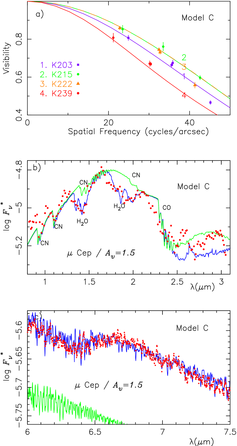
Figure 4: (a) The same as Fig.2a, but for the Model C ($T_{\rm eff}=3800$ K $T_{\rm ex}=1600$ K, $R_{\rm in}\approx 2.0\,R_{*}$, $N_{\rm col}$(H₂O) =$N_{\rm col}$(CO) = $3.0\times 10^{20}$ cm^-2). (b) The same as Fig.2b, but for the Model C. (c) The same as Fig.2c, but for the Model C.

Although the model B is considerably improved compared to the model A, we examine another possibility of changing $T_{\rm ex}$ of the molsphere from 1500 K of Model A while $R_{\rm in}$ remains to be 2.0 $R_{*}$. The resulting predicted visibilities for a case of $T_{\rm ex}=1600$ K are again compared with the observed ones in Fig.4a: The fits for the $K203$ and $K222$ bands are both improved compared to the results for the model B, with $\chi^{2}(K203)=29.24$ and $\chi^{2}(K222)=27.76$. At the same time, fits for the $K239$ band is further degraded but still remain to be acceptable with $\chi^{2}(K239)=17.68$. The fits for the $K215$ band remain fine with $\chi^{2}(K215)=4.52$, and this result that the fits for the $K215$ band remain nearly unchanged may be a natural consequence that this band region is a good continuum window. We conclude that this model, to be referred to as Model C, provides better fits to the observed visibilities compared to the Model B. The predicted near infrared spectrum shown in Fig.4b shows almost no change from Fig.3b, and we confirm that the 1.4 and 1.9 $\mu$m absorption bands depend primarily on the column density which is unchanged throughout. The predicted emission around 6.8 $\mu$m reasonably account for the observed emission as shown in Fig.4c. The major parameters of the Model C are summarized in Table 2.

We examined several other models around the models B and C, but no significant improvements were obtained. For example, a case of increasing $R_{\rm in}$ to 2.1 $R_{*}$, keeping $T_{\rm ex}=1600$ K, results in degrading the fits in visibilities, although fits in spectra remain nearly the same. A case of increasing $T_{\rm ex}$ to 1700 K, keeping $R_{\rm in}=2.0\,R_{*}$, also results in degrading the fits in visibilities, while fits in spectra remain nearly the same. If $R_{\rm in}$ is decreased to $1.9\,R_{*}$ at $T_{\rm ex}=1700$ K, the fits in visibilities for the $K222$ band are somewhat improved compared to those for the Model C, but the predicted emission around 6.8 $\mu$m is reduced to the level of the Model A. On the other hand, if $T_{\rm ex}$ is decrease to 1400 K, $R_{\rm in}$ had to be increased to $2.2\,R_{*}$ to keep the reasonable fits for the spectra, but the fits for the visivilities are degraded appreciably.

We conclude that the Model C is a possible best model that reasonably accounts for both the observed visibilities and infrared spectra simultaneously, within the framework of our highly simplified molsphere model. It is encouraging that our model could reproduce the general tendency that the visibilities in the region with strong H₂O and/or CO bands ($K203,K239$) are lower than those in the region with less molecular absorption ($K215,K222$), in agreement with the observations, even though the fits are not very good for the $K203$ and $K222$ bands. This result implies that the molsphere model based on the infrared spectra alone is reasonably consistent with the visibility data not known at the time when the modeling was done. This may be because the infrared spectra already include some information on the spatial structure of the extended atmosphere. It is most important, however, that the model is now examined directly with the interferometry, which is a direct probe of the spatial structure of the astronomical objects.

3.3 Molsphere as seen by the Visibility Data

We notice, however, that the model parameters of our Model C show significant differences with those derived from the visibility data by Perrin et al. (2005) themselves: Their excitation temperature is near 2700 K compared with 1600 K of our Model C and their radius of the molecular layer is about 1.3 $R_{*}$ compared with the inner radius 2.0 $R_{*}$ of our Model C. To investigate the origin of the differences, we think it useful to analyze their model in the same way as in our models. For this purpose, we refer to a model based on their parameters as Model D. Since their molecular layer is assumed to be a thin shell, we design the Model D in our formulation to be extending from $R_{\rm in}=851\,R_{*}$ to $R_{\rm out}=858\,R_{*}$, for which the initial extended photosphere starts at $\tau_{0}=10^{-8}$, and thus the effective location of the thin shell of the Model D is at about $r\approx 1.3\,R_{*}$.

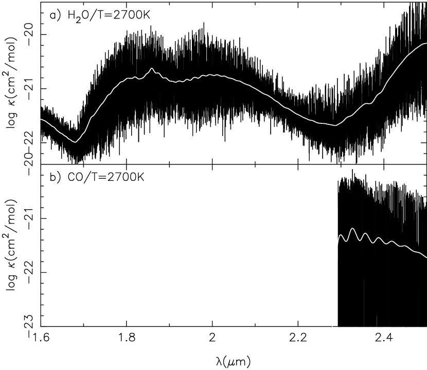
Figure 5: a) Absorption cross-section (cm² molecule^-1) of H₂O at $T=2700$K. The black line is by the high resolution ($R\approx 50000$) and the white line is the straight mean opacity smeared out with the resolution $R\approx 1600$. b) The same as for a) but for CO.

The gas column densities were not provided in the model of Perrin et al. (2005) but a mean optical thickness for each narrow band region was given. Accordingly, we transform their optical thickness at each filter band region to the column densities with the absorption cross sections of CO and H₂O evaluated from the line list mentioned in Sect.2.4 and shown in Fig.5, where the high resolution results are given with the black while the smeared out straight means by the white lines. The resulting column densities summarized in Table 3 appear to be different for different bands, while this should be the same at least for 2.03, 2.15 and 2.22 $\mu$m in which H₂O is the major source of opacity. The column density of CO can of course be different from that of H₂O. We assume that the column densities of CO and H₂O for the 2.39 $\mu$m region are the same as in Table 3, just as an example. But the optical thickness of 3.93 for the 2.39 $\mu$m region given by Perrin et al. (2005) is large enough to completely mask the photospheric spectra and the column density corresponding to $\tau=3.93$ should anyhow be very large.

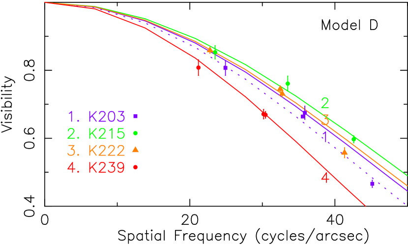
Figure 6: The predicted band averaged visibilities based on the monochromatic visibilities are shown by the solid lines for the Model D ($T_{\rm eff}=3800$ K, $T_{\rm ex}=2700$ K, $R_{\rm in}\approx 1.3\,R_{*}$, and the optical thickness for the 4 narrow band regions given in Table 3). It is confirmed that the results for the $K215,K222$, and $K239$ bands based on the column densities estimated with the cross-sections of the contributing molecular bands (Fig.5) reproduce the predicted visibilities based on the mean optical thicknesses (Fig.1 of Perrin et al.(2005)). The results also agree with the observed visibilities for $\mu$ Cep by Perrin et al (2005) shown by the filled symbols. But the result for the $K203$ band for log $N_{\rm col}=1.4\times 10^{20}$ cm^-2 in Table 3 (solid line labelled with 1) does not reproduce the result of Perrin et al.(2005). Instead we find that reasonable agreements with the predicted as well as observed values by Perrin et al.(2005) can be obtained for log $N_{\rm col}=4.2\times 10^{20}$  cm^-2 (dotted line).

The major parameters of the Model D are summarized in Table 2 and we can now proceed as in our Models A - C with these parameters. The resulting visibilities are shown in Fig.6 together with the observed data by Perrin et al. (2005). The predicted visibilities using the column densities as input parameters nearly reproduce the ones for the $K215,K222$, and $K239$ bands shown in Fig.1 of Perrin et al. (2005) using the effective optical thicknesses as input parameters. However, such an agreement cannot be found for the $K203$ band, and this means that the transformation of the mean optical depth to the column density could not be done correctly. We cannot understand the reason for this, but the H₂O cross-section at temperature as high as 2700 K may not necessarily be accurate enough for the region of the $K203$ band. Thus, we may conclude that the visibility computed with the mean optical thickness can be a reasonable approximation to the one based on the monochromatic visibilities evaluated with the realistic line list at high spectral resolution, only if the optical thickness correctly reflects the detailed line opacities. .

As shown in Fig.6, the predicted visibilities based on the Model D show fine fits with the observed ones for the $K215,K222$, and $K239$ bands, for which $\chi^{2}(K215)=4.02$, $\chi^{2}(K222)=14.23$, and $\chi^{2}(K239)=2.32$. This is what can be expected, since our visibilities agree well with those by Perrin et al. (2005), which are already known to be well consistent with the observed data. For the same reason, the fits for the $K203$ band are quite poor with $\chi^{2}(K203)=47.93$. It is, however, possible to improve the fits in the $K203$ band by just changing the column density somewhat, and we find a reasonable fit with $\chi^{2}(K203)=16.99$ for $N_{\rm col}$(H₂O)$=4.2\times 10^{20}$ cm^-2 after a few trials and errors (see dotted line in Fig. 6). If we can choose four values for the free parameter such as the mean optical depth or the column density for the four observed data, it is certainly possible to have good fits for all the observed data. However, such fits cannot be regarded as justification of such a model as D, since the values of the column densities are so different for the different bands (see Table 3).

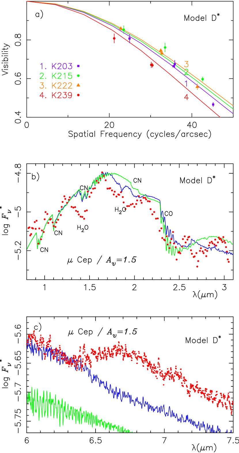
Figure 7: (a) The same as Fig.2a, but for the Model D^∗ ($T_{\rm eff}=3800$ K, $T_{\rm ex}=2700$ K, $R_{\rm in}\approx 1.3\,R_{*}$, $N_{\rm col}$(H₂O) = $2.8\times 10^{20}$ cm^-2, $N_{\rm col}$(CO) = $9.3\times 10^{21}$ cm^-2). (b) The same as Fig.2b, but for the Model D^∗. (c) The same as Fig.2c, but for the Model D^∗.

Since the column densities should be unique for the different bands, we modify the Model D so that $N_{\rm col}$(H₂O)$=2.8\times 10^{20}$ cm^-2, just as an example, for all the 4 narrow band regions. Then, to account for $\tau=3.93$ of the $K239$ band which includes CO and H₂O, it turns out that $N_{\rm col}$(CO)$=9.3\times 10^{21}$ cm^-2 with the absorption cross-sections given in Table 3. For this modified Model D, to be referred to as Model D^∗, we first evaluate the visibilities and the results are again compared with the observed data in Fig.7a. The fits are generally fair with $\chi^{2}(K203)=17.78$, $\chi^{2}(K215)=25.24$, $\chi^{2}(K222)=14.21$, and $\chi^{2}(K239)=30.45$. The fits for the $K203$ and $K222$ bands are better than those for the Model C while the fits for the $K215$ and $K239$ bands are better in the Model C. Thus, it is difficult to decide which of the Model C or Model D^∗ is to be preferred from the visibility analysis alone.

An advantage of using the column density instead of the mean optical thickness is that the spectra can be evaluated for the same input parameters. The near infrared spectrum for the Model D^∗ is compared with the Stratoscope data in Fig.7b. The fit is rather poor and the other $N_{\rm col}$(H₂O) values in Table 3 produce too weak or too strong H₂O absorption bands. We also evaluate the spectrum in the 6 - 7 $\mu$m region for $N_{\rm col}$(H₂O)$=2.8\times 10^{20}$ cm^-2 and compared with the ISO data in Fig.7c. The predicted spectrum still appears in absorption and cannot be matched with the observed one at all. The results are more or less the same for other values of $N_{\rm col}$(H₂O) in Table 3.

In our fine tunings in Sect.3.2, we increased the temperature from 1600 to 1700 K and, at the same time, decreased the inner radius to from 2.0 to 1.9 $R_{*}$, and obtained reasonable fits to the observed visibilities. If we pursued a solution in this direction, we might increase the temperature further and decrease the inner radius at the same time. The resulting model might be similar to the Model D^∗, but we might reject such a case since such a high temperature - small size model might not explain the 6 - 7 $\mu$m emission as can be inferred from the result shown in Fig.7c. Perrin et al. (2005) did not consider the spectral data and might be led to the high temperature - small size model that might have satisfied the visibility data well.

We conclude that it is difficult to decide the unique solution for the molsphere model from the visibility data alone, and it is indispensable to apply the spectroscopic data at the same time to have some idea on the model of the stellar outer atmosphere. At the same time, it is difficult to have good fits to the observed visibilities at all the spatial frequencies within the framework of the simplified uniform spherically symmetric models of the molsphere. Certainly, some details of the fine structure of the outer envelope should be considered to have better fits at higher spatial frequencies, and our present analysis is only a very initial stage on the interpretation of the visibility data.

4 The Case of $\alpha$ Orionis

Betelgeuse is an object probably best observed with a variety of methods and new observed data are still accumulating. At the same time, Betelgeuse is a quite complicated object, and how to interpret the observed data is still controversial at least partly. We will show that unexpected water lines observed in Betelgeuse may be difficult to be explained by anomalies within the framework of the photospheric models (Sect. 4.1). On the other hand, the infrared spectra and visibility data consistently show the presence of the extra molecular layers and provide consistent estimations of their basic parameters (Sect. 4.2). In the mid infrared region, some recent observations subjected to controversy, but we look for a possibility to relax such an issue (Sect .4.3).

4.1 Can a Cool Photosphere Explain the Infrared Spectra of Betelgeuse?

This is a question addressed recently by Ryde et al. (2006), who observed high resolution spectra of Betelgeuse in the 12 $\mu$m region and suggested that the observed H₂O lines can be interpreted with the anomalous structure of the photosphere rather than assuming the presence of the extra molecular layers. They showed that their high resolution 12 $\mu$m spectra could be well fitted with the predicted ones based on the cool photospheric models. However, it can be shown below that the near infrared spectra cannot easily be matched by an anomalous structure of the photosphere.

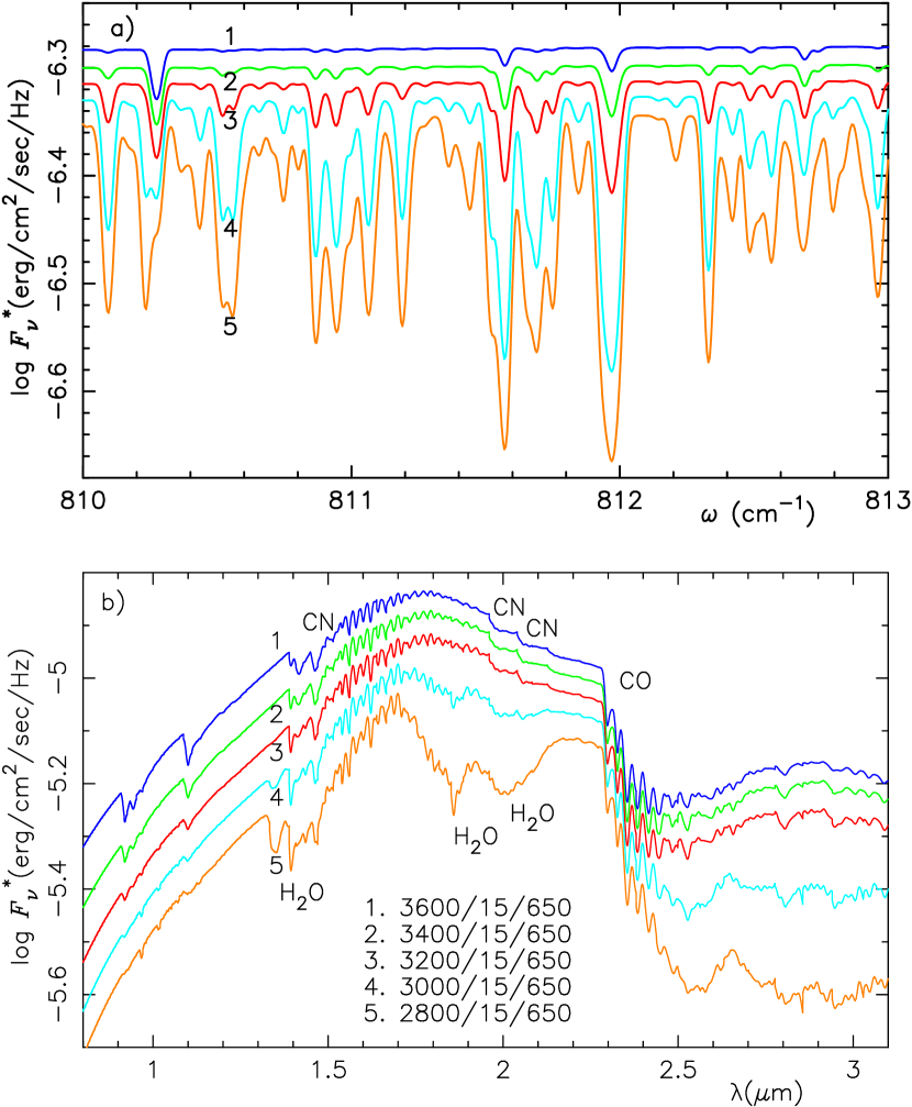
Figure 8: (a) Predicted spectra of water in the 12 $\mu$m region (spectral resolution of 0.005 cm^-1 and broadened with the macro-turbulence of 10 km s^-1) based on the LTE classical model photospheres with the parameters in Table 1 except for $T_{\rm eff}$’s, which are 1: 3600 K, 2: 3400 K, 3: 3200 K, 4: 3000 K, and 5: 2800 K. Some lines of water can be seen already at $T_{\rm eff}\approx 3600$ K and stronger in the cooler models. (b) The same as (a), but for the near infrared region (spectral resolution of 0.1 cm^-1 and convolved with the slit function of FWHM = 1500  km s^-1). Since the $f$-values of H₂O lines are about 1 - 2 orders of magnitude smaller in this region compared with those in the the 12 $\mu$m region, water bands can be seen only in the models with $T_{\rm eff}\lesssim 3000$ K.

Ryde et al. (2006) suggested that the observed H₂O pure rotational lines in Betelgeuse can be accounted for with the thermal structure approximated by the classical model photosphere of $T_{\rm eff}\approx 3250$ K and that their observations can be explained with a rather small H₂O column density of $N_{\rm col}\approx 5\times 10^{18}$ cm^-2. This is possible because the $f$-values of the H₂O pure rotational lines are pretty large. In Fig.8a, the spectra of the H₂O pure rotation lines predicted from the classical spherically extended model photospheres of $T_{\rm eff}$ = 2800, 3000, 3200, 3400, and 3600 K ($M=15\,M_{\odot}$, $R=650\,R_{\odot}$, $\xi_{\rm micro}=5$ km s^-1, $\xi_{\rm macro}=10$ km s^-1, throughout) are shown. Thus, weak H₂O pure rotational lines can be observed already at $T_{\rm eff}$ = 3600 K and increasingly stronger towards the lower $T_{\rm eff}$ ’s. At $T_{\rm eff}\approx 3200$ K, H₂O lines can certainly be observed even if they are diluted by the silicate dust emission in Betelgeuse.

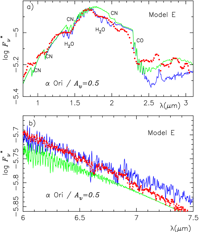
Figure 9: (a) The predicted near infrared spectrum based on the Model E ($T_{\rm ex}=1500$ K, $R_{\rm in}\approx 1.7\,R_{*}$, $N_{\rm col}$ = $1.0\times 10^{20}$ cm^-2) is compared with the spectrum of $\alpha$ Ori observed with Stratoscope (resolution $R\approx 200$) and corrected for the interstellar reddening with $A_{v}=0.5$ mag. The predicted spectrum of the photosphere is also shown. (b) The predicted spectrum of the H₂O $\nu_{2}$ band region based on the Model E is compared with the spectrum of $\alpha$ Ori observed with the ISO SWS (resolution $R\approx 1600$) and corrected for the interstellar reddening with $A_{v}=0.5$ mag. The predicted spectrum of the photosphere appears below that for molsphere + photosphere.

However, with such a small column density, it is not possible to explain the H₂O 1.4 and 1.9 $\mu$m bands observed with Stratoscope II, since the $f$-values of the near infrared H₂O lines are 1 - 2 orders of magnitude smaller than those of the pure-rotation lines observed in the 12 $\mu$m region. In Fig.8b, we show the near infrared spectra predicted from the same models as used for Fig.8a and reduced to the resolution of the Stratoscope observations. It can be confirmed that the H₂O 1.4 and 1.9 $\mu$m bands cannot be seen in the models with $T_{\rm eff}=3200$ K and higher, but appear in the models of $T_{\rm eff}=3000$ K and lower. It is clear that the H₂O 1.4 and 1.9 $\mu$m bands seen on the Stratoscope spectra (Figs.9a - 12a) cannot be accounted for with the cool photosphere of $T_{\rm eff}\approx 3250$ K. Ryde et al. (2006) argued that the photosphere of Betelgeuse can be very peculiar, but the relative behaviors of the near and mid infrared spectra should remain nearly the same so long as any peculiarity remains within the photosphere. We conclude that the near and mid infrared spectra cannot be consistently interpreted by a cool atmosphere wihin the framework of the classical model photosphere. On the other hand, Ryde et al. (2006) suggested a possibility of an inhomogeneous atmosphere with a cool component giving rise to the 12 $\mu$m water lines and a hot component giving rise to the near-infrared H₂O bands. Such a possibility should hopefully be examined further with other arguments suggesting the inhomogeneity in red supergiant stars (Sect. 5.1).

4.2 Can a Molsphere Explain the Infrared Spectra of Betelgeuse?

For Betelgeuse, we have assumed the presence of an extra molecular layer above the photosphere, and estimated $T_{\rm ex}=1500\pm 500$ K and $N_{\rm col}=10^{20}$ cm^-2 from the Stratoscope spectra based on a simple slab model (Tsuji, 2000a). Also, we have suggested that the weak 6.6 $\mu$m absorption observed with ISO can be explained if the inner radius of the molsphere is $R_{\rm in}\approx 1.5R_{*}$ (Tsuji, 2000b). This result, however, was given without a detailed numerical analysis and may not be accurate enough. We now re-examine such a model of Betelgeuse in some detail with some improvements such as noted in the analysis of $\mu$ Cep. The observed spectra of Betelgeuse are discussed in detail before (Tsuji, 2000a, b) and dereddened with $A_{\rm V}=0.5$ mag.

For this purpose, we recall that the near infrared spectra observed with Stratoscope II are relatively free from the effect of spherical extension of the molsphere, and thus they are very useful probes of the column density and temperature. Especially, we believe that the column density of H₂O can be well fixed from the strengths of the 1.4 and 1.9 $\mu$m bands to be $N_{\rm col}\approx 10^{20}$ cm^-2. We confirm that this result remains unchanged for possible values of $T_{\rm ex}$ and $R_{\rm in}$ in the spherically extended molsphere models. Then, although the H₂O 6.3 $\mu$m bands do not appear in emission but only in weak absorption in the case of $\alpha$ Ori, they can be used to constrain the extension of molsphere and to refine the temperature. Thus the nature of the extra molecular layer can also be inferred from these infrared spectra alone as in the case of $\mu$ Cep. The result should further be examined in the light of the interferometric observations. For this purpose, we refer to the recent work by Perrin et al. (2004a), who suggested a 2055 K layer located at 0.33 $R_{*}$ above the photosphere from the visibility data at the $K,L,$ and 11.15 $\mu$ bands.

We assume $T_{\rm eff}=3600$ K for the central star and start from the extended photosphere of Fig.1. We examine first the case of $T_{\rm ex}=1500$ K and systematically changed the inner radius $R_{\rm in}$ of the molsphere from 1.3 $R_{*}$, approximately the radius of the molecular layer by Perrin et al. (2004a). The near infrared spectrum can be fitted reasonably well for any values of $R_{\rm in}$ up to $\approx 2\,R_{*}$ with $N_{\rm col}=10^{20}$ cm^-2, but the 6 - 7 $\mu$m spectrum appears in strong absorption for $R_{\rm in}\approx 1.3\,R_{*}$ and weakens towards larger $R_{\rm in}$. It finally turns to emission for $R_{\rm in}\approx 1.9\,R_{*}$. After all, reasonable fits in the 6 - 7 $\mu$m region as well as in the near infrared spectra can be obtained for $R_{\rm in}\approx 1.7\,R_{*}$ (Model E) as shown in Fig.9. However, the predicted spectrum shows appreciable excess in the region long-ward of 7 $\mu$m compared with the ISO spectrum as shown in Fig.9b.

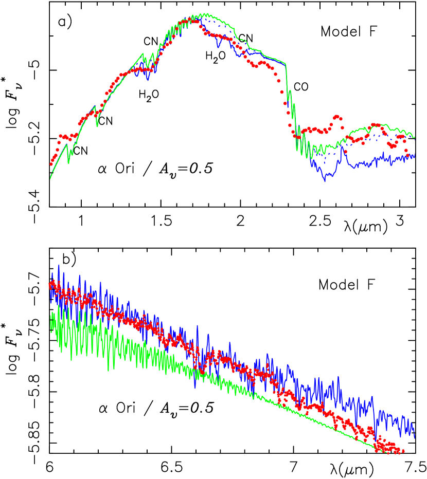
Figure 10: (a) The same as Fig.9a, but for the Model F ($T_{\rm ex}=1750$ K, $R_{\rm in}\approx 1.5\,R_{*}$, $N_{\rm col}$ = $1.0\times 10^{20}$ cm^-2). The dotted line is for the case of $N_{\rm col}$ = $2.0\times 10^{19}$ cm^-2 suggested by Verhoelst (2006). (b) The same as Fig.9b, but for the Model F.

Next, we examine the case of $T_{\rm ex}=1750\,$K, and reasonable fits in the near infrared and 6 - 7 $\mu$m regions are obtained for $R_{\rm in}\approx 1.5\,R_{*}$ (Model F) as shown in Figs.10a and b, respectively. This case is close to the Verhoelst et al. (2006)’s model except for the column density. We examined their value of $N_{\rm col}=2\times 10^{19}$ cm^-2 and the resulting near IR spectrum is shown by the dotted line in Fig.10a. This column density may be too small to explain the H₂O 1.4 and 1.9 $\mu$m bands. The dip at 6.6 $\mu$m due to the H₂O $\nu_{2}$ bands can be reasonably accounted for but the disagreement in the region long-ward of 7 $\mu$m cannot be resolved as shown in Fig.10b.

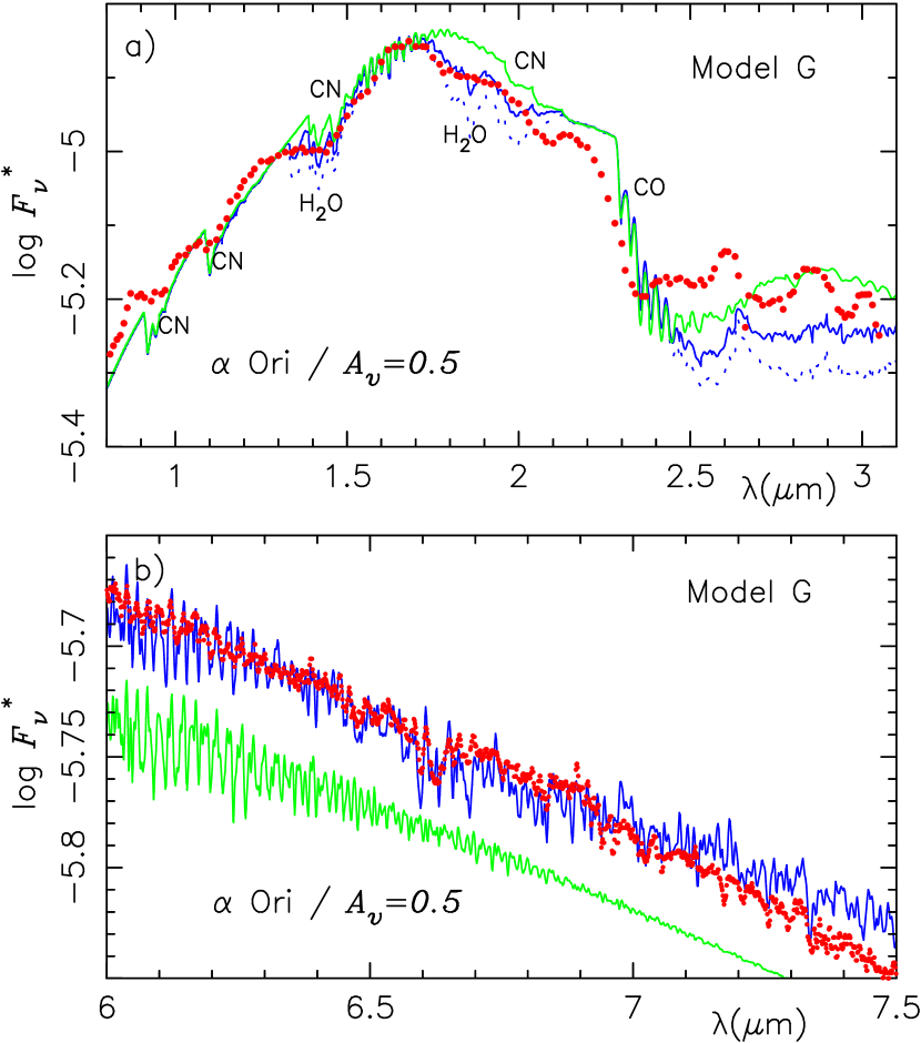
Figure 11: (a) The same as Fig.9a, but for the Model G ($T_{\rm ex}=2000$ K, $R_{\rm in}\approx 1.4\,R_{*}$, $N_{\rm col}$ = $1.0\times 10^{20}$ cm^-2). The dotted line is for the case of $N_{\rm col}$ = $2.0\times 10^{20}$ cm^-2 suggested by Ohnaka (2004). (b) The same as Fig.9b, but for the Model G.

For the case of $T_{\rm ex}=2000\,$K, a possible best fits are obtained for $R_{\rm in}\approx 1.4\,R_{*}$ (Model G) as shown in Fig.11. This case is close to the Ohnaka (2004)’s model except for the column density, and we examined his value of $N_{\rm col}=2\times 10^{20}$ cm^-2. The resulting near IR spectrum is shown by the dotted line in Fig.11a, and this column density may be too large to account for the H₂O 1.4 and 1.9 $\mu$m bands. The near infrared spectrum is relatively insensitive to $T_{\rm ex}$ and $R_{\rm in}$, but depends critically on $N_{\rm col}$. The predicted excess in the region long-ward of 7 $\mu$m compared with the ISO spectrum is somewhat relaxed but the excess still remains as shown in Fig.11b.

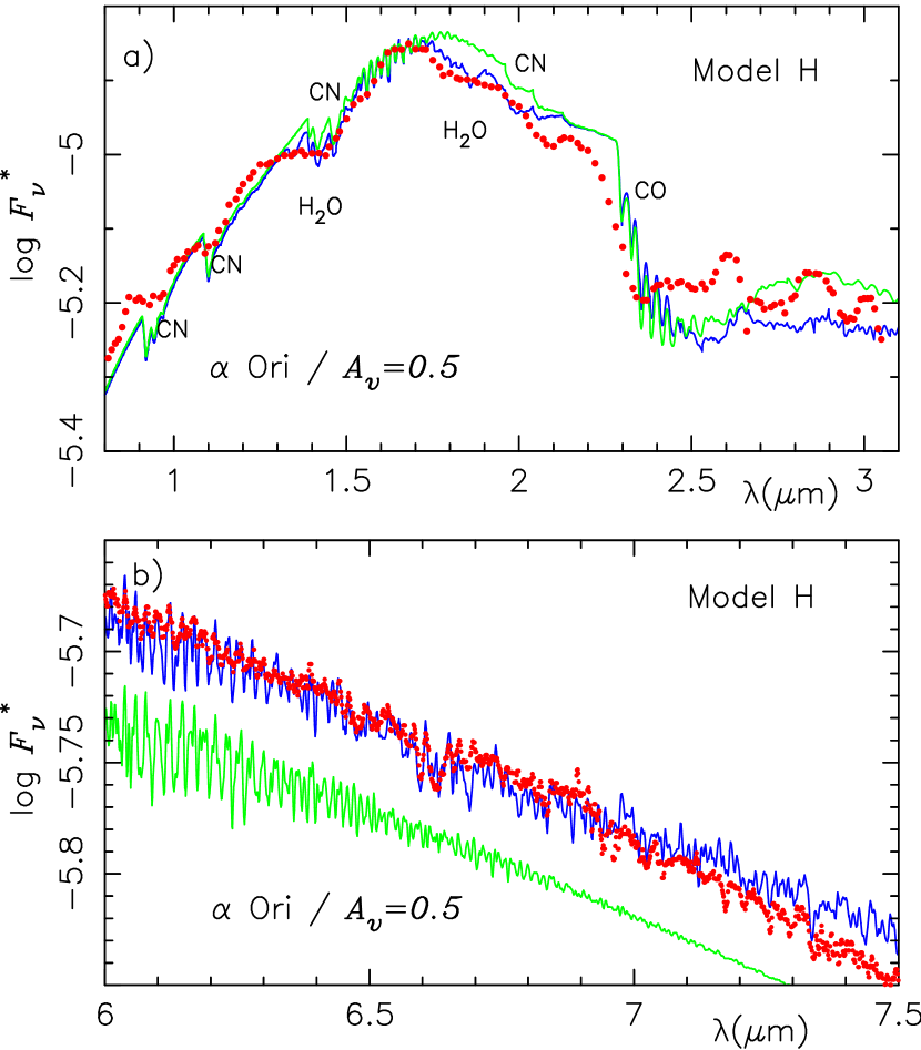
Figure 12: (a) The same as Fig.9a, but for the Model H ($T_{\rm ex}=2250$ K, $R_{\rm in}\approx 1.3\,R_{*}$, $N_{\rm col}$ = $1.0\times 10^{20}$  cm^-2). (b) The same as Fig.9b, but for the Model H.

With a hope to improve the fits further, we examined the case of $T_{\rm ex}=2250\,$K. In this case, $R_{\rm in}\approx 1.3\,R_{*}$ (Model H) results in reasonable fits as shown in Fig.12. Although the fits do not show any drastic improvements, inspection of the cases of $T_{\rm ex}$ from 1500 K to 2250 K reveals that the fits in some details (e.g. strengths of the absorption features, overall shape of the spectra etc.) are generally better for the higher $T_{\rm ex}$, as can be seen through Fig.9 to Fig.12. If we further increase $T_{\rm ex}$ to 2500 K, however, absorption and emission in the 6 - 7 $\mu$m region just cancel for $R_{\rm in}\approx 1.3\,R_{*}$. Thus, we may stop our survey here, and we summarize the major parameters of the 4 models discussed above in Table 4.

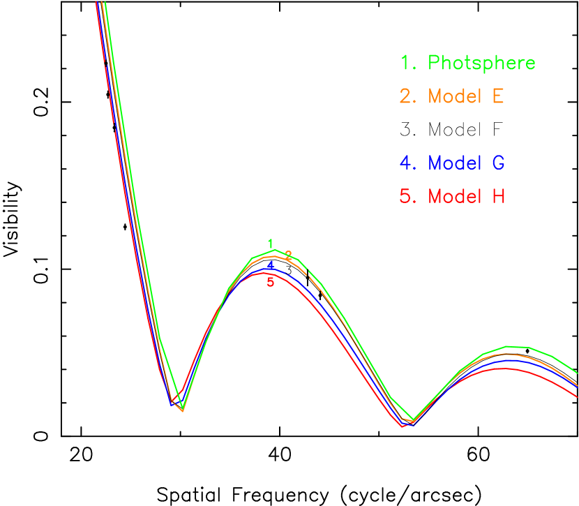
Figure 13: The predicted visibilities for the $K$ band based on the molsphere + photosphere models (Models E- H) (solid lines) are compared with the observed ones in the $K$ bands (filled circles) by Perrin et al. (2004). Also, the predicted band averaged visibility curve (solid line) based on the classical photospheric model ($M=15\,M_{\odot}$, $R_{*}=650\,R_{\odot}$, $T_{\rm eff}=3600$ K, and other parameters in Table 1) is shown for comparison.

For $\alpha$ Orionis, the visibility data at the narrow bands as for $\mu$ Cephei are not yet known, but those at the wide band $K$ filter are available (Perrin et al., 2004a). We evaluate the band averaged visibilities for the standard $K$ band filter as for the narrow band filters discussed in Sect.3, and we assume that the angular diameter of the central stellar disk is $\theta_{*}=42$ mas following Perrin et al. (2004a). First, we compare the visibility curve predicted for the model photosphere of $T_{\rm eff}=3600\,$K ($\tau_{0}=10^{-6}$) with the observed visibility data at the $K$ band in Fig.13, and find that it does not fit well to the observed data ($\chi^{2}=300.99$). The case for the extended photosphere ($\tau_{0}=10^{-14}$) discussed in Sect.2.2 shows only minor changes, and the extended as well as the classical photospheres cannot explain the observed visibilities at the $K$ band.

Next, we compare in Fig. 13 the predicted visibilities at the $K$-band for the 4 models (Models E - H in Table 4) discussed above, and the $\chi^{2}$ values are 134.26, 102.21, 29.56, and 16.18 for the Models E, F, G, and H, respectively. The fits in the first lobe of the visibility curves are better for the models with the higher $T_{\rm ex}$ and smaller $R_{\rm in}$ (i.e. Model G and especially H in Table 4). However, the fits in the second and third lobes appear to be more consistent with the models of the lower $T_{\rm ex}$ and larger $R_{\rm in}$ (i.e. Models E and F in Table 4). The first lobe may reflect the basic structure of the object while the second and third lobes may depend on some fine structures. Thus, considering the consistent results from the infrared spectra and visibilities, we may conclude that the molsphere of Betelgeuse is characterized by the rather compact size ($R_{\rm in}\approx 1.3\,R_{*}$ ), rather high temperature ($T_{\rm ex}\approx 2250\,$K) and modest column density ($N_{\rm col}\approx 10^{20}$ cm^-2) (i.e. the Model H of Table 4). Anyhow, it is clear that the visibility data can be interpreted more consistently with the molsphere around the photosphere. We conclude that a molsphere explains not only the infrared spectra (the mid IR spectra are discussed in Sect. 4.3) but also the $K$ band visibility data consistently.

4.3 What the Mid Infrared Data Tell Us?

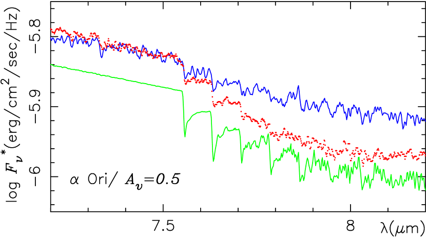
Figure 14: The predicted spectrum around SiO fundamental bands based on the Model H is compared with the spectrum of $\alpha$ Ori observed with the ISO SWS (resolution $R\approx 1600$) and corrected for the interstellar reddening with $A_{v}=0.5$ mag. The predicted spectrum of the photosphere appears below that for the Model H.

The region short-ward of 7.5 $\mu$m discussed in Sect.4.2 may be almost free from the effect of dust, which, however, will have significant effect in the longer wavelength region. First, we examine the SiO feature near 8 $\mu$m, which was used as a further check of the molecular layers by Verhoelst et al. (2006). The band-head region of the SiO fundamentals observed by ISO can be reasonably fitted by our prediction with $N_{\rm col}=10^{20}$ cm^-2 as shown in Fig.14, and this column density may not be high enough to mask the photospheric spectrum. However, the fit in the long-ward of 7.6 $\mu$m is quite poor, and the ISO spectrum shows a large depression centered at about 8 $\mu$m compared with our prediction. This depression may partly be due to the effect of SiO in the molsphere, which we have not considering yet. For simplicity, we have considered only CO and H₂O in the molsphere but the effect of other molecules including SiO should certainly be examined. The effect of dust should still be minor in Fig.14, except for a possible tail of the alumina emission suggested by Verhoelst et al. (2006) in the long-ward of 8 $\mu$m.

In the 10 $\mu$m region, some interesting observations both on spectra and visibilities have been done recently. The interferometric observation in the 11 $\mu$m region revealed that the resulting apparent diameter of $\alpha$ Ori is about 30% larger than those measured in the near infrared (Weiner et al., 2003). This observation has been done in narrow wavelength bands which are apparently free from molecular lines, and high resolution spectra confirmed that there is no significant spectral feature in the bands. Weiner et al. (2003) interpreted that this result should be due to the effect of the continuum opacity, and that a possible presence of hot spots may be responsible to the reduction of the near-IR apparent size. On the other hand, Ohnaka (2004) showed that the apparent large size can be interpreted as due to the H₂O opacity of the extended envelope while H₂O absorption lines appear to be weakened because of the filling in by the emission of the extended envelope. In view of the effect of molecular bands in the $K$ band region in $\alpha$ Ori as well as in $\mu$ Cep, this interpretation may be reasonable so far as the H₂O layer is concerned. Also, the effect of silicate dust shell located far from the stellar surface on the spectra as well on the visibilities has fully been taken into account.

Recently, Ryde et al. (2006) observed the 12 $\mu$m H₂O lines with a higher resolution compared to the previous observations by Jennings & Sada (1998) and argued that the lines should be originating in the photosphere rather than in the extra molecular layers. As a support for this, Ryde et al. (2006) showed that the published realizations of molspheres cannot reproduce the observed high resolution spectra in the 12 $\mu$m region but rather predict the 12 $\mu$m H₂O lines in emission. But whether the lines appear in emission or in absorption depends on the parameters assumed, and absorption spectrum also appears as shown by Ohnaka (2004). Further test, however, can be done by the details of the spectra such as the line profiles and relative intensities, which may differ for optically thin case suggested by Ryde et al. (2006) and for optically thick case of the spherically extended molecular layers: Ryde et al. (2006) showed that the observed details of their high resolution 12 $\mu$m water spectra fit well with their optically thin predictions, and this result will add a strong constraint on the model of the outer atmosphere as will be discuused below.

In this connection, we may examine the effect of a new dust shell suggested by Verhoelst et al. (2006), who noticed that there is an additional component in the ISO spectrum in the region extending from 8 to 17 $\mu$m with a peak at 13 $\mu$m and identified it with the emission of the amorphous alumina (Al₂O₃). Verhoelst et al. (2006) showed that the 11 $\mu$m visibilities can be better fitted with this new dust component in addition to the H₂O layer. The alumina shell and the H₂O layer are located at about the same height above the photosphere according to Verhoelst et al. (2006), and it is quite possible that only a part of H₂O in the molsphere will form an optically thin layer above the alumina shell, which may act as a continuum background source for H₂O to form absorption. Thus, the observed 12 $\mu$m absorption lines may indeed be produced in an optically thin layer as suggested by Ryde et al. (2006), but this does not imply that they are originating in the photosphere.

Summarizing, water layer itself may have a rather large column density of about $10^{20}$ cm^-2, as almost uniquely determined from the Stratoscope spectrum, which is also almost free from the effect of dust. But the mid infrared water lines may be produced in an optically thin layer which is only a part of the whole water layer. This explains not only the argument of Ryde et al. (2006) that the mid-infrared water lines are formed in an optically thin layer but also the rather small H₂O column density of $2\times 10^{19}$ cm^-2 determined from the 11 $\mu$m spectrum by Verhoelst et al. (2006). The column density of $5\times 10^{18}$ cm^-2 by Ryde et al. (2006), however, is appreciably smaller than that by Verhoelst et al. (2006). This can be explained by the effect of the emission from the extended part of the molecular layer as detailed by Ohnaka (2004): Verhoelst et al. (2006) might have considered this effect in their extended model of $r\approx 1.4\,R_{*}$ and then a larger column density is needed to correct for the weakening due to the emission component, while Ryde et al. (2006) assumed photospheric origin without such an effect and then a smaller column density is sufficient just to account for the observed absorption.

As noted by Verhoelst et al. (2006) themselves, however, the presence of the amorphous alumina cloud is still a hypothesis that consistently account for the spectral and visibility data, and further confirmation should certainly be required. In recognizing dust in astronomical objects, it is a general difficulty that dust shows no clear spectral signature, but interferometry could recognize the dust cloud with no spectral signature through its geometrical extension. An interesting example is the $N$-band spectro-interferometric observation of the silicate carbon star IRAS 08002-3803 by Ohnaka et al. (2006), who suggested the presence of a second grain species in addition to silicate around this silicate carbon star. Thus further detailed interferometry in the mid-infrared region will be quite useful to clarify the nature of the dust species around Betelgeuse. Also, the suggested temperature of 1900 K is too high for Al₂O₃ to condense in thermal equilibrium at low densities, and some non-equilibrium processes may be required. It is to be noted that even the formation of H₂O has the same difficulty of how it is possible to form water in the rarefied outer atmosphere.

In conclusion, by virtue of the alumina dust shell recently suggested on the ISO spectra by Verhoelst et al. (2006), we found a posibility that all the mid infrared observations including the spectra and visibility can be interpreted consistently at last, but this is possible only if we assume the presence of the extra components, consist not only of the molecular layer but also of the dust shell beyond the photosphere. Our present model consisting of gaseous molecules alone is certainly not applicable to the mid infrared region and, for this reason, we confine our analysis to the region below 7.5 $\mu$m where is almost free of the effect of dust. The next step should certainly be to include warm dust such as alumina as an important ingredient in the outer atmosphere, and we hope that more observations and theoretical analyses for this purpose could be developed.

5 Discussion

5.1 Modelings

Given a model, any observable such as spectrum and visibility can be calculated directly, but the reverse problem to specify a model uniquely from the observed data is not necessarily so straight forward in general. This is because an observed result generally depends on several model parameters. We could determine a set of parameters that are consistent with the known observed data, but this is by no means a unique solution and may be regarded as a possible one solution at best. It is to be remembered that even the definitions of the parameters are different by the different authors.

In fact, the definition of the parameter that specifies the size of the molsphere are different. For example, a thin shell model with no geometrical thickness is characterized by a single parameter - the radius of the thin shell (e.g. Perrin et al., 2005). If the molecular layer extends from the stellar surface to a certain height, a single parameter that specify the outer radius is sufficient (e.g. Ohnaka, 2004). The shell model of a finite thickness requires the inner and outer radii (e.g. Verhoelst et al., 2006). Our models emphasize the inner radius, where the density is the largest, reflecting the starting model photosphere in hydrostatic equilibrium. Nevertheless the outer radius $R_{\rm out}$ may have some effect, but we have not examined such an effect in detail in this paper . However, we think it not useful to increase the number of parameters that may not be very essential.

Detailed parameter fittings may not be our final purpose, but it may be of some interest to know if the molecular layer is very thin or rather thick, or if it is detached or not from the photosphere. Such information can be of some help in considering the origin of the molecular layer, but it may be difficult to decide such details of the geometrical configurations from the interferometric observations at present. However, combined with the spectroscopic data, some information can be obtained. One interesting possibility for this purpose is the case that the gaseous molecules and dust cloud coexist as in the case of water and alumina clouds suggested by Verhoelst et al. (2006). In such a case, the column densities of water estimated from the spectral regions with and without dust background may give a clue for the extent of the water layer (cf. Sect. 4.3).

As already discussed in Sect. 3.3, it was not possible to have good fits to the observed visibilities at all the spatial frequencies, and this fact implies that our present modeling is too simplified. Also, our modeling is still a kind of parameter fitting for this simplified model and not a physical modeling yet. Thus we can have a rough idea on the outer atmosphere of red supergiant stars, but this is the present limitations in our modelings. Certainly, our modelings of the available data is to find some clues for a more physical modeling, but it is only recently that the visibility data are made available and we are just starting towards such a purpose. Certainly, more interferometry data for a wider coverage in spectral region as well as in spacial frequency are highly important.

We assumed the presence of a rather warm gaseous cloud above the photosphere, and the resulting model of molsphere may be rather massive. For example, the H₂O column density of $3\times 10^{20}$ cm^-2 estimated for $\mu$ Cep may imply the hydrogen column density of the order of $10^{24}$ cm^-2, if the oxygen abundance in Table 1 can be assumed, and the total mass of the molsphere of $\mu$ Cep is as large as $10^{-4}M_{\odot}$. This will be sufficient as a reservoir for the gaseous mass-loss outflow of about $10^{-7}M_{\odot}\,{\rm year}^{-1}$ (Josselin et al., 2000). Also, the hydrogen envelope can be large enough for the radio continuum to be opaque, and such an effect is already observed in the radio domain of Betelgeuse (Lim et al., 1998).

Now a more serious problem is how such a new molecular layer can be formed and how it can be stable in the outer atmosphere. We propose it as an observational requirement and physical interpretation had to be deferred to future studies. However, outer atmospheres of red supergiant as well as giant stars are not yet well understood and it is no wonder that such a new feature had to be introduced. In fact, more or less similar features are already known: For example, it has been well accepted that the high temperature gaseous envelope referred to as chromosphere exists in the outer atmosphere of cool stars. However, how the chromosphere is formed and how the gaseous matters are transferred to the higher layers above the photosphere have not been known for a long time. In fact, it is possible that the molsphere has a close connection to the chromosphere, and that they may simply represent cooler and hotter phases of the same phenomenon. From this point of view, a possible outer atmospheric origin of water detected in the K giant star Arcturus by Ryde et al. (2002) may not necessarily be excluded, since the chromosphere is known in this K giant star. Also, in cooler supergiant stars known as maser sources, the presence of huge water clouds is known as an observational fact (Sect. 5.3). Thus, we think it useful to accept the presence of molspher and to investigate its nature with all the available observational and theoretical possibilities.

Finally, we must also remember that even the photosphere of red supergiants includes many unsolved problems. For example, some infrared lines of OH in Betelgeuse show anomalous intensities that cannot be explained by the photospheric models (e.g. Lambert et al., 1984), and the origin of the super-sonic turbulent velocities is also unknown. One interesting problem often mentioned is an inhomogeneity in the photosphere. A possibility of a large inhomogeneity was suggested by Schwarzschild (1975), who argued that only a few convective cells will dominate the stellar surface at one time and produce a temperature inhomogeneity as large as 1000 K. Also, some observations were often interpreted in terms of the inhomogeneity. We have already noticed that the different behaviors of water bands (Ryde et al., 2006) or the measured diameters (Weiner et al., 2003) between the near- and mid-infrared can be due to the photospheric inhomogeneity. Also, imaging of nearby supergiants such as Betelgeuse (e.g. Young et al., 2000) revealed a presence of bright spots on the limb-darkened disk. So far, however, it is not known yet how these theoretical and observational results can be modeled in a unified picture, and this will be an interesting subject to be investigated further.

5.2 Observations

The observation relatively free from the difficulty noted in Sect.5.1, namely an observed result generally depends on several model parameters, is the near infrared spectra, which suffer little effect of the extended geometry of the outer atmosphere. As we see in Sects. 3 and 4, the column density can be estimated reasonably well from the Stratoscope data alone, and this fact indeed makes the subsequence analysis rather easy. Thus, the Stratoscope data, which were observed 40 years ago, are still unique and invaluable as the probes of the outer atmosphere. Unfortunately, few observations were done in the near infrared from outside the Earth’s atmosphere since then. However, the near infrared region can now be observed rather well from the dry sites on ground and the near infrared spectra of higher quality can be obtained without much difficulty. Such an observations should be quite useful to examine the accuracies of the data taken nearly half a century ago.

Although the spectra in the region long-ward of 2.5 $\mu$m were extensively observed especially with the ISO SWS, the H₂O 2.7 $\mu$m bands are blended with the other molecular lines such as of CO and OH while CO and SiO bands include large contributions from the photosphere. For these reasons, the H₂O 1.9 $\mu$m bands are the best probes of the outer molecular layers of the early M giant and supergiant stars, and especially the H₂O column density can be estimated quite well almost independently of other parameters.

Despite the general difficulty to observe H₂O from ground, recent narrow band interferometry by Perrin et al. (2005) demonstrated that the observation of the water layer is possible with the ground-based interferometer and provided decisive evidence for the extra molecular layer in $\mu$ Cep. This is a quite encouraging result in that the ground-based interferometry will already provide fruitful results for the study of the structure of the extra molecular layers in cool luminous stars, before the interferometry in space can be realized.

The H₂O $\nu_{2}$ bands in the 6 - 7 $\mu$m region are excellent probes of the geometrical extension of the molecular layers, but no longer be useful for estimating the column density because they include appreciable emission components from the extended atmospheres and finally turn to emission. Extensive observations of this region were first possible with the ISO SWS. It is interesting to notice that $\mu$ Cep is almost unique in showing the H₂O $\nu_{2}$ bands in emission, except for some Mira variables (Yamamura et al., 1999). Our preliminary survey of dozens of red giant stars in the ISO archive revealed no object with H₂O $\nu_{2}$ bands in emission, although the absorption bands are stronger and weaker in the early and late M giants, respectively, compared with the predictions based on the photospheric models (Tsuji, 2002b).

It is to be noted that our modelings of the molsphere are done with the use of the spectral and visibility data short-ward of 7.5 $\mu$m alone. This has the advantage that the modeling can be done almost independently of the effect of the dust components including the newly identified alumina dust shell (Verhoelst et al., 2006). Also the absorption components still dominate especially in the near infrared region, and this fact makes the diagnosis relatively easy. In fact, it is almost impossible to determine the column density, if the emission components dominate as in the longer wavelength region. Thus, the basic parameters of the molsphere such as $T_{\rm ex}$, $N_{\rm col}$, and $R_{\rm in}$ are determined from the observations in the shorter wavelength region while additional information can be obtained from the observations in the longer wavelength region.

The 10 $\mu$m region can be accessible from ground, and detailed interferometry and spectroscopy realized recently for $\alpha$ Ori provided further constraints as well as new problems on the outer atmospheres of red supergiant stars, as discussed in Sect.4.3. It highly desirable that similar observation of the spectra and visibility can be extended to the mid-infrared region of $\mu$ Cep. In the 40 $\mu$m region observed with the ISO SWS, water appears in emission in $\mu$ Cep but only marginally in $\alpha$ Ori (Tsuji, 2000b). Our preliminary version of the Model A plus the silicate dust shell could reproduce the whole SWS spectrum of $\mu$ Cep between 2.5 and 45 $\mu$m reasonably well (Tsuji, 2002b). Thus our molsphere model shows overall consistency with the observed infrared spectrum covering a wide spectral range. However, some details such as the relative intensities of some emission lines do not necessarily agree very well with the predicted thermal emission spectra, and further detailed analysis including the non-LTE effect should be needed.

The bright red supergiant stars have also been targets of extensive radio observations, and one of the highlights may be the VLA mapping of Betelgeuse at 7 mm by Lim et al. (1998), who showed that the temperatures over the same height range as the chromosphere (e.g. from $\approx 2\,R_{*}$ to $\approx 7\,R_{*}$) are appreciably cooler (correspondingly from $3450\pm 850$ K to $1370\pm 330$ K) than the temperatures generally assumed for the chromosphere (e.g. 8000 K). Our molsphere may be situated just inside of such radio photosphere, after a naming by Reid & Menten (1997), and covers the region not well resolved with the radio interferometry. A detailed modeling of the outer atmosphere of Betelgeuse based on the radio data has been done by Harper et al. (2001), who also surveyed a large amount of observations covering from UV to cm regions. It seems that inhomogeneity must be considered for all the multi-wavelength data to be integrated into a unified picture of the outer atmosphere of red supergiant stars. This fact also suggests that the interrelation between the molsphere and the stellar chromosphere should be investigated.

5.3 Water in Red Supergiant Stars

Within the limitation of the present modeling discussed above, the extra molecular layers of $\alpha$ Orionis and $\mu$ Cephei seem to show interesting differences. The molsphere of $\alpha$ Orionis is relatively hot ($T_{\rm ex}\approx 2250$ K) and compact ($R_{\rm in}\approx 1.3\,R_{*}$) while that of $\mu$ Cephei is cooler ($T_{\rm ex}\approx 1600$ K) and more extended ($R_{\rm in}\approx 2.0\,R_{*}$). It is interesting if such a change may represent an evolution of the outer atmosphere in the supergiant evolution.

Probably more advanced stage of the evolution of the outer atmosphere in red supergiants may be represented by such objects as VY CMa and S Per. In these objects, infrared excess is very large, indicating that the dust envelope should be very thick. The gaseous components in the outer atmosphere are more difficult to observe and, even though these supergiants were extensively observed with ISO (e.g. Tsuji et al., 1998; Harwit et al., 2001), little is known yet. On the other hand, these red supergiants are known as the maser sources. Of particular interest is that water appears to be quite abundant in the outer space of these red supergiants. Recent VLBI observations revealed that water forms masering clouds around VY CMa (Imai et al., 1997) as well as S Per (Richards et al., 1999).

The origin of the masering water clouds may not be known yet. It is an interesting possibility that the molsphere in the early M supergiants will develop to the masering water clouds in the later M supergiants. But the origin of the molsphere itself is unknown. It may also be possible that unknown water supply will provide water to the molsphere as well as to the masering clouds. Anyhow some mechanism is needed to enhance the matter density in the outer atmosphere around red supergiant stars, either transporting more matter from the central star or else accreting some matter from the outer space. Certainly we are still far from realizing the recycling of water around evolved stars, and comparative studies of objects in the different stages of developing the outer atmosphere will be useful for this purpose.

6 Concluding Remarks

The presence of the extra molecular layers in the outer atmosphere of red supergiant stars has been anticipated from the infrared spectra for the first time. With the spectra alone, however, it was difficult to exclude a possibility that the unexpected spectral features may be due to anomalous structures of the stellar photospheres. Recent interferometric observations in different spectral regions finally provided decisive evidence for the presence of the extra molecular layers outside the stellar photosphere.

On the other hand, interpretation of the visibility data alone may be by no means unique since the present interferometric observations do not yet reconstruct the astronomical image directly. For this reason, simultaneous analysis of the spectral and visibility data should be quite essential. Certainly, multi-wavelength interferometry such as done recently by Perrin et al. (2005) already includes some spectroscopic information in itself, and future spatial interferometry with a higher spectral resolution will hopefully involve all the necessary spectroscopic information.

Thanks to the fine achievements, both in the spectroscopy and interferometry, we are convinced of the presence of the extra molecular layers outside the stellar photosphere. Now, an important problem is how to understand the presence of such a rather warm and dense molecular layer outside the photosphere. This problem may be related to that of the stellar chromosphere, for which detailed modelings have been done but its origin may be by no means clear yet. Probably, the problem of the origin of the molsphere may be as difficult as that of the chromosphere, and will require comprehensive understanding of whole the outer atmosphere. We hope that more attentions, both observational and theoretical, could be directed to this problem of the extra molecular layer, or the molsphere, in view of the convincing confirmation for its existence in the outer atmospheres of red supergiant stars.

Table 1: Basic Stellar Parameters

item	assumed value
$M_{*}$/$M_{\odot}$	15.0
$R_{*}$/$R_{\odot}$	650
$T_{\rm eff}$	3600 K ($\alpha$ Ori), 3800 K ($\mu$ Cep)
$\xi_{\rm micro}$	5.0 km s-1
$\xi_{\rm macro}$	10.0 km s-1
log $A_{\rm C}/A_{\rm H}$	-4.0
log $A_{\rm N}/A_{\rm H}$	-3.5
log $A_{\rm O}/A_{\rm H}$	-3.5

Table 2: Empirical Models of the Molsphere around $\mu$ Cephei

Models	Model A	Model B	Model C	Model D	Model D∗
$T_{\rm eff}$(K)	3600	3800	3800	3800	3800
$R_{*}$/$R_{\odot}$	650	650	650	650	650
$T_{\rm ex}$(K)	1500	1500	1600	2700	2700
$R_{\rm in}$/$R_{\odot}$	1306	1438	1310	851	851
$R_{\rm out}$/$R_{\odot}$	1699	1700	1723	858	858
$N_{\rm col}$(H2O)/$10^{20}$	3.0	3.0	3.0	0.5 - 33.0	2.8
$N_{\rm col}$(CO)/$10^{20}$	3.0	3.0	3.0	33.0	93.0

Table 3: Optical Thickness and Column Density

wavelength ($\mu$m)	$\tau$	molecule	$\kappa$(cm2)	$N_{\rm col}$ (cm-2)
2.03	0.22	H2O	$1.6\times 10^{-21}$	$1.4\times 10^{20}$
2.15	0.02	H2O	$4.5\times 10^{-22}$	$4.4\times 10^{19}$
2.22	0.07	H2O	$2.5\times 10^{-22}$	$2.8\times 10^{20}$
2.39	2.62	H2O	$8.0\times 10^{-22}$	$3.3\times 10^{21}$
	1.31	CO	$4.0\times 10^{-22}$	$3.3\times 10^{21}$

Table 4: Empirical Models of the Molsphere around $\alpha$ Orionis

Models	Model E	Model F	Model G	Model H
$T_{\rm eff}$(K)	3600	3600	3600	3600
$R_{*}$/$R_{\odot}$	650	650	650	650
$T_{\rm ex}$(K)	1500	1750	2000	2250
$R_{\rm in}$/$R_{\odot}$	1107	980	914	850
$R_{\rm out}$/$R_{\odot}$	1706	1766	1803	1849
$N_{\rm col}$(H2O)/$10^{20}$ cm-2	1.0	1.0	1.0	1.0
$N_{\rm col}$(CO)/$10^{20}$ cm-2	1.0	1.0	1.0	1.0

Figure 1: The temperature $T$, radius $R$, and logarithms of the specific density log $\rho$ of the LTE classical model photosphere in radiative and hydrostatic equilibrium ($M=15\,M_{\odot}$, $R_{*}=650\,R_{\odot}$, $T_{\rm eff}=3600$ K ) plotted against log $\tau_{0}$ ($\tau_{0}$ is the optical depth in the continuum opacity at 0.81 $\mu$m). The solid lines are the case that the integration started at log $\tau_{0}$ = -6.0 and this is what usually done for photospheric models. The dashed lines show the case that the integration started at log $\tau_{0}$ = -14.0. The model is still within the generalized Eddington limit and remains stable out to $\approx 1700\,R_{\odot}\approx 2.6\,R_{*}$ at least formally.

References

- Abramowitz & Stegun (1964) Abramowitz, M., & Stegun, I. A. 1964, Handbook of Mathematical Function with Formulas, Graphs, and Mathematical Tables (NBS Applied Mathematics Series 55), (Washington: U.S. Government Printing Office)
- Bauschlicher et al. (1988) Bauschlicher, C. W., Langhoff, S. R., & Taylor, P. R. 1988, ApJ, 332, 531
- Cerny et al. (1978) Cerny, D., Bacis, R., Guelachvilli, G., & Roux, F. 1978, J. Mol. Spectros., 73, 154
- Chackerian & Tipping (1983) Chackerian, C. Jr. & Tipping, R. H. 1983, J. Mol. Spectrosc., 99, 431
- Chagnon et al. (2002) Chagnon, G., et al. 2002, AJ, 124, 2832
- Connes (1970) Connes, P. 1970, ARA&A, 8, 209
- Danielson et al. (1965) Danielson, R. E., Woolf, N. J., & Gaustad, J. E. 1965, ApJ, 141, 116
- Decin et al. (2003) Decin, L., et al. 2003, A&A, 400, 709
- De Jager (1984) De Jager, C. 1984, A&A, 138, 246
- de Graauw et al. (1996) de Graauw, Th., et al. 1996, A&A, 315, L49
- Guelachivili et al. (1983) Guelachivili, G., De Villeneuve, D., Farrenq, R., Urban, W., & Verges, J. 1983, J. Mol. Spectros., 98, 64
- Dyck et al. (1992) Dyck, H. M., Benson, J. A., Ridgway, S. T., & Dixon, D. J. 1992, AJ, 104, 1982
- Dyck et al. (1996) Dyck, H. M., Benson, J. A., van Belle, G. T., & Ridgway, S. T. 1996, AJ, 111, 1705
- Dyck et al. (1998) Dyck, H. M., van Belle, G. T., & Thompson, R. R. 1998, AJ, 116, 981
- Hall et al. (1979) Hall, D. N. B., Ridgway, S. T., Bell, E.A., & Yarborough, J. M. 1979 Proc. Soc. Photo-Opt. Instrum. Eng., 172, 121
- Harper et al. (2001) Harper, G. M., Brown, A., & Lim, J. 2001, ApJ, 551, 1073
- Harwit et al. (2001) Harwit, M., Malfait, K, Decin, L., Waelkens, C., Feuchtgruber, H., & Melnick, G. J. 2001, ApJ, 557, 844
- Hinkle et al. (1982) Hinkle, K. H., Hall, D. N. B., & Ridgway, S. T. 1982, ApJ, 252, 697
- Imai et al. (1997) Imai, H., et al. 1997, A&A, 317, L67
- Jacquinet-Husson et al. (1999) Jacquinet-Husson, N., et al. 1999, J. Quant. Spectros. Rad. Trans., 62, 205
- Jennings & Sada (1998) Jennings, D. E., & Sada, P. V. 1998, Science, 279, 844
- Josselin et al. (2000) Josselin, E., Blommaert, J. A. D. L., Groenewegen, A., Omont, A., & Li, F. L. 2000, A&A, 357, 225
- Kessler et al. (1996) Kessler, M. F., et al. 1996, A&A, 315, L27
- Labeyrie et al. (1977) Labeyrie, A., Koechlin, L., Bonneau, D., Blazit, A., & Foy, R. 1977, ApJ, 218, L75
- Lambert et al. (1984) Lambert, D. L., Brown, J. A., Hinkle, K. H., & Johnson, H. R. 1984, ApJ, 284, 223
- Langhoff & Bauschlicher (1993) Langhoff, S. R., & Bauschlicher, C. W. 1993, Chem. Phys. Lett., 211, 305
- Lavas et al. (1981) Lavas, F. J., Maki, A. G., & Olson, W. B. 1981, J. Mol. Spectros., 87, 449
- Lim et al. (1998) Lim, J., Carilli, C. L., White, S. M., Beasley, A. J., & Marson, R. G. 1998, Nature, 392, 575
- Mennesson et al. (2002) Mennesson, B., et al. 2002, ApJ, 579, 446
- Michelson & Pease (1921) Michelson, A. A., & Pease, F. G. 1921, ApJ, 53, 249
- Ohnaka (2004) Ohnaka, K. 2004, A&A, 421, 1149
- Ohnaka et al. (2006) Ohnaka, K., et al. 2006, A&A, 445, 1015
- Partridge & Schwenke (1997) Partridge, H., & Schwenke, D. W. 1997, J. Chem. Phys., 106, 4618
- Perrin et al. (2004a) Perrin, G., Ridgway, S. T., Coudé du Foresto, V., Mennessin, B., Traub, W. A., & Lacasse, M. G. 2004a, A&A, 418, 675
- Perrin et al. (2004b) Perrin, G., et al. 2004b, A&A, 426, 279
- Perrin et al. (2005) Perrin, G., et al. 2005, A&A, 436, 317
- Quirrenbach et al. (1993) Quirrenbach, A., Mozurkewich, D., Armstrong, J. T., Buscher, D. F., & Hummel, C. A. 1993, ApJ, 406, 215
- Reid & Menten (1997) Reid, M. J., & Menten, K. M. 1997, ApJ, 476, 327
- Richards et al. (1999) Richards, A. M. S., Yates, J. A., & Cohen, R. J. 1999, MNRAS, 306, 954
- Ridgway and Brault (1984) Ridgway, S. T., & Brault, J. W. 1984, ARA&A, 22, 291
- Rothman (1997) Rothman, L. S. 1997, HITEMP CD-ROM, ONTAR Co.
- Russell et al. (1975) Russell, R. W., Soifer, B. T., & Forrest, W. J. 1975, ApJ, 198, L41
- Ryde et al. (2006) Ryde, N., Harper, G. M., Richter, M. J., Greathouse, T. K., & Lacy, J. H. 2006, ApJ, 637, 1040
- Ryde et al. (2002) Ryde, N., Lambert, D. L., Richter, M. J., & Lacy, J. H. 2002, ApJ, 580, 447
- Schwarzschild (1975) Schwarzschild, M. 1975, ApJ, 195, 137
- Tipping & Chackerian (1981) Tipping, R. H., & Chackerian, C., Jr. 1981, J. Mol. Spectros., 88, 352
- Tsuji (1976) Tsuji, T. 1976, PASJ, 28, 543
- Tsuji (1978a) Tsuji, T. 1978a, A&A, 68, L23
- Tsuji (1978b) Tsuji, T. 1978b, PASJ, 30, 435
- Tsuji (1987) Tsuji, T. 1987, Proc. IAU Symp. 122, 377
- Tsuji (2000a) Tsuji, T. 2000a, ApJ, 538, 801
- Tsuji (2000b) Tsuji, T. 2000b, ApJ, 540, L99
- Tsuji (2002a) Tsuji, T. 2002a, ApJ, 575, 264
- Tsuji (2002b) Tsuji, T. 2002b, in Exploiting the ISO Data Archive: Infrared Astronomy in the Internet Age, ESA SP-511, ed. C. Gry, S. B. Peschke, J. Matagne, P. Garcia-Lario, R. Lorente, & A. Salama (Noordwijk: ESA), 93
- Tsuji et al. (1997) Tsuji, T., Ohnaka, K., Aoki, W., & Yamamura, I. 1997, A&A, 320, L1
- Tsuji et al. (1998) Tsuji, T., Ohnaka, K., Aoki, W., & Yamamura, I. 1998, Ap&SS, 255, 293
- Verhoelst et al. (2006) Verhoelst, T., et al. 2006, A&A, 447, 311
- Weiner et al. (2003) Weiner, J., Hale, D. D. S., & Townes, C. H. 2003, ApJ, 589, 976
- Woitke et al. (1999) Woitke, P., Helling, Ch., Winters, J. M., & Jeong, K. S. 1999, A&A, 348, L17
- Woolf et al. (1964) Woolf, N. J., Schwarzschild, M., & Rose, W. K. 1964, ApJ, 140, 833
- Yamamura et al. (1999) Yamamura, I., de Jong, T., & Cami, J. 1999, A&A, 348, L55
- Young et al. (2000) Young, J. S., et al. 2000, MNRAS, 315, 635