Redshift and Shear Calibration: Impact on Cosmic Shear Studies and Survey Design

Abstract

The cosmological interpretation of weak lensing by large-scale structures requires knowledge of the redshift distribution of the source galaxies. Current lensing surveys are often calibrated using external redshift samples which span a significantly smaller sky area in comparison to the lensing survey, and are thus subject to sample variance. Some future lensing surveys are expected to be calibrated in the same way, in particular the fainter galaxy populations where the entire color coverage, and hence photometric redshift estimate, could be challenging to obtain. With N-body simulations, we study the impact of this sample variance on cosmic shear analysis and show that, to first approximation, it behaves like a shear calibration error $1\pm\epsilon$. Using the Hubble Deep Field as a redshift calibration survey could therefore be a problem for current lensing surveys. We discuss the impact of the redshift distribution sampling error and a shear calibration error on the design of future lensing surveys, and find that a lensing survey of area $\Theta$ square degrees and limiting magnitude $m_{\rm lim}$, has a minimum shear and redshift calibration accuracy requirements given by $\epsilon=\epsilon_{0}10^{\beta(m_{\rm lim}-24.5)}\left(\Theta/200\right)^{-1/2}$. Above that limit, lensing surveys would not reach their full potential. Using the galaxy number counts from the Hubble Ultra-Deep Field, we find $(\epsilon_{0},\beta)=(0.015,-0.18)$ and $(\epsilon_{0},\beta)=(0.011,-0.23)$ for ground and space based surveys respectively. Lensing surveys with no or limited redshift information and/or poor shear calibration accuracy will loose their potential to analyse the cosmic shear signal in the sub-degree angular scales, and therefore complete photometric redshift coverage should be a top priority for future lensing surveys.

1 Introduction

Weak gravitational lensing by large-scale structure probes the matter distribution in the nearby Universe, regardless of where the ‘light’ baryonic matter is with respect to dark matter. While to first order the calculation of the deflection of light by large-scale structure is easy, the details of the propagation depend upon the 3-dimensional distribution of matter. In a modern survey the same mass can therefore act as both lens and source [1]. In order to infer cosmology from lensing measurements it is thus crucial to know the source redshift distribution. To first approximation, the lensing effect depends on the mean source redshift, but in reality it depends on the full distribution function. Cosmic shear measurements to date (see [2, 3, 4] for a recent compilation) assume a mean source redshift calibrated, at least in part, from an external spectroscopic or photometric redshift sample. The current treatment is to derive a direct translation of magnitude into redshift from the calibration sample. The problem with redshift samples is that they cover a very small area of the sky in comparison to the lensing surveys. Therefore there is a risk that the calibration sample is too small and might be subject to significant sample variance. The purpose of the this paper is to study the impact of the source redshift distribution sample variance of calibration samples on weak lensing analysis, and in particular on cosmological parameter estimation. Although most future lensing surveys plan to get full photometric redshift coverage, and are therefore potentially unaffected by this error (only if the photometric redshifts are unbiased), some may not. Our analysis could then be used to estimate realistic redshift sampling errors and as a reference to aid the design of an optimal redshift calibration survey. Another motivation for this work is also to address the choice of the CFHTLS-WIDE to postpone the accurate measurement of photometric redshifts to the end of the survey, and study to which extent using external redshift calibration fields will affect the parameter accuracy.

This work complements recent analyses along the same theme. In [6], the authors investigate the effect photometric redshift errors have on the redshift distribution. They describe the error on $n(z)$ as a set of polynomials and calculate the corresponding error on the measured cosmological parameters. They do not address the redshift sampling variance issue, however. A preliminary investigation of the effect of source clustering in the redshift distribution was performed in [5] (see also [6, 7] for related work). In [5] the authors assumed that the source distribution follows a 3-dimensional Gaussian distribution, and they made no distinction between different types of source galaxies. They estimated how many galaxies needed to be targeted for spectroscopy in order to get a good estimate of the redshift distribution that reduces the sampling variance to an acceptable value. The two limitations of their work are 1) galaxies are in fact subject to non-Gaussian clustering, which increases the effect of sampling variance and 2) galaxies come with a variety of masses, magnitude and shapes that are correlated with their redshift. Their work was therefore a study of a homogeneous incompleteness of redshift information in a lensing survey assuming Gaussian statistics. It was also limited to large scales only ($l<3000$).

In this paper we extend these previous analyses by including realistic source clustering of the galaxy population. We also derive more general requirements regarding the redshift calibration sample for different observing strategies. In our work, the redshift calibration sample could be a distinct survey from the lensing survey, as is the case for the VIRMOS [8], RCS [9], CFHTLS [10, 11], WHT [12], Groth strip [13], MDS [14] and STIS [15] surveys which all used the small field-of-view Hubble Deep Fields (HDF) [16] for example, or it could also be part (or all) of the lensing survey, as is the case for the COMBO-17 [17] and GEMS [18] surveys. Significant efforts are under way in order to improve our knowledge of the galaxy redshift distribution (VVDS [19], DEEP2 [20] and zCOSMOS). We therefore also address to which extent these spectroscopic surveys can be used to calibrate on-going and future lensing surveys with only partial photometric redshift coverage. We establish the limits to which the HDF can be safely used, and in particular we quantify the covariance of the redshift distribution for different redshift calibration survey areas.

The next Section introduces the notation and relevant quantities used in this work. It also describes the construction of the mock galaxy catalogues used to model the source redshift sample variance. Section 3 discusses how the sample variance affects the cosmological parameters. In Section 4 we discuss how the future design of weak lensing surveys should take calibration issues into account and Section 5 discusses the impact of calibration issues on previous weak lensing measurements. We conclude in Section 6.

2 Method

2.1 Background

There are numerous ways of constraining cosmological models from weak lensing data, but the most common uses a 2-point statistic such as the shear correlation function or shear variance smoothed on a range of scales. The smoothed shear variance $\langle\gamma^{2}\rangle$ is related to the power spectrum (or Fourier transform of the shear correlation function) by [1]

$$\langle\gamma^{2}\rangle={2\over\pi\theta^{2}}\int_{0}^{\infty}~{}{{\rm d}k\over k}\ P_{\kappa}(k)\left[J_{1}(k\theta)\right]^{2},$$ (1)

where $J_{1}(x)$ is the first Bessel function of the first kind and $P_{\kappa}$ is the convergence power spectrum which depends on the source redshift distribution $n(w)$ via

$$P_{\kappa}(k) = {9\over 4}\Omega_{m}^{2}\int_{0}^{w_{H}}{{\rm d}w\over a^{2}(w)}\ P_{3D}\left({k\over f_{K}(w)};w\right)\times$$ (2)

$$\left[\int_{w}^{w_{H}}{\rm d}w^{\prime}\ n(w^{\prime})\,{f_{K}(w^{\prime}-w)\over f_{K}(w^{\prime})}\right]^{2},$$

where $w$ is the radial distance at redshift $z$, $f_{K}(w)$ is the comoving angular distance to redshift $z$, and $\Omega_{m}$ is the matter density parameter. Thus $P_{\kappa}$ is the weighted integral of the three-dimensional mass power spectrum, $P_{3D}$, with a weight depending on $n(w)$. We imagine that $n(w)$ is determined from a calibration sample with an error $\delta n(w)$. The shear covariance matrix will then depend explicitly on a term of the form $\langle\delta n(w)\delta n(w^{\prime})\rangle$, which has off-diagonal power due to large-scale structure. It is difficult to proceed analytically, especially if we wish to analyze the distribution of fluctuations in $n(w)$. Instead we take a numerical approach and simulate $n(w)$ by populating the dark matter halos from N-body simulations with mock galaxies. A simplified model will however tell us how a redshift uncertainty is likely to affect the analysis of cosmic shear data. It was shown in [21] that, to first order in the perturbation regime, for a power law power spectrum the top-hat shear variance at scale $\theta$ behaves like:

$$\langle\gamma^{2}\rangle\propto\sigma_{8}^{2}~{}z_{s}^{1.7}~{}\Omega_{m}^{1.7}~{}\theta^{\left(n-1\over 2\right)},$$ (3)

where $z_{s}$ is the mean source redshift and $n$ and $\sigma_{8}$ are the slope and amplitude of the matter power spectrum, respectively. The mean redshift is degenerate with $\sigma_{8}$ and $\Omega_{m}$, therefore, uncertainty in $z_{s}$ should act as an unknown normalization constant, as we shall see below.

2.2 Mock catalogs

The basis of our mock catalogs is a large N-body simulation of a $\Lambda$CDM cosmology. The simulation used $512^{3}$ particles in a periodic cubical box $256h^{-1}$Mpc on a side. This represents a large enough cosmological volume to ensure a fair sample of the Universe, while maintaining enough mass resolution to identify galactic mass halos. The cosmological model is chosen to provide a reasonable fit to a wide range of observations with $\Omega_{\rm m}=0.3$, $\Omega_{\Lambda}=0.7$, $H_{0}=100\,h\,{\rm km}{\rm s}^{-1}{\rm Mpc}^{-1}$ with $h=0.7$, $\Omega_{\rm B}h^{2}=0.02$, $n=0.95$ and $\sigma_{8}=0.9$. The simulation was started at $z=50$ and evolved to the present with a TreePM code [22]. The full phase space distribution was dumped every $128\,h^{-1}$Mpc from $z\simeq 2$ to $z=0$. The gravitational force softening was of a spline form, with a “Plummer-equivalent” softening length of $18\,h^{-1}$kpc comoving. The particle mass is $10^{10}h^{-1}M_{\odot}$ allowing us to find bound halos with masses several times $10^{11}h^{-1}M_{\odot}$.

For each output we produced a halo catalog by running a “friends-of-friends” group finder (FoF; e.g. [23]) with a linking length $b=0.15$ in units of the mean inter-particle spacing. This procedure partitions the particles into equivalence classes, by linking together all particle pairs separated by less than a distance $b$. This means that FoF halos are bounded by a surface of density roughly $140$ times the background density. We use the sum of the masses of the particles in the FoF group as our definition of the halo mass.

A past light cone was constructed by propagating a field, $4^{\circ}$ on a side, at $2.5^{\circ}$ to one of the Cartesian axes of the box. The periodicity of the simulation was used to extend the field beyond $256\,h^{-1}$Mpc and early time outputs were used at further distances. The halo information was transformed into the field coordinate system to create a light cone halo distribution. This ensures that the halo distribution is continuous, but does not repeatedly trace the same structure. In all we traced 8 fields, spaced by $45^{\circ}$ in azimuth, down each of the three principal axes of the box. Since the same simulation was used to create all of the fields they are not independent, but the differing orientations and volumes probed in each field sample a wide range of environments and projections.

Once the halo distribution is given we assigned galaxies using a simple halo occupation distribution. We assumed that each halo either contained a central galaxy or did not, and if it contained a central galaxy it could also contain a number of satellites. The average number of galaxies in a halo of mass $M$ was

$$\left\langle N_{\rm gal}(M)\right\rangle\Theta(M-M_{\rm min})\left[1+\left({M-M_{\rm min}\over M_{1}}\right)\right]$$ (4)

where $\Theta$ is the Heaviside step function, $M_{1}=\mu M_{\rm min}$ and we take $\mu=3$. This form is a reasonable fit to the observed HODs of magnitude limited samples of low redshift galaxies (e.g. [24]) if $\mu$ is chosen to be a little higher than we have chosen it here. But both theoretical [25] and observational [26] results suggest $\mu$ is lower at $z\approx 1$, so we have chosen $\mu=3$ as a compromise.

For each field we divided the redshift interval $[0,2)$ into 15 bins and adjusted the single remaining parameter, $M_{1}$, in the HOD in each bin to ensure that $n(z)$ would match the form

$$n(z)\,dz\propto\frac{\beta}{\Gamma\left(\frac{1+\alpha}{\beta}\right)}\left(\frac{z}{z_{s}}\right)^{\alpha}\;\exp\,\Big{[}{-\Big{(}\frac{z}{z_{s}}\Big{)}^{\beta}}\Big{]}\ {dz\over z_{s}}\ ,$$ (5)

where $\alpha$, $\beta$ and $z_{s}$ are the free parameters and $n(z)$ is normalized to unit area. The simulations are built with $\alpha=\beta=2$. The absolute number counts are chosen to have $\approx 15$ or 30 galaxies per square arcminute in the fields and $z_{0}$ such that $\langle z\rangle=0.7$ or $1.0$. The required $M_{1}(z)$ were all smooth curves with a minimum just below $10^{12}\,h^{-1}M_{\odot}$ near $z\approx 0.5$, being shallow to low-$z$ and rising to several times $10^{12}\,h^{-1}M_{\odot}$ at higher $z$. Once $M_{1}(z)$ was known the halos were populated with galaxies assuming Poisson statistics for the number of satellites. Galaxies were assumed to trace an NFW profile [27] within the halos, and redshift space distortions were included by assuming galaxies faithfully trace the dark matter velocity field. Our mock catalogues do not include a detailed description of galaxy formation or merging, therefore it can only be a rough description of the reality. In particular they do not contain any information regarding the apparent magnitude, size and absolute luminosity of the galaxies.

2.3 Fitting $n(z)$

For each of the two $n(z)$ models, we have twenty four independent $4^{\circ}\times 4^{\circ}$ fields from which we construct a set of redshift calibration catalogues (sub-fields) for various areas ranging from 5 square arcminutes to 4 square degrees. The list of calibration survey sizes is $S=[5.3,14,56,225,900,3600,14400]$ square arcmins (where the last two are 1 and 4 square degrees respectively). For each calibration survey we measure the redshift distribution $n(z)$ from the galaxy distribution in that sub-field and fit it with the three parameter function given by Eq. 5. For each calibration sample size, a limited number of samples can be tiled in one 16 square degree mock field. For instance there are only four 4 square degree samples per field, but you can cut 3600 samples with 16 square arcmin each. We compute the number count covariance matrix between redshift bins for each calibration sample size $S$ and average the result over twenty four independent realizations. The distribution of the parameters $\alpha$, $\beta$ and $z_{s}$ are stored, for the are used later to calculate the shear covariance due to the redshift distribution sampling variance. We arbitrarily choose to work with $10$ redshift bins with a redshift spacing $\Delta z=0.23$.

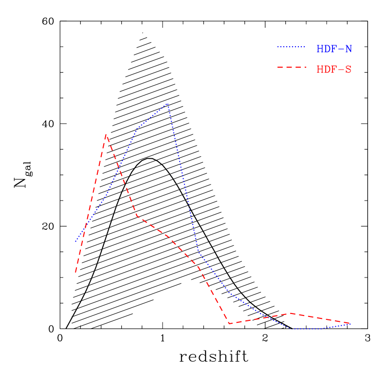
Figure 1: Redshift number counts in the Hubble Deep Fields North and South (blue dotted and red dashed lines respectively) for a magnitude cut $m_{I}=24.5$. The solid lines show the average number counts from the high galaxy density mock catalogue in a calibration survey of $5.3$ arcmin square (i.e. matching the HDF area). The gray area show the measured r.m.s. in the high density mock catalogue.

The redshift distribution in each mock field follows the input form, Eq. (5), quite well but large fluctuations, driven by the spatial clustering of galaxies (large-scale structure), are clearly visible. As we average over the different mock fields these fluctuations average away, but the field-to-field fluctuations are far larger than the Poisson error in the counts would predict [28]. Figure 1 shows the HDF North and South number counts (solid lines) for an AB magnitude cut at $m_{I}=24.5$, which is the typical limiting magnitude of most existing and many of the planned lensing surveys. Each HDF field is $5.3$ arcmin square. This figure shows that a $5.3$ arcmin square calibration survey from the mock catalogue gives similar number counts to the HDFs. Given the large error, resulting from the small HDF survey area, we conclude that our mock catalogues provide a statistical description of reality that is sufficient for the purposes of this paper.

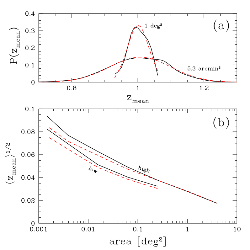
Figure 2: Top panel: the average source redshift obtained from al the fitted $n(z)$ (dark solid lines). Red dashed lines show the best Gaussian fit to the solid lines. The distribution of the average source redshift distribution directly measured from the mock catalogues is very similar to the dark solid lines. The narrow distribution corresponds to a one square degree survey. The broad distribution corresponds to a $5.3$ arcmin square (HDF) survey area. Bottom panel: The error in the average source redshift distribution as a function of the mock calibration sample area. The top two lines are for the high redshift, high number density, mock galaxy catalogue. The two bottom lines for the low redshift low number density case. The dark solid lines are from the fitted n(z) and the red dashed lines are directly measured in the mock catalogues.

Top panel of Figure 2 shows the average source redshift measured from the catalogues and from the fitted $n(z)$. The dotted lines indicate that the average redshift is well described by a Gaussian distribution, which we assume in the analysis that follows. Note that the average redshift (as shown in Figure 2) and the variance (not shown) of the fit to n(z) are not affected by the choice of the parametrization Eq.(5).

3 Results

3.1 Redshift sample variance and co-variance

A first estimation of the uncertainty introduced into cosmological parameter estimation by the redshift sampling error is given by the scatter of the measured mean redshift in the mock calibration samples. The bottom panel of Figure 2 shows the r.m.s. of the mean redshift with respect to the true average redshift for different calibration sample areas, assuming contiguous survey coverage. The top two lines correspond to the mock catalogue with mean redshift of $1.0$ and it shows the scatter of the mean redshift for the fitted distribution (solid line) and the distribution measured directly from the mock catalogues (dashed line). The bottom two lines show the same but for the lower redshift mock catalogue z=0.7. On average, the input values $\alpha=2$ and $\beta=2$ are recovered, but there are significant field-to-field variations. This comparison shows that the solid and dashed lines almost overlap, meaning that the fitting procedure does not introduce a significant excess of scatter. It also shows that the sampling error is only slightly changed between the two different mock catalogues. Interestingly, we observe that a even a 4 square degree redshift sample gives a mean redshift precision of $\sim 2$%. This corresponds roughly to an uncertainty in $\sigma_{8}$ at the same level (as illustrated by Eq.3). It is also interesting to note that the uncertainty of the mean redshift measured for a one square degree field is in agreement to the dispersion measured in the photometric redshift distribution in the four, one square degree, CFHTLS deep fields [29]. A detailed analysis of the redshift sample requirements and the resulting effect on the measurement of $\sigma_{8}$ is given in Sections 4 and 5. It should be noted here, however, that the largest complete spectroscopic redshift calibration samples that will be available for the next few years are limited to magnitude $m_{I}\simeq 24$ (VVDS and DEEP2 Groth Strip) totaling $\sim 2.5$ square degrees. These redshift surveys are clearly not big enough to calibrate the future lensing surveys that will image hundreds of square degrees with the expectation of achieving sub-percent accuracy on the measurement of cosmological parameters.

Figure LABEL:fig:zsource_rms_vs_area demonstrates that it is particularly inefficient to calibrate the redshift distribution with a large contiguous redshift survey: the precision of 3% on the mean redshift with a one square degree survey is attainable with only 10 independent HDF-sized redshift surveys (totaling 0.015 square degrees), because the error decreases as square root of the number of independent fields. This conclusion agrees with [5] who found that only a small number of spectroscopic redshifts are needed in order to calibrate a redshift distribution: the authors found that only a thousand redshifts are necessary to get the required redshift accuracy for lensing studies on nearly the whole sky. This is true if we do not worry about galaxy selection (from color, type, morphology, etc…), meaning that the calibration sub-field could be as small as we want (reduced to a single object as stated in [5]). We find that this statement is still valid even when non-linear source clustering is included, which clearly demonstrates that the number of independent calibration fields is much more important than the size of the calibration fields themselves.

Figure 3: Redshift distribution covariance matrices for different calibration survey size. From top-left to bottom-right (reading ordering) the survey size is 4 sq.deg., 1 sq.deg., 0.25 sq.deg., 225 sq.arcmin, 56 sq.arcmin and 16 sq.arcmin. For small area calibration samples, the covariance matrix becomes diagonal although the error is larger than Poisson statistics would imply (see Figure 4).

Figure 3 shows the covariance matrix of the galaxy counts in ten redshift bins between $0<z<2.3$ for six different calibration sample sizes. Small sample sizes show little correlation between bins, but the fluctuation amplitude is much larger than Poisson statistics would imply. This is shown in Figure 4 which plots the observed variance to the Poisson prediction. Even for a 16 square arcmin redshift sample the noise is 5 times the Poisson expectation! This largely explains the significant difference between the redshift number counts of the two HDFs. The decline of the sample variance r.m.s over Poisson error at large redshifts is as result of probing more uncorrelated structures as the survey volume grows.

Figure 4: Top panel: the solid lines show the ratio between the sample variance r.m.s. and the Poisson error r.m.s. From top to bottom, the lines correspond to the calibration surveys of size 4 sq.deg., 1 sq.deg., 0.25 sq.deg., 225 sq.arcmin, 56 sq.arcmin and 16 sq.arcmin respectively. Bottom panel: lines show the fractional sampling error (sample r.m.s. counts over the counts) for the same six calibration surveys where the bottom dashed line corresponds to the 4 sq.deg. calibration survey, and the top dashed line corresponds to the 16 sq.arcmin calibration survey.

3.2 The Impact on Cosmic Shear Analysis

In this section, we directly investigate the effect of the redshift sample variance on cosmological parameters measurements. We focus on the constraints on $\sigma_{8}$ and $\Omega_{m}$, since they are the main parameters that weak lensing is sensitive to (see Eq.3). As described in Section 2.3, for each mock catalogue, we have many sub-catalogues of different sizes. We have a measure of the values of $\alpha$, $\beta$ and $z_{s}$ in each of the sub-catalogues which we use to compute the covariance matrix of the shear top-hat variance $\langle\gamma^{2}\rangle$, holding the mass power spectrum $P(k)$ fixed to its theoretical value. The result is averaged over the different mock catalogue realizations. In this way, we directly obtain the contribution of the redshift sample variance to the shear covariance matrix ${\bf C_{z}}$, in other words, this corresponds to an increased error in the shear measurement due to the n(z) sampling error. The full shear covariance matrix is then given by ${\bf C}={\bf C_{s}}+{\bf C_{n}}+{\bf C_{z}}$, where ${\bf C_{s}}$ is the cosmic variance (calculated according to [30], which does include non-linear amplitude of the power spectrum, but not the non-Gaussian statistics) and ${\bf C_{n}}$ is the statistical noise. A maximum likelihood calculation of the parameters $\sigma_{8}$ and $\Omega_{m}$ is performed, assuming a fiducial model with $\Omega_{m}=0.3$, $\Omega_{\Lambda}=0.7$, $\sigma_{8}=0.9$ and a power spectrum shape parameter $\Gamma=0.21$. The fiducial source redshift distribution is given by Eq. 5. The likelihood function is given by

$$L\propto{\rm Exp}\left(-{1\over 2}d^{\rm T}~{}{\bf C}^{-1}~{}d\right),$$ (6)

where $d=\langle\gamma^{2}\rangle-\langle\gamma^{2}\rangle_{\rm fiducial}$ is the measured shear top-hat variance as function of scale minus the fiducial model top-hat variance. $d$ is given in the scale range $[0.4,140]$ arcmin, which covers the scales of interest where the effect of redshift distribution sampling variance is important.

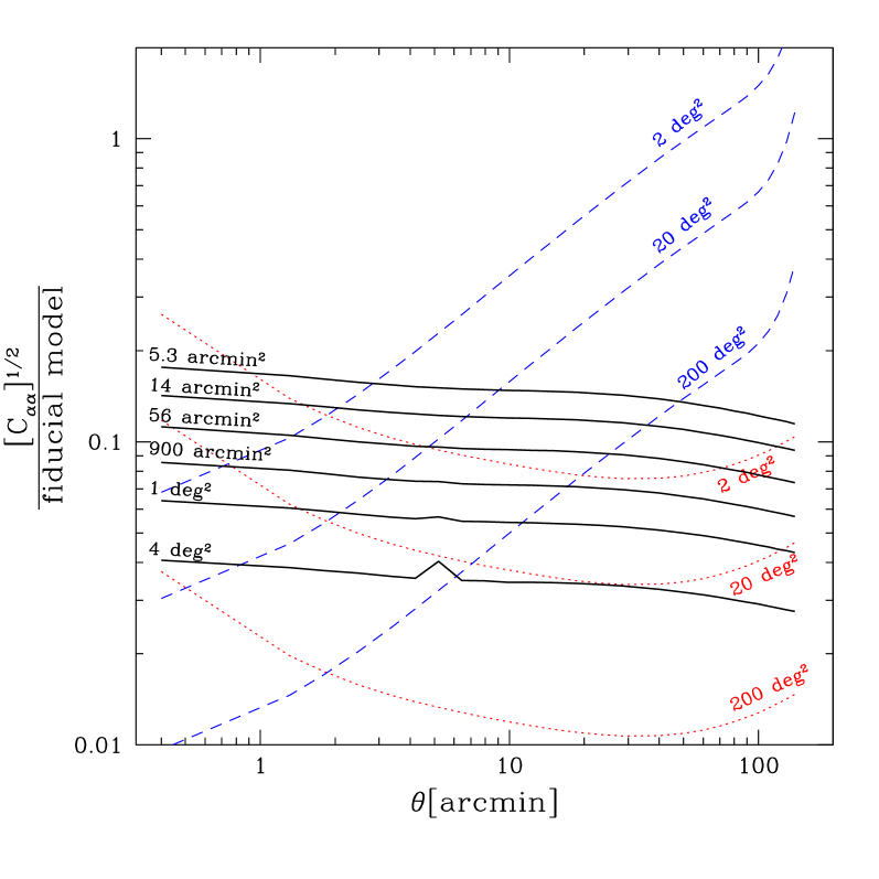
Figure 5: Different error contributions to the total lensing covariance matrix as function of the smoothing scale $\theta$. Each contribution is plotted as square root of the diagonal elements of the matrix over the signal of the fiducial model. Red dotted lines and blue dashed lines show the statistical noise and cosmic variance (along the diagonal of the covariance matrix) respectively. From top to bottom, the lines correspond to lensing surveys of size 2 sq.deg, 20 sq.deg. and 200 sq.deg. The intrinsic ellipticity is chosen to be $\sigma_{e}=0.36$ with the number density of galaxies set to 20 galaxies per arcmin square. The dark solid lines show the diagonal covariance matrix due to source redshift sample variance. From top to bottom, the redshift calibration sample is 5.3, 14, 56, 900 arc-minutes, 1 and 4 square degrees respectively.

The behavior of the redshift distribution sampling variance is particularly interesting as, to first approximation, it behaves like an unknown normalization constant in the power spectrum, as expected from Eq.3 for a single source redshift. For a broad redshift distribution, this is rather unexpected, however, as different realizations of redshift distribution can vary greatly for different lines-of-sight, changing not only the mean source redshift but the entire shape of the distribution as well. We find that the main contribution of the redshift sample variance can be characterized by an effective mean source redshift, as if the sources were located in a single redshift plane. Figure 5 shows that this is not the case to second order, where the r.m.s. of the ratio between the diagonal elements of the sampling variance covariance matrix and the fiducial model shows a slight dependence on the smoothing scale. The off-diagonal components, not shown here, are such that the correlation coefficient over the entire matrix is $\sim 1$ within $2\%$ accuracy. Therefore, the redshift uncertainty is mostly degenerate with $\sigma_{8}$ and with a shear calibration error, which is defined as the factor $1\pm\epsilon$ between the observed $\gamma_{\rm obs}$ and true shear $\gamma_{\rm true}$, such that $\gamma_{\rm obs}=(1\pm\epsilon)\gamma_{\rm true}$ . A shear calibration error can arise from a galaxy shape measurement error which is quantified in [4]. With this knowledge, it is then easy to include the redshift sampling variance caused by non-linear large scale structures in parameter forecasts by simply increasing the uncertainty in the shear calibration factor. Another interesting feature of Figure 5 is that the n(z) sample variance has the largest impact in the scale range $[1,10]$ arc-minutes (although it largely depends on the survey type), where the sum of the two main sources of error in cosmic shear surveys reaches a minimum. Above a few tens arcminutes, the cosmic variance dominates, below one arcminute, the shot noise becomes dominant (note that in this figure the intrinsic ellipticity distribution is chosen to be $\sigma_{e}=0.36$ with the number density of galaxies set to 20 galaxies per arcmin square). The optimal redshift calibration survey would then be designed such that its contribution to the shear covariance never exceeds the value of the crossing point between the statistical and cosmic variance errors. Changing the survey characteristic numbers will change the redshift calibration requirements. A detailed discussion on survey design including the redshift calibration issue is included in the next Section.

4 Designing future lensing surveys

4.1 Statistical noise versus cosmic variance

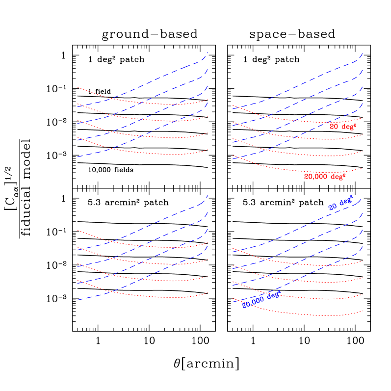
Figure 6: The different sources of noise for ground-based (left panels) and space-based (right panels) lensing surveys, normalized to the fiducial model. The dark solid lines show the diagonal of the redshift sampling covariance matrix, from top to bottom they correspond to a calibration sample with $1$, $10$, $100$, $1000$, $10000$ fields, assuming a sparse survey, each field is a one sq.deg. patch (top panels) and $5.3$ arcmin square patch (bottom panels). The blue dashed lines show the cosmic variance and the red dotted lines the statistical noise for four lensing surveys sizes. From top to bottom the lines correspond to lensing surveys of $20$, $200$, $2000$, $20000$ sq.deg.. The ground based survey (left panels) assumes a galaxy number density $n_{gal}=15$ per arcmin square and shape noise $\sigma_{e}=0.44$, while the shallow space based survey (right panels) assumes $n_{gal}=35$ and $\sigma_{e}=0.36$.

We now turn to forecasting to make predictions regarding the minimal requirements for redshift calibration surveys. As it was mentioned previously, we want the redshift sample variance noise to be, at most, equal to the crossing point of the cosmic variance and statistical noise errors. This constraint sets the size of the needed calibration survey for a fixed set of lensing survey characteristics. The best approach is to make a sparse calibration survey (see Section 3.1) in order to minimize the sample variance between the different fields. Therefore we adopt the following strategy: we assume that the redshift calibration survey is made of a collection of $N_{\rm cal}$ uncorrelated redshift (spectrometric or photometric) surveys. The size of the individual patches is either one square degree or $5.3$ square arcmin (HDF size), from which we compare the performance. The error on the mean redshift scales as $\sqrt{N_{\rm cal}}^{-1}$, with a redshift uncertainty of nearly $3\%$ for the one sq.deg. patch and $9\%$ for the $5.3$ arcmin square (see Figure 2). We consider four lensing surveys of size $(20,200,2000,20000)$ square degrees, and five redshift calibration surveys of $(1,10,100,1000,10000)$ fields (sparsely sampled with patches of one square degree or 5.3 square arc-minutes each). We also consider a ground-based type of statistical noise, with a number density of galaxies per arcmin square $n_{gal}=15$ and an ellipticity noise $\sigma_{e}=0.44$, and a shallow space-based type of statistical noise with $n_{gal}=35$ and $\sigma_{e}=0.36$ (consistent with DUNE [31]).

Figure 6 compares the different noise amplitudes for the different surveys. It is interesting to note the difference between ground and space based surveys. If we assume one square degree calibration patches, then a $20000$ sq.deg. ground based survey can be calibrated with a $1000$ square degree redshift survey, however this is clearly not good enough for the $20000$ square degrees space based survey, which will not perform significantly better than a $2000$ square degrees survey if the calibration sample is not increased to $10000$ sq.deg. This discussion is particularly relevant if we want to measure the cosmic shear power spectrum in the $1-10$ arcmin range. One could imagine a ground based $10$ sq.deg. calibration redshift survey, for example, which would already be very time consuming if the goal was to match space-based lensing data in terms of depth and galaxy number density. The redshift sampling errors resulting from the small size of the calibration survey would effectively wash out the lensing signal producing results similar to a $200$ sq.deg. lensing survey for scales below $2$ arcmin and $2000$ sq.deg. for scales between $2$ and $10$ arcmin. If the calibration patch is only $5.3$ arcmin square (HDF area), the same redshift accuracy is reached for patches of one square degrees with only ten times more independent fields, even though the HDF is nearly $700$ times smaller than one square degree.

This analysis also demonstrates that one cannot separate the issue of redshift calibration and shear calibration. Both need to be below the sum of the statistical and cosmic variance errors in order for the lensing survey to be fully efficient. As we can see from Figure 6, a shear calibration error of $1\%$ would dramatically limit the cosmological information that can be extracted from a lensing survey larger than 200 square degrees, and any improvement in redshift calibration below that limit would indeed be a waste of observing time, unless the shear calibration is also improved. This is consistent with [5] who discuss why it is useless to improve either redshift error or the shear calibration. Figure 6 shows that both have to be below the sum of statistical and cosmic variance errors if we want the lensing survey to deliver its full potential. It is worth noting that this discussion also applies to the self calibration regime proposed by [6] in which the shear calibration is treated as a free parameter included with the cosmological parameters we want to measure. Self calibration could however allow us, by combining second and third order shear statistics, to reach higher calibration precision than the shape measurement accuracy.

The conclusion of this section is that there is a tight relation between the source redshift sampling variance, the shear calibration error and the statistical noise of a lensing survey, the later being determined by the survey characteristics. This relation is important for the design of lensing surveys. For instance if the combined redshift and shear calibration errors are at the $1\%$ level, then a $20000$ square degrees space based lensing survey with $35$ galaxies per arcmin square would do as well as if the number density of galaxies was only $0.35$ per arcmin square.

4.2 Calibration requirements for future lensing surveys

In the previous section, we demonstrated that the accuracy of the shear calibration sets strong limits on the ability of lensing surveys to probe small angular scales $\theta<30$ arcmin. Although the shear calibration error has been included in cosmological parameter forecasts as an unavoidable source of systematics [6], to date, there has been no discussion on how shear calibration could limit the design of a lensing survey. In this section we therefore try to answer this question by comparing a large sample of observing strategies, and derive the shear calibration requirement for each of them. Note that we will refer generically to ‘shear calibration’ when talking about redshift or shear calibration errors, since, to first approximation, they impose the same limitation to a lensing survey. Our analysis will result in a tight relation between the shear calibration accuracy and the best lensing survey that one can undertake, beyond which accumulating more data would not improve anything unless the shear calibration is itself improved.

To model the redshift distribution $n(z)$ of different magnitude limited surveys (i.e with $m<m_{\rm lim}$) we use the method described in [18], such that

$$n(z)\left[m<m_{\rm lim}\right]={\sum_{i=1}^{\rm lim}N(i)n(z,m_{i})\over\sum_{i=1}^{\rm lim}N(i)}$$ (7)

where $n(z,m_{i})$ is the redshift distribution of galaxies in magnitude slice of width $\Delta m=0.5$ with a maximum magnitude $m_{i}$, and $N(i)$ is the number density of resolved galaxies in each magnitude slice. We model $n(z,m_{i})$ using equation(5) with $\alpha=2.2$ and $\beta=1.0$, corresponding to the best-fitting shape parameters to the HDF photometric redshift distribution from [32]. Using these parameters $z_{0}=z_{m}/2.87$ where the median redshift $z_{m}$ can be estimated from the redshift-magnitude relation of [18] ($z_{m}=-3.132+0.164m$ where the AB magnitude $m$ is for the F606W HST filter). We estimate the number density of resolved galaxies in each magnitude slice $N(i)$ from the galaxy number counts in the HST ultra-deep field , considering two different cases; a ground-based survey with 0.7 arcsec seeing and a deep space-based survey (e.g. SNAP) where the resolution is limited by 0.1 arcsec pixels. We define a source to be adequately resolved for lensing studies if the object’s half light radius is greater than the resolution limit set by the atmospheric seeing (ground), or pixel scale (space). Table 1 lists the resulting number density of sources and median source redshift for ground and space-based surveys with different limiting magnitudes. One should be careful here as these numbers were obtained from a small field-of-view and are therefore sensitive to the sampling variance discussed in this paper, this explains why the brightest magnitude counts appear deeper (in redshift) from the ground than from space. However, what is important for our purpose here, is the relative evolution of the statistical noise and cosmic variance as function of redshift.

Using this model, we calculate the covariance and statistical noise matrices for ground and space based surveys, with limiting magnitudes between $m_{\rm\lim}=24.5$ and $m_{\rm\lim}=28.5$. The left panel of Figure 7 shows that the covariance matrix is relatively insensitive to the survey limiting magnitude: surveys with very different $m_{lim}$ will have very different lensing signal amplitude, but the covariance matrix will scale accordingly. The covariance roughly scales as the inverse of the survey area. This means that the efficiency of the different limiting magnitude surveys will essentially differ by the change in the statistical noise contribution to the covariance matrix, the ratio of the cosmic variance to the lensing signal remaining the same.

With the data from Table 1 we calculate the top-hat shear variance for different models, and define the shear calibration requirement as the particular point where the diagonal elements of the cosmic variance and statistical noise matrices divided by the signal cross each other. The right panel of Figure 7 shows the shear requirement as function of the limiting magnitude and angular scale of the lensing survey plotted along with some of the planned lensing surveys (LSST, DUNE [31] and SNAP).

We fit the shear calibration requirement to the magnitude and survey size from Figure 7 and find that the shear calibration $\epsilon$ (see Section 3.2) must be below $\epsilon=\epsilon_{0}10^{\beta(m-24.5)}\left(\Theta\over 200\right)^{-1/2}$, where $(\epsilon_{0},\beta)=(0.015,-0.18)$ and $(\epsilon_{0},\beta)=(0.011,-0.23)$ for a ground and space based survey respectively. The $\Theta$ dependence of this limit is driven by the cosmic variance only (consistent with [6]), while the magnitude dependence is driven by the statistical noise via the number counts.

Table 1: Table showing the average source redshift and galaxy number density for different limiting magnitude surveys where the calculation is described in the text. The survey limiting F606W AB magnitudes are given in the first column, the average source redshift in the second, and the last column is the number density of galaxies per arc-minute square. The quoted numbers correspond to a ground (space) based survey.

Survey depth	$\langle z_{source}\rangle$	$n_{gal}$
24.5	0.825 (0.787)	8 (13)
25.0	0.879 (0.869)	11 (20)
25.5	0.951 (0.948)	16 (30)
26.0	1.019 (1.044)	21 (45)
26.5	1.076 (1.128)	26 (65)
27.0	1.143 (1.216)	32 (91)
27.5	1.196 (1.285)	38 (124)
28.0	1.248 (1.358)	44 (166)
28.5	1.307 (1.440)	51 (222)

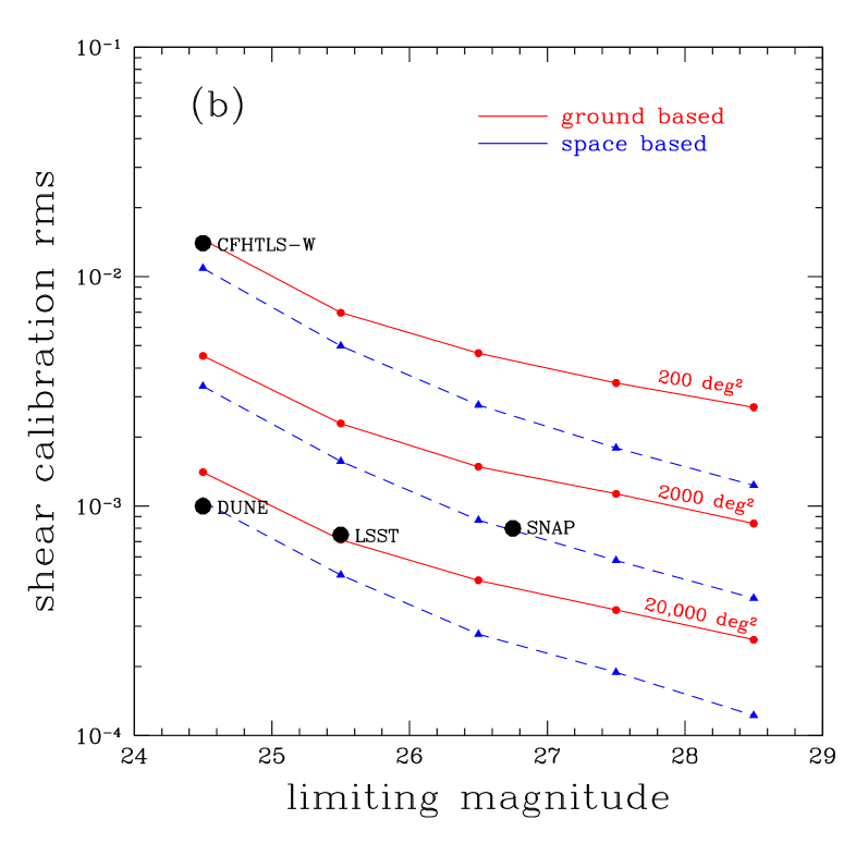
Figure 7: Left panel: the cosmic variance contribution for different survey sizes. There are three curve bundles, from top to bottom the curves correspond to survey sizes $200$, $2000$ and $20000$ square degrees. In each bundle, the lines correspond to different limiting magnitudes: 24.5, 25.5, 26.5, 27.5, 28.5. Right panel: each line shows the calibration requirement for different survey strategies, calculated as explained in Section 4.2. The plot shows the optimal calibration r.m.s. for ground and space based surveys with different depths. The dark bullets display some the future and present weak lensing surveys.

5 A note regarding previous cosmic shear measurements

Given that the impact of redshift sampling variance has so far been neglected, and that nearly all present lensing surveys rely on the HDFs to calibrate their redshift distribution, one should investigate whether the errors on published cosmic shear measurements have been correctly estimated. Table 2 shows the error on the normalization of the power spectrum $\sigma_{8}$ for different surveys where the redshift calibration sample consists of two independent HDF-sized surveys. One can see that for a lensing survey such as VIRMOS or CFHTLS-WIDE in its present stage, although the redshift uncertainty is large, the difference between assuming a Poisson redshift distribution or the full sample covariance is only at the $\sim 10$ percent level. This is not true for deeper surveys of the same size (e.g model (20,1.0) in table 2), where the difference can be as large as $100$%, as well as for the complete 200 square degree CFHTLS-WIDE survey. The multi-color data of the CFHTLS will be crucial in order to produce complete photometric redshift catalogues and thus achieve the cosmic variance limited accuracy. According to Figure 7, one also needs to achieve a shear calibration accuracy of one percent which is the current state of the art of weak shear measurement [4].

The recent third year WMAP release [33] has shown that $\sigma_{8}$ measured from CFHTLS [10, 11] is rather on the high side. The redshift sample variance discussed in this work could easily account for this difference: the HDFs have been chosen as empty fields, and it is not unreasonable to believe that their redshift distribution could significantly differ from the average distribution as a consequence of selection effects. One should also note that COMBO-17 [17] found a relatively low $\sigma_{8}$, fully consistent with [33], using accurate redshift information. Fortunately, the CFHTLS survey will soon deliver photometric redshifts for the DEEP [29] and WIDE surveys and it will become possible to calibrate the redshift distribution to the accuracy required by the size of the lensing data set. Future work will include a preliminary check of the CFHTLS results with the CFHTLS DEEP photometric redshifts [29] and a lensing analysis that combines all surveys published to date, taking into account a more realistic redshift distribution than the previously used Hubble Deep Fields. In [34], it was mentioned that the RCS photometric redshifts show that the actual mean redshift is larger than the one from HDF. The RCS $\sigma_{8}$ should probably be about $8\%$ lower. This is another good example why photometric redshifts are essential.

Table 2: Table indicating the error on the measured $\sigma_{8}$ with two independent HDF sized samples as the redshift calibration survey. The second column assumes Poisson error for the redshift distribution plus cosmic variance. The third column is for the full redshift sample variance and cosmic variance, and the last column assumes cosmic variance only. The first column specifies the lensing survey type, where the first number indicates the area in square degrees and the second number indicates the mean source redshift. The number density of galaxies is always $15$ galaxies per arc-minute square, which represents an average number count for sources between redshift 0.7 and 1., and the shape noise is $0.44$, these numbers correspond to a typical ground based survey for these redshift depth.

model	$\Delta_{Poiss}\sigma_{8}$	$\Delta_{All}\sigma_{8}$	$\Delta_{Covar}\sigma_{8}$
(4,0.7)	0.136	0.143	0.098
(20,0.7)	0.084	0.092	0.037
(200,0.7)	0.051	0.063	0.013
(4,1.0)	0.058	0.077	0.056
(20,1.0)	0.030	0.057	0.025
(200,1.0)	0.018	0.046	0.008

6 Conclusions

We have studied the effect of redshift sample variance on cosmic shear measurements using a realistic distribution of galaxies embedded in dark matter halos. This source of error occurs when photometric redshifts cannot be obtained for the entire lensing survey, which is the case for all current surveys, and will be the case for some of the future surveys that will be unable to follow up in multi-color all of the fainter galaxies that will be used in the lensing analysis. We derived what minimum requirements a redshift calibration sample should have in order to make the redshift distribution error negligible compared to the statistical and cosmic variance errors. We have shown that the redshift sample variance behaves like a shear calibration factor to first approximation, even for the general case when galaxies are distributed within large scale structures. We have shown that even when non-linear source clustering is included, the best redshift sampling strategy is still a sparse sample. However it is clear that the best way to avoid redshift sampling issues is to have a complete photometric redshift survey, which is also required to remove contamination from intrinsic galaxy alignments (see for example [35]) and shear-ellipticity correlations [36, 37].

The shear and redshift calibrations are both important for designing future lensing surveys. An optimal use of lensing survey time is to guarantee that the statistical and cosmic variance errors are not smaller than the summed redshift and shear calibration errors. This is particularly critical for small angular scales (less than a few tens arcminutes), and it puts strong constraints on the useful maximum galaxy number density a lensing survey should have. We have derived the calibration requirements using realistic galaxy number counts from the Hubble Ultra-Deep Field.

Among the work that remains is to investigate how the photometric redshift errors couple to the sampling variance error. A more realistic analysis will also include realistic galaxy populations with color, morphology and size distributions. Our analysis will also have to be extended to include tomography studies. Some recent papers discuss the effect of imperfect photometric measurement on cosmic shear studies in the tomographic case [6, 7]. The authors allow for different error models in the estimated mean redshift and they concluded that the mean redshift must be known to great accuracy, a few $10^{-3}$, which is similar to our calibration requirement for almost full sky surveys.

Future lensing surveys are designed such that the number density of source galaxies is higher than the current value of $\sim 20$ galaxies per arc-minute square. That means they have the ambitious goal of measuring the mass power spectrum at a relative precision of $10^{-3}$. This is clearly possible only if both the source redshift and the shear calibration errors are known to a similar accuracy, a level of precision which is still far below the actual state of the art of weak shear measurement [4].

We thank Mustapha Ishak-Boushaki for discussions on the topics developed in this work, Eric Linder, Dragan Huterer and Gary Bernstein for useful comments on the manuscript and Alexandre Réfrégier for discussions regarding the DUNE project. We are very grateful to Tamas Budavai for sharing his HDF photometric redshift catalogues and the full probability distributions for each object. The simulations used here were performed on the IBM-SP at NERSC. MJW was supported in part by NASA and the NSF. This work uses data from the Hubble Ultra Deep Field (UDF) which is a public HST survey made possible by Cycle 12 STSci Director’s Discretionary Time, programme GO/DD-9978. LVW and HH are supported by the Natural Sciences and Engineering Research Council (NSERC), the Canadian Institute for Advanced Research (CIAR) and the Canadian Foundation for Innovation (CFI), CH is supported by a CITA National Fellowship, NSERC and CIAR.

References

- [1] Y. Mellier, Ann. Rev. Astron. Astrophys., 37, 127 (1999); M. Bartelmann, P. Schneider, Phys. Rep., 340, 291 (2001).
- [2] L. van Waerbeke, Y. Mellier, Lectures given at the Aussois winter school, January 2003 [astro-ph/0305089].
- [3] H. Hoekstra, H.K.C. Yee, M.D. Gladders, New Astronomy Reviews, 46, 767 (2002).
- [4] C. Heymans, et al., preprint [astro-ph/0506112].
- [5] M. Ishak, C. Hirata, PhRev, D71, 023002 (2005).
- [6] Huterer, D., Takada, M., Bernstein, G., Jain, B., 2006, MNRAS, 366, 101.
- [7] Ma, Z., Hu, W., Huterer, D., 2006, ApJ, in press, astro-ph/0506614.
- [8] Van Waerbeke, L., Mellier, Y., Hoekstra, H., A& A, 429, 75
- [9] Hoekstra, H., Yee, H., Gladders, M., ApJ, 2002, 577, 595
- [10] Hoekstra, H., et al., ApJ, 2006, astro-ph/0511089, in press
- [11] Semboloni, E., et al. A& A, 2006, astro-ph/0511090, in press
- [12] R. Massey, et al., MNRAS, 359, 1277 (2005).
- [13] J. Rhodes, A. Refregier, E.J. Groth, ApJ, 552, L85 (2001).
- [14] A. Refregier, J. Rhodes, E.J. Groth, ApJL, 572, L131 (2002)
- [15] J. Rhodes, et al., ApJ, 605, 29 (2004); H. Hammerle, et al., A&A, 385, 743 (2002); J.-M. Miralles et al., A&A, 432, 797 (2005).
- [16] Williams, R.E., Blacker, B., Dickinson, M., et al., 1996, AJ, 112, 1335; Fernández-Soto, A., Lanzetta, K.M., Yahil, A., 1999, ApJ, 513, 34; Cohen, J., Hogg, D., Blandford, R., et al., 2000, ApJ, 538, 29
- [17] Brown, M. L, et al., MNRAS, 341, 100 (2003)
- [18] Heymans, C., Brown, M. L and Barden, M., Caldwell, J. A. R. et al., 2005, MNRAS, 361, 160
- [19] O. Le Fèvre, et al., A&A, 439, 845 (2005).
- [20] M. Davis, et al., Proc. SPIE, 4834, 161 (2003).
- [21] Bernardeau, F., Van Waerbeke, L., Mellier, Y., 1997, A& A, 322, 1
- [22] M. White, ApJS, 143, 241 (2001).
- [23] M. Davis, G. Efstathiou, C.S. Frenk, S.D.M. White, ApJ, 292, 371 (1985).
- [24] K. Abazajian, et al., ApJ, 625, 613 (2005).
- [25] C. Conroy, R.H. Wechsler, A.V. Kravtsov, preprint [astro-ph/0512234]
- [26] R. Yan, M. White, A. Coil, ApJ, 607, 739 (2004);
- [27] J. Navarro, C.S. Frenk, S.D.M. White, ApJ, 490, 493 (1997).
- [28] P.J.E. Peebles, “Large-scale structure of the Universe”, Princeton University Press (1980).
- [29] Ilbert, O., Arnouts, S., McCraken, H., et al. 2006, astro-ph/0603217
- [30] P. Schneider, L. van Waerbeke, M. Kilbinger, Y. Mellier, A&A, 396, 1 (2002).
- [31] Réfrégier, A., private communication
- [32] Budavári, T., Szalay, A. S., Connolly, A. J., Csabai, I., Dickinson, M., ApJ, 120, 1588, (2000)
- [33] Spergel, et al., 2006, astro-ph/0603449, WMAP third year release http://lambda.gsfc.nasa.gov/product/map/current/map_bibliography.cfm
- [34] Hoekstra, H., et al., ApJ, 2005, 635, 73
- [35] King, L., Shneider, P., A& A, 2002, 396, 441; Heymans, C., Heavens, A., MNRAS, 2003, 339, 711; Takada, M., White, M., ApJ, 2004, 601, L1
- [36] King, L., A&A, 2005, 441, 47
- [37] Heymans, C., White, M., Heavens, A., Vale, C., Van Waerbeke., 2006, MNRAS submitted, astro-ph/0604001