Cross-correlation of WMAP 3rd year data and the SDSS DR4 galaxy survey: new evidence for Dark Energy

Abstract

We cross-correlate the third-year WMAP data with galaxy samples extracted from the SDSS DR4 (SDSS4) covering 13% of the sky, increasing by a factor of 3.7 the volume sampled in previous analysis. The new measurements confirm a positive cross-correlation with higher significance (total signal-to-noise of about 4.7). The correlation as a function of angular scale is well fitted by the integrated Sachs-Wolfe (ISW) effect for LCDM flat FRW models with a cosmological constant. The combined analysis of different samples gives $\Omega_{\Lambda}=0.80-0.85$ (68% Confidence Level, CL) or $0.77-0.86$ (95% CL). We find similar best fit values for $\Omega_{\Lambda}$ for different galaxy samples with median redshifts of $z\simeq 0.3$ and $z\simeq 0.5$, indicating that the data scale with redshift as predicted by the LCDM cosmology (with equation of state parameter $w=-1$). This agreement is not trivial, but can not yet be used to break the degeneracy constraints in the $w$ versus $\Omega_{\Lambda}$ plane using only the ISW data.

1 Introduction

Dark Energy (DE) models with late time cosmic acceleration, such as the $\Lambda$-dominated CDM model, predict a slow down for the growth of the linear gravitational potential at moderate redshift $z<1$, which can be observed as temperature anisotropies in the CMB: the so-called late integrated Sachs-Wolfe (ISW) effect. The ISW effect is expected to produce an increase of power (a bump) in the amplitude of the CMB fluctuations at the largest scales, ie lower order multipoles, which are dominated by cosmic variance. This expectation, seems challenged by observations, as the first year WMAP results (WMAP1) confirmed the low amplitude of the CMB quadrupole first measured by COBE (eg Hinshaw et al. 1996a). The discrepancy between the observations and the $\Lambda$CDM model is particularly evident in the temperature angular correlation function $w_{2}(\theta)$, which shows an almost complete lack of signal on angular scales $\theta\lower 2.15277pt\hbox{$\;\buildrel>\over{\sim}\;$}60$ degrees. According to Spergel et al. (2003), the probability of finding such a result in a spatially-flat $\Lambda$CDM cosmology is about $1.5\times 10^{-3}$. This was questioned in Gaztañaga et al. (2003) who found, using simulated $\Lambda$CDM WMAP maps, a much lower significance (less than 2-sigma) for $w_{2}(\theta)$. A low significance was also estimated by different studies (eg Efstathiou 2003, Olivera-Costa et al. 2003), although a discrepancy larger than 3-sigma still remains on both the quadrupole-octopole alignment (Tegmark, Oliera-Costa & Hamilton 2003, Olivera-Costa et al. 2003) and the WMAP observed high value of the temperature-polarization cross-correlation on large scales (Doré, Holder & Loeb 2004).

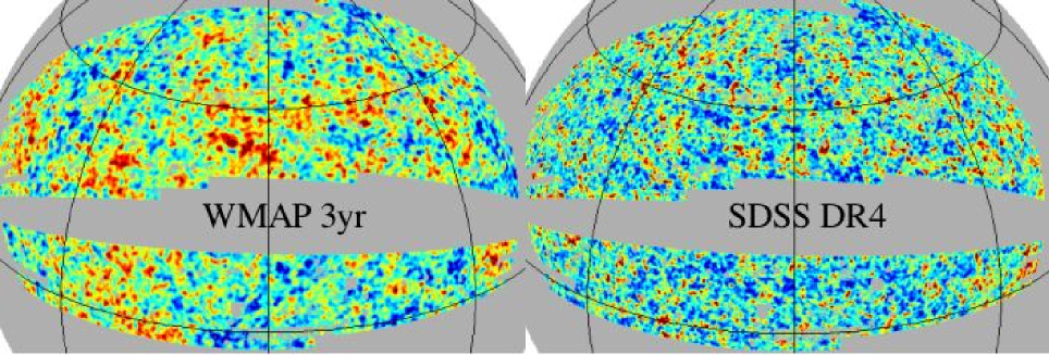
Figure 1: SDSS DR4 galaxy density (LRG) fluctuation maps (right panel) compared to WMAP (V-band 3yr) temperature map (left panel). Both maps are smoothed with a Gaussian beam of FWHM $=0.3$ deg.

Given the observed anomalies on the ISW predictions, it is of particular interest to check if the ISW effect can be detected observationally through an independent test, such as the cross-correlation of temperature fluctuations with local tracers of the gravitational potential (?). A positive cross-correlation between WMAP1 and galaxy samples from the Sloan Digital Sky Survey (SDSS) was first found by Fosalba, Gaztañaga & Castander (2003, FGC03 from now on) and Scraton et al. (2003). FGC03 used the 1yr WMAP data (WMAP1) and the SDSS data release 1 (SDSS1). WMAP1 has also been correlated with the APM galaxies (Fosalba & Gaztañaga 2004), infrared galaxies (?), radio galaxies (?), and the hard X-ray background (?; ?). The significance of these cross-correlations measurements was low (about 2-3 $\sigma$, see Gaztañaga, Manera & Multamäki 2006 for a summary and joint analysis), and many scientists are still skeptical of the reality of these detections. Here we want to check if these results can be confirmed to higher significance using the SDSS data release 4 (SDSS4) which covers $~{}3$ times the volume of SDSS1. At the same time, we will compare the signal of the 1st and 3rd year WMAP data (WMAP3) recently made public (?; ?). With better signal-to-noise and better understanding of foreground contamination in WMAP3, it remains to be seen whether the low significance signal of the WMAP1-SDSS1 analysis can be confirmed with WMAP3-SDSS4, or if on the contrary this signal vanishes as systematic and statistical errors are reduced.

2 The Data

In order to trace the changing gravitational potentials we use galaxies selected from the Sloan Digital Sky Survey Data Release 4 (?), SDSS4 hereafter, which covers 6670 deg² (i.e, 16$\%$ of the sky). We have selected subsamples with different redshift distributions to check the reliability of the detection and to probe the evolution of the ISW effect. All subsamples studied contain large number of galaxies, between 10⁶-10⁷, depending on the subsample. We concentrate our analysis on the North Galactic Cap SDSS4 Area ($\sim$ 5500 deg²), because it contains the most contiguous area. We have selected 3 magnitude subsamples with $r=18-19$, $r=19-20$ and $r=20-21$ and a high redshift Luminous Red Galaxy (LRG; e.g. Eisenstein et al. 2001) color selected subsample ($17<r<21$, $(r-i)>(g-r)/4+0.36$, $(g-r)>0.72*(r-i)+1.7$). Because of the smaller volume, the $r=18-19$ and $r=19-20$ subsamples provide low signal-to-noise (S/N$<$2) in the cross-correlation with WMAP, and we therefore center our analysis on the two deeper subsamples. The mask used for these data avoids pixels with observed holes, trails, bleeding, bright stars or seeing greater than 1.8.

To model the redshift distribution of our samples we take a generic form of the type:

$$\mbox{$$}N(z)\sim\phi_{G}(z)\sim(z-z_{c})^{2}~{}\exp{{\left(-{{z-z_{c}}\over{z_{0}-z_{c}}}\right)^{3/2}}},$$ (1)

for $z>z_{c}$ and zero otherwise. The $N(z)$ distribution of the $r=20-21$ subsample is quite broad with $z_{c}\simeq 0$ and $z_{0}\simeq 0.2$ which results in a median redshift, $\bar{z}=1.4z_{0}\simeq 0.3$ (e.g., Dodelson et al. 2001, Brown et al. 2003). On the other hand, the LRG subsample has a narrower redshift distribution. The first colour cut is perpendicular to the galaxy evolutionary tracks in the (g-r) .vs.(r-i) colour space and ensures that very few $z<0.40$ galaxies are selected, which translates into a cut $z_{c}\simeq 0.37$ in the above $N(z)$ model. The second colour cut is parallel to evolution and perpendicular to spectral type differences and selects only red galaxies with old stellar populations. The faint magnitude limit ($r<21$) cuts high redshift galaxies ($z_{0}\simeq 0.45$), which results in an overall median redshift of $\bar{z}\simeq 0.5$.

We use the full-sky CMB maps from the third-year WMAP data (?; ?) (WMAP3 from now on). In particular, we have chosen the V-band ($\sim 61$ GHz) for our analysis since it has a lower pixel noise than the highest frequency W-band ($\sim 94$ GHz), while it has sufficient high spatial resolution ($21^{\prime}$) to map the typical Abell cluster radius at the mean SDSS depth. We use a combined SDSS+WMAP mask that includes the Kp0 mask, which cuts $21.4\%$ of WMAP sky pixels (?), to make sure Galactic emission does not affect our analysis. WMAP and SDSS data are digitized into $7^{\prime}$ pixels using the HEALPix tessellation . Figure 1 shows how the WMAP3 and SDSS4 pixel maps look like when density and temperature fluctuations are smoothed on $0.3$ deg scale.

3 Cross-Correlation and errors

We define the cross-correlation function as the expectation value of density fluctuations $\delta_{G}=N_{G}/<N_{G}>-1$ and temperature anisotropies $\Delta_{T}=T-T_{0}$ (in $\mu$K) at two positions ${\hat{n}}_{1}$ and ${\hat{n}}_{2}$ in the sky: $w_{TG}(\theta)\equiv\langle\Delta_{T}({\bf{\hat{n}}_{1}})\delta_{G}({\bf{\hat{n}}_{2}})\rangle$, where $\theta=|\bf{{\hat{n}}_{2}}-\bf{{\hat{n}}_{1}}|$, assuming that the distribution is statistically isotropic. To estimate $w_{TG}(\theta)$ from the pixel maps we use:

$$\mbox{$$}w_{TG}(\theta)={\sum_{i,j}\Delta_{T}({\bf{\hat{n}}_{i}})~{}\delta_{G}({\bf{\hat{n}}_{j}})~{}w_{i}~{}w_{j}\over{\sum_{i,j}w_{i}~{}w_{j}}},$$ (2)

where the sum extends to all pairs $i,j$ separated by $\theta\pm\Delta\theta$. The weights $w_{i}$ can be used to minimize the variance when the pixel noise is not uniform, however this introduces larger cosmic variance. Here we follow the WMAP team and use uniform weights (i.e. $w_{i}=1$). The resulting correlation is displayed in Fig.2. On scales up to $10$ degrees we find significant correlation above the estimated error-bars. The dotted and continuous lines correspond to WMAP1 and WMAP3 data respectively, and show little difference within the errors. This indicates that the cross-correlation is signal dominated.

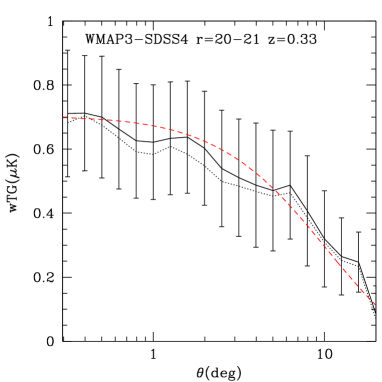
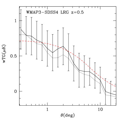
Figure 2: The continuous line with errorbars shows the WMAP3-SDSS4 angular cross-correlation as a function of scale for the $r=20-21$ sample (top) and the LRG sample (bottom). The dotted line corresponds to using the 1st yr WMAP (WMAP1-SDSS4) data, which is very close to the WMAP3 results (continuous line). The dashed lines show the $\Lambda$CDM model with $\Omega_{\Lambda}=0.83$ ( best overall fit) scaled to the appropriate bias and projected to each sample redshift.

$\theta(deg)$	$wTG(20-21)$	$wTG(LRG)$
0.316	$0.711\pm 0.198$	$0.876\pm 0.279$
0.398	$0.712\pm 0.180$	$0.793\pm 0.266$
0.501	$0.700\pm 0.190$	$0.781\pm 0.266$
0.631	$0.662\pm 0.187$	$0.724\pm 0.268$
0.794	$0.626\pm 0.179$	$0.691\pm 0.255$
1.000	$0.622\pm 0.179$	$0.606\pm 0.251$
1.259	$0.634\pm 0.176$	$0.547\pm 0.258$
1.585	$0.637\pm 0.175$	$0.602\pm 0.260$
1.995	$0.603\pm 0.178$	$0.637\pm 0.261$
2.512	$0.540\pm 0.182$	$0.552\pm 0.263$
3.162	$0.511\pm 0.183$	$0.394\pm 0.249$
3.981	$0.488\pm 0.194$	$0.298\pm 0.241$
5.012	$0.470\pm 0.188$	$0.281\pm 0.222$
6.310	$0.488\pm 0.168$	$0.277\pm 0.192$
7.943	$0.407\pm 0.172$	$0.224\pm 0.181$
10.000	$0.320\pm 0.150$	$0.158\pm 0.183$
12.589	$0.265\pm 0.121$	$-0.004\pm 0.182$
15.849	$0.247\pm 0.094$	$-0.031\pm 0.172$
19.953	$0.086\pm 0.087$	$-0.052\pm 0.128$

Table 1: $w_{TG}(\theta)$ for WMAP3-SDSS4.

We have used different prescriptions to estimate the covariance matrix: a) jack-knife, b) 2000 montecarlo simulations c) theoretical estimation (including cross-correlation signal) both in configuration and harmonic space. Our montecarlo simulations in b) include independent simulations of both the CMB and galaxy maps, with the adequate cross-correlation signal. All three estimates give very similar results for covariance and the $\chi^{2}$ errors, details will be presented elsewhere (Fosalba et al. 2006).

To compare models we use a $\chi^{2}$ test:

$$\mbox{$$}\chi^{2}=\sum_{i,j=1}^{N}\Delta_{i}~{}C_{ij}^{-1}~{}\Delta_{j},$$ (3)

where $\Delta_{i}\equiv w_{TG}^{E}(\theta_{i})-w_{TG}^{M}(\theta_{i})$ is the difference between the ”estimation” $E$ and the model $M$. We perform a Singular Value Decomposition (SVD) of the covariance matrix $C_{ij}=(U_{ik})^{\dagger}D_{kl}V_{lj}$ where $D_{ij}=\lambda_{i}^{2}\delta_{ij}$ is a diagonal matrix with the singular values on the diagonal, and $U$ and $V$ are orthogonal matrices that span the range and nullspace of $C_{ij}$. We can choose the number of eigenvectors $\widehat{w}_{TG}(i)$ (or principal components) we wish to include in our $\chi^{2}$ by effectively setting the corresponding inverses of the small singular values to zero. In practice, we work only with the subspace of “dominant modes” which have a significant “signal-to-noise” (S/N). The S/N of each eigenmode, labeled by $i$, is:

$$\mbox{$$}\Big{(}\frac{S}{N}\Big{)}_{i}=\Big{|}\frac{\widehat{w}_{TG}(i)}{\lambda_{i}}\Big{|}=\Big{|}\frac{1}{\lambda_{i}}\sum_{j=1}^{N_{b}}U_{ji}\,\frac{w_{TG}(j)}{\sigma_{w}(j)}\Big{|}.$$ (4)

As S/N depends strongly on the assumed cosmological model, we use the direct measurements of $w_{TG}$ to estimate this quantity. The total S/N can be obtained by adding the individual modes in quadrature. In our analysis we have used 5 eigenmodes for the $r=20-21$ sample and 3 for the LRG sample. The results are similar if we use less eigenmodes. With more eigenmodes, the inversion becomes unstable because we include eigenvalues which are very close to zero and are dominated by noise.

3.1 Comparison with Predictions

ISW temperature anisotropies are given by (?):

$$\mbox{$$}\triangle_{T}^{ISW}(\hat{n})\equiv{T(\hat{n})-T_{0}\over{T_{0}}}=-2\int dz~{}{d\Phi\over{dz}}(\hat{n},z)$$ (5)

where $\Phi$ is the Newtonian gravitational potential at redshift $z$. One way to detect the ISW effect is to cross-correlate temperature fluctuations with galaxy density fluctuations projected in the sky (?). It is useful to expand the cross-correlation $w^{ISW}_{TG}(\theta)={<\triangle_{T}^{ISW}(\hat{n}_{1})\delta_{G}(\hat{n}_{2})>}$ in a Legendre polynomial basis. On large linear scales and small angular separations it is:

$$\mbox{$$}w^{ISW}_{TG}(\theta) = \sum_{l}{2l+1\over 4\pi}\,p_{l}(\cos\theta)\,C_{GT}^{ISW}(l)$$

$$C_{GT}^{ISW}(l) = {4\over(2l+1)^{2}}\int dz\,W_{ISW}(z)W_{G}(z){H(z)\over c}P(k)$$

$$W_{ISW}(z) = 3\Omega_{m}(H_{0}/c)^{2}{d[D(z)/a]\over dz}$$ (6)

$$W_{G}(z) = b(z)\phi_{G}(z)D(z),$$

where $k={l+1/2\over r}$, $\phi_{G}(z)$ is the survey galaxy selection function in Eq.[1] and $r(z)$ is the comoving distance. This is just a Legendre decomposition of the equations presented in Fosalba & Gaztañaga (2004), see also Afshordi (2004). The advantage of this formulation is that we can here set the monopole ($l=0$) and dipole ($l=1$) contribution to zero, as it is done in the WMAP maps. The contribution of the monopole and dipole to $w_{TG}$ is significant and over predicts $w_{TG}$ by about 10%. The power spectrum is $P(k)=A~{}k^{n_{s}}~{}T^{2}(k)$, where $T(k)$ is the $\Lambda$CDM transfer function, which we evaluate using the fitting formula of Einseintein & Hu 1998.

We make the assumption that on very large scales the galaxy distribution is a tracer of the underlaying matter fluctuations, related through the linear bias factor, $\delta_{G}(\hat{n},z)=b(z)\delta_{m}(\hat{n},z)$. We estimate $b(z)$ from the angular galaxy-galaxy auto-correlation $w_{GG}(\theta)$ in each sample by fitting to the linear flat $\Lambda$CDM model prediction $w_{GG}(\theta)$ and marginalizing over the value of $\Omega_{m}$. The models have $h=0.71$, $T_{CMB}=2.725$, $\Omega_{B}=0.022/h^{2}$, $n_{s}=0.938$ and $\Omega_{k}=0$. and are normalized to the value of $\sigma_{8}$ that best fits WMAP3 data (Spergel et al. 2006): $\sigma_{8}=0.75\pm^{0.03}_{0.04}$. With this procedure we find a normalization of $b\sigma_{8}\simeq 0.90-0.96$ and $b\sigma_{8}\simeq 1.02-1.12$ for the $r=20-21$ and LRG samples respectively. We marginalize all our results over the uncertainties in both $\sigma_{8}$ and $b\sigma_{8}$. This also roughly accounts for the uncertainty in the selection function. The predictions of $w_{TG}$ do no change much with the selection function (see §4.1 in Gaztañaga, Manera & Multamäki 2006), but the bias estimated from from $w_{GG}$ depends strongly on the effective volume covered by $\phi_{G}(z)$. Because of the marginalization our final results do not change much when we change the median redshift of the sample by $\sim 10\%$, which represents current uncertainties in $N(z)$. But in the case of the LRG it is critical to include not only the correct value of the mean redshift (or $z_{0}$ in Eq.[1]) but also the redshift cut $z_{c}$ introduced by the color selection in Eq.[1]. In previous LRG cross-correlation analysis (eg FGC03 & Gaztañaga, Manera & Multamäki 2006) the value of $z_{c}$ was neglected. This can over predict $b\sigma_{8}$, as estimated from $w_{GG}$, by a factor of two. Uncertainties in the shape of $N(z)$ considered here are within the normalization errors we have already included for $\sigma_{8}$ and $b\sigma_{8}$. We have also made predictions for the best fit WMAP3 data with $n_{s}=1$ which gives different parameters and normalization ($\sigma_{8}=0.79\pm^{0.05}_{0.06}$) and find very similar results.

Under the above assumptions we are left with only one free parameter, which is $\Omega_{m}$ or $\Omega_{\Lambda}=1-\Omega_{m}$. Fig.3 shows the probability distribution estimated for $\Omega_{\Lambda}$ from the $\Delta\chi^{2}=\chi^{2}-\chi^{2}_{min}$ analysis away from the minimum value $\chi^{2}_{min}$. Both samples prefer the same value of $\Omega_{\Lambda}$. This is a consistency check for the $\Lambda CDM$ model. The combined best fit model has $\Omega_{\Lambda}\simeq 0.83^{+0.02}_{-0.03}$. The predictions for this $\Omega_{\Lambda}$ best value are shown as a dashed line in Fig. 2.

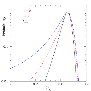
Figure 3: Probability distribution: $1-P_{\chi}[>\Delta\chi^{2},\nu=1]$ for $\Omega_{\Lambda}$ in the $r=20-21$ sample (short-dashed line), the LRG sample (long-dashed line) and the combined analysis (continuous middle curve). The range of $68\%$ and $95\%$ confidence regions in $\Omega_{\Lambda}$ are defined by the intersection with the corresponding horizontal lines.

Fig.4 shows the joint 2D contours for dark energy models with an effective equation of state $w=p/\rho$, assuming not perturbations in DE and a Hubble equation: $H^{2}/H_{0}^{2}=\Omega(1+z)^{3}+\Omega_{\Lambda}(1+z)^{3(1+w)}$. For each $(w,\Omega_{\Lambda})$ we derive $b\sigma_{8}$ consistently from the galaxy-galaxy auto-correlation data. We also marginalize over the uncertainties in $b\sigma_{8}$ and over $\sigma_{8}\in(0.65,0.85)$, to account for the WMAP3 $\sigma_{8}$ normalization for $w\neq-1$. The cosmological constant model $w=-1$, however, still remains a very good fit to the data. This is due to the large degeneracy of the equation of state parameter $w$ with $\Omega_{\Lambda}$. This degeneracy can be broken by supernovae SNIa data (eg see Corasaniti, Giannantonio and Melchiorri 2005 and Fig.8 in see Gaztañaga, Manera & Multamäki 2006).

4 Discussion

The objective of our analysis was primarily to check if we could confirm or refute with higher significance the findings of the WMAP1-SDSS1 cross-correlation by FGC03. With an increase in area of a factor of $\simeq 3.7$ in SDSS4, larger signal-to-noise and better understanding of foregrounds in WMAP3, our new analysis shows that the signal is robust. This is also in line with the first findings using optical (APM) galaxies by Fosalba & Gaztañaga (2004). The cross-correlation signal in WMAP3-SDSS4 seems slightly larger than in previous WMAP1-SDSS1 measurements which results in slightly larger values for $\Omega_{\Lambda}$ (see FGC03 and Gaztañaga, Manera & Multamäki 2006). This is probably due to sampling variance, as the SDSS4 volume has increase by almost a factor of 4 over SDSS1. We find little difference within the errors in the cross-correlation of WMAP1-SDSS4 and WMAP3-SDSS4 (see Fig.2).

The total S/N in Eq.4 of the WMAP3-SDSS4 correlation is $S/N\simeq 3.6$ for the $r=20-21$ sample and $S/N\simeq 3.0$ for the LRG, which gives a combined $S/N\simeq 4.7$, assuming the two samples are independent. We have checked the validity of this assumption by doing a proper join analysis where we include the covariance between the two samples. For the join analysis we find a $S/N\simeq 4.4$ with the first 2 dominant eigenvectors and $S/N\simeq 4.8$ with 4 eigenvectors.

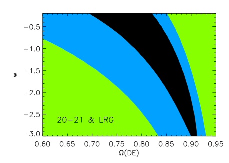
Figure 4: Two dimensional contours for $\Omega_{\Lambda}$ and $w$, the DE effective equation of state. The inner black contour limits the 1D marginalized $68\%$ confidence region ($\Delta\chi^{2}=1$). The other contour correspond to $95\%$ limits ($\Delta\chi^{2}=4$).

We find that a $\Lambda CDM$ model with $\Omega_{\Lambda}\simeq 0.83$ successfully explains the ISW effect for both samples of galaxies without need of any further modeling. The best fit for $\Omega_{\Lambda}$ for each individual sample are very close. This is significant and can be understood as a consistency test for the $\Lambda$CDM model.

The equation of state parameter appears to be very degenerate and it is not well constrained by current ISW data alone (see also Corasaniti, Giannantonio and Melchiorri 2005 and Gaztañaga, Manera & Multamäki 2006). Upcoming surveys such as the Dark Energy Survey (DES, www.darkenergysurvey.org), with deeper galaxy samples and more accurate redshift information should be able to break the $w-\Omega_{\Lambda}$ degeneracy and maybe shed new light on the the nature of dark energy.

References

- [Adelman-McCarthy et al ¡2006¿] Adelman-McCarthy, J. K., et al. 2006, ApJS, 162, 38
- [Afshordi et al ¡2004¿] Afshordi, N. , Loh, Y., Strauss, M.A., 2004, Phys. Rev D 69, 083524
- [Afshordi ¡2004¿] Afshordi,N., 2004, Phys. Rev D 70, 083536
- [Bennett et al ¡2003b¿] Bennett, C. L., et al. 2003b, ApJ.Suppl., 148, 97
- [Boughn & Crittenden ¡2004a¿] Boughn, S. P. & Crittenden, R. G.. 2004, Nature, 427, 45
- [Boughn & Crittenden ¡2004b¿] Boughn, S.P. & Crittenden, R. G., 2004, ApJ 612, 647-651
- [Brown et al ¡2003¿] Brown, M. L., et al. 2003, MNRAS, 341, 100
- [Corasaniti et al ¡2005¿] Corasaniti, P.S., Giannantonio, T., Melchiorri, A. 2005, Phys. Rev D 72, 023514
- [Crittenden & Turok¡1996¿] Crittenden, R. G., Turok, N., 1996, PRL, 76, 575
- [Dodelson et al.¡2002¿] Dodelson, S. et al. 2002, ApJ, 572, 140
- [Efstathiou ¡2003¿] Efstathiou, 2003, MNRAS, 346, L26
- [Eisenstein et al.¡2001¿] Eisenstein, D.J., et al, 2001, AJ, 122, 2267
- [Fosalba & Gaztañaga ¡2004¿] Fosalba, P., & Gaztañaga, E., 2004, MNRAS, 350, L37
- [Fosalba, Gaztañaga & Castander ¡2003¿] Fosalba P., Gaztañaga E., Castander F., 2003, ApJ, 597, L89
- [Fosalba et al. ¡2006¿] Fosalba, P. et al. 2006, in preparation
- [Gaztañaga et al ¡2003¿] Gaztañaga E., Wagg, J., Multamäki, T., Montaña, A., Hughes, D.H., 2003, MNRAS, 346, 47
- [Gaztañaga et al ¡2006¿] Gaztañaga E., Manera, M. & Multamäki, T., 2006, MNRAS, 365, 171
- [Górski et al ¡1998¿] Górski, K. M., Hivon, E., & Wandelt, B. D. 1999, in Proc. MPA-ESO Conf., Evolution of Large-Scale Structure: From Recombination to Garching, p.37, Ed. A.J.Banday, R.K.Seth, & L.A.N. da Costa (Enschede: PrintPartners Ipskamp)
- [Hinshaw et al ¡2003¿] Hinshaw, G. F. et al. 2003, ApJ.Suppl., 148, 63
- [Hinshaw et al ¡2006¿] Hinshaw et al. , 2006, astro-ph/0603451
- [Nolta et al ¡2004¿] Nolta M.R., et al., 2004, ApJ 608, 10
- [Oliveira-Costa et al ¡2004¿] Oliveira-Costa, A., Tegmark, M., Zaldarriaga, M., Hamilton, A., 2004, PRD, 69, 063516
- [Sachs & Wolfe¡1967¿] Sachs, R. K. & Wolfe, A. M. 1967, ApJ, 147, 73
- [Scranton et al ¡2003¿] Scranton et al. 2003, astro-ph/0307335.
- [Spergel et al ¡2006¿] Spergel et al. 2006, astro-ph/0603449
- [Tegmak et al ¡2003¿] Tegmark, M., Oliveira-Costa, A., Hamilton, A., 2003, PRD, 68, 123523